Methods and reagent-lot comparisons by regression analysis: Sample size considerations

Abstract

Background

Parametric regression analysis is widely used in methods comparisons and more recently in checking the concordance of test results following receipt of new reagent lots. The greater frequency of reagent-lot evaluations increases pressure to detect bias with smallest possible sample sizes (i.e. smallest consumption of time and resources). This study revisits bias detection using the joint slope, intercept confidence region as an alternative to slope and intercept confidence intervals.

Methods

Four cases were considered representing constant errors, proportional errors (constant CV) and two more complicated error patterns typical of immunoassays. Maximum:minimum range ratios varied from 2:1 to 2000:1. After setting a maximum tolerable difference a series of slope, intercept combinations, each of which predicted the critical difference, were systematically evaluated in simulations which determined the minimum sample size required to detect the difference, firstly using slope, intercept confidence intervals and secondly using the joint slope, intercept confidence region.

Results

At small to moderate range ratios, bias detection by joint confidence region required greatly reduced sample sizes to the extent that it should encourage reagent-lot evaluations or, alternatively, transform those already routinely performed into considerably less costly exercises.

Conclusions

While some software is available to calculate joint confidence regions in real-life analyses, shifting this testing method into the mainstream will require a greater number of software developers incorporating the necessary code into their regression programs. The computer program used to conduct this study is freely available and can be used to model any laboratory test.

Introduction

Parametric regression has long been employed in methods comparison studies. More recently a realisation that reagent-lot changes might be a significant source of errors^1–7 has directed increasing attention on formally evaluating new reagent lots before introducing them into routine use. Regression is an obvious candidate for conducting such evaluations. Methods comparisons are relatively rare (method changes typically occur years apart on average), but reagent-lot comparisons have a considerably greater frequency and the issue of detecting bias with the smallest possible sample size comes into sharper focus. This study compares the bias detection characteristics of slope and intercept confidence intervals (CIs) with the alternative of using the joint slope, intercept confidence region (CR). CRs are well established in statistical theory^8,9 but have been almost completely neglected for purposes of significance testing.

Figure 1 illustrates the relevant geometry using an example taken from Linnet’s well known treatise ¹⁰ on required sample size. He considered paired potassium results with concentration range 3–6 mmol/L. Method errors were assumed to be identical and constant with SD = 0.09 mmol/L. Using a uniform distribution of target values along the interval 3–6 mmol/L, 50 X, Y values were randomly drawn from Gaussian distributions with SD = 0.09 mmol/L. Slope and intercept were estimated by iteratively reweighted Deming regression, ¹¹ and the process was repeated 100 times. ¹² Figure 1(a) is a plot of the resulting 100 slope and intercept values. Intuition might suggest that the data points should have a roughly circular distribution about the true underlying values, indicated by the intersection of the dashed lines, but that is not the case in practice; slope and intercept are correlated and the smaller the maximum:minimum range ratio (2:1 in this case) the greater the correlation. Slope CIs are horizontal lines in the Figure 1(a) coordinate frame and they have the property that in repeated sampling experiments a certain fraction of them will enclose the true underlying slope. At the 5% significance level, for example, approximately 95% of CIs will enclose the true underlying slope and approximately 5% will not. Statistically significant proportional bias is detected when a data point and its slope CI are shifted sufficiently far left or right that the slope CI no longer encloses the true value. Similarly an intercept CI is a vertical line and statistically significant constant bias is detected when a data point and its intercept CI are shifted sufficiently far up or down that the CI no longer encloses the true value. 95% CIs for each of the 100 data points are shown in Figure 1(b) where the horizontal and vertical CI lines are plotted around each data point as a rectangle. Statistically significant bias is detected when a rectangle fails to enclose the intersection of the dashed lines. As expected, most rectangles in Figure 1(b) enclose the true values but a small fraction do not and collectively they represent three possible bias types; pure proportional bias (rectangle shifted left or right of the vertical dashed line but encloses the horizontal line), pure constant bias (rectangle shifted up or down from the horizontal dashed line but encloses the vertical line) and both (rectangle encloses no part of the dashed lines). Figure 1(c) shows the corresponding 95% CRs. Their elliptical shapes clearly indicate that they take full account of slope, intercept correlation. CIs do not. 95% CRs have the property that in sampling experiments of the type illustrated here approximately 95% will enclose the intersection of the dashed lines and approximately 5% will not. As with CI rectangles, statistically significant bias is detected when a CR fails to enclose the true values. CRs have the same potential as CIs for purposes of significance testing.

Figure 1.

(a) Plot of slope and intercept values obtained by Deming regression analysis of 100 simulated sets of N = 50 paired potassium results, with underlying relationship Y = X. (b) The data points and their associated 95% slope and intercept CIs (horizontal and vertical lines, respectively) plotted as CI rectangles. (c) The data points and their associated 95% joint slope, intercept CRs.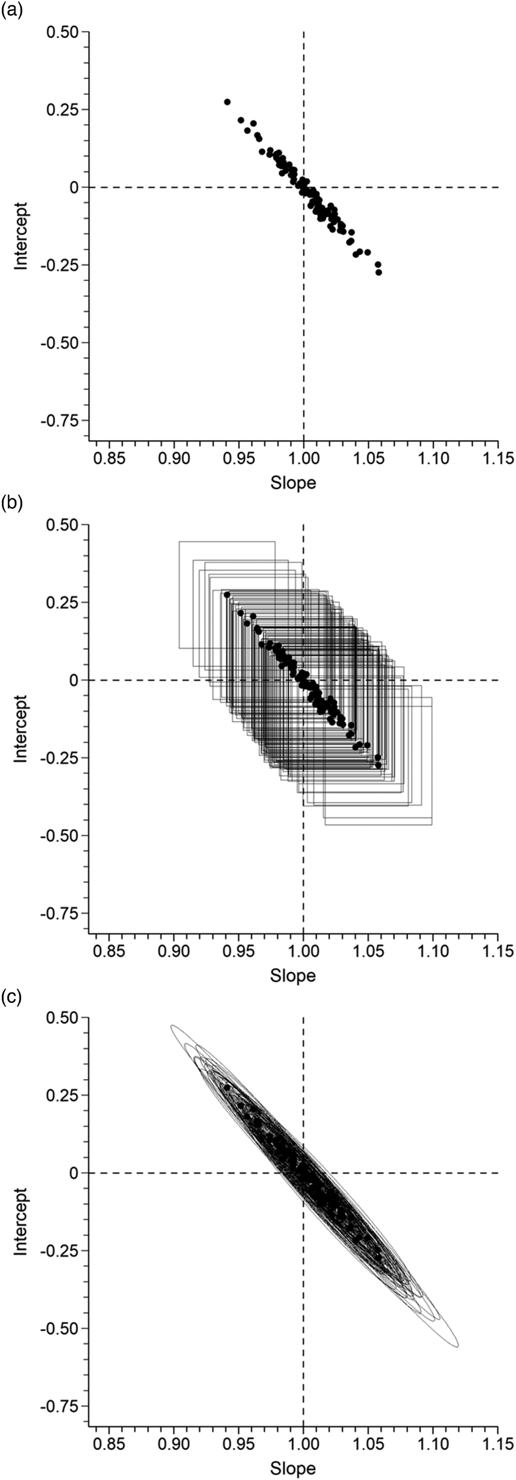

Bias occurs when underlying slope, intercept values are systematically shifted away from the intersection of the dashed lines in Figure 1. A very large shift implies that CI rectangles and CRs will easily detect the bias by failing to enclose the intersection of the dashed lines. Small shifts might not be reliably detected. Increasing the number of X, Y pairs (sample size) reduces the sizes of CI rectangles and CRs thereby improving the probability of detecting bias. The essential questions are, (1) what degree of bias do we consider sufficiently serious that we would want to reliably detect it, if it was present? (2) what sample size do we need for reliable detection? Figure 1 raises an additional question; what method of testing should be used? The geometry clearly suggests that, for a given sample size, CRs will detect smaller left-right shifts (pure proportional bias), smaller up-down shifts (pure constant bias) and smaller diagonal shifts, unless the shift just happens to lie roughly along the 45° diagonal delineated by the data points. Putting that another way; comparable detection success using CI rectangles would require some shrinkage, that is, a larger sample size.

This study uses simulations to put numbers on required sample sizes. Linnet ¹⁰ provided a pair of detailed worked examples representing constant and proportional error patterns. These are re-evaluated together with two hypothetical sets of immunoassay data.

Methods

In the four cases considered here, X and Y errors were assumed to be identical (as might be expected in a reagent-lot comparison), although it is a simple matter to incorporate unequal errors into simulations if necessary. In each case, a uniform distribution of target values was used and randomly drawn sets of paired X, Y values were analysed by iteratively reweighted Deming regression using X, Y values or adjusted X, Y values to update the weights, as per York. ¹³ Assigned weights were the reciprocal of predicted variance at each X, Y or adjusted X, Y value.

Required sample sizes were determined for various combinations of slope and intercept values (described below) by repeatedly drawing 10,000 sets of X, Y pairs, of differing sample size, examining CI rectangle and CR enclosure rates and iterating toward the sample size corresponding to a 90% detection rate using a bisection approach. ¹²

Potassium

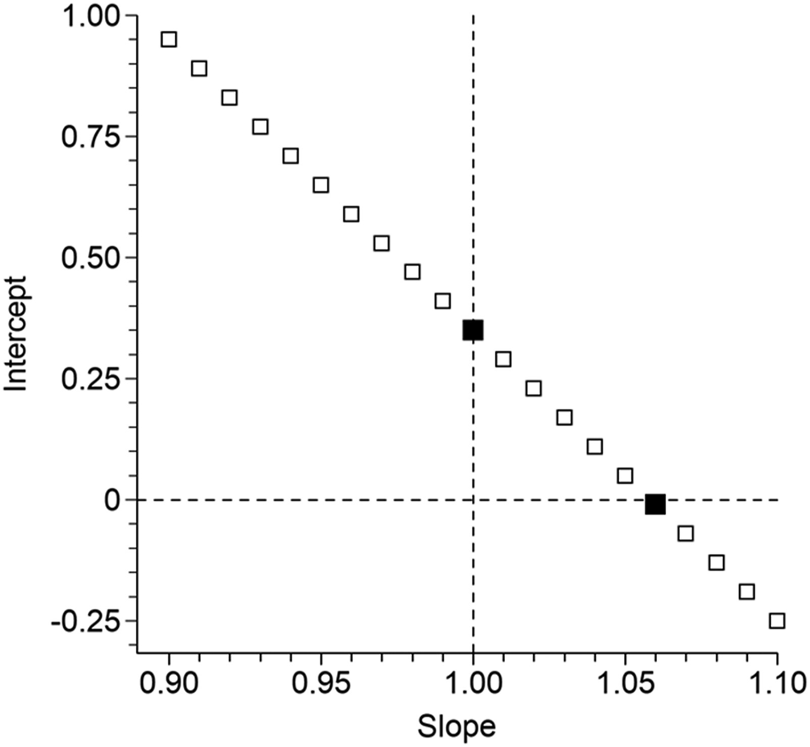
Assumed range 3–6 mmol/L (range ratio 2:1), and constant SD = 0.09 mmol/L (i.e. weights were the reciprocal of variance (σ²) = 0.0081). Using CLIA 88 guidelines, Linnet determined the maximum allowable difference between methods to be 0.35 mmol/L at the upper end of the range. Treating slope and intercept as independent quantities, the two combinations requiring reliable detection are therefore [slope = 1, intercept = 0.35] and [slope = (6 + 0.35)/6 = 1.0583, intercept = 0]. For convenience, Linnet adjusted the second combination to [slope = 1.06, intercept = 0]. These combinations equate to a difference of exactly or close to 0.35 mmol/L at the upper end of the range. Linnet derived equations to calculate the minimum sample sizes required to give a 90% probability of detecting these critical slope and intercept values, at the 5% significance level. There are, however, an infinite number of slope, intercept combinations that equate to a difference of 0.35 mmol/L at the upper end of the range and simulations are a convenient way to investigate a subset of them. Slope values in the range 0.9 to 1.1, in increments of 0.01, were paired with intercept values given by the formula

$\text{Intercept}=6.35\hspace{0.17em}–\hspace{0.17em}6\text{xSlope},$

to produce 21 combinations, all of which predict values very close to the 0.35 mmol/L difference, we wish to detect at the upper end of the range.

Glucose

Assumed range 600–3000 mg/L (range ratio 5:1), and proportional errors (constant CV = 3%). Regression weights were therefore assigned as the reciprocal of σ² = 0.0009U² where U denotes an X or Y value, or an adjusted X or Y value. Using CLIA 88 guidelines, Linnet determined the maximum allowable difference between methods to be 63 mg/L at concentration 1260 mg/L which was taken as a fasting plasma glucose limit for diabetes. The two combinations requiring reliable detection are therefore [slope = 1, intercept = 63] and [slope = (1260 + 63)/1260 = 1.05, intercept = 0]. Evaluation combinations were obtained by pairing the 21 slope values described in the previous section with intercept values given by

$\text{Intercept}=1323\hspace{0.17em}–\hspace{0.17em}1260\text{xSlope}.$

Total triiodothyronine (T3)

Based on an in-house radioimmunoassay (reference range: 1.2–2.8 nmol/L). Assumed range 0.5–8 nmol/L (range ratio 16:1). Regression weights were assigned as the reciprocal of variances predicted by the variance function, σ² = β₁ + β₂U^J, estimated from internal QC data, ¹⁴ with parameter values β₁ = 0.00603, β₂ = 0.000263 and J = 3.355. The maximum allowable difference was arbitrarily set at 5% at the upper limit of the reference range (=0.14 nmol/L). Following Linnet’s proposal the two combinations requiring reliable detection are therefore [slope = 1, intercept = 0.14] and [slope = 1.05, intercept = 0]. Evaluation combinations were obtained by pairing the 21 slope values described above with intercept values given by

$\text{Intercept}=2.94\hspace{0.17em}–\hspace{0.17em}2.8\text{xSlope}.$

Thyrotropin (TSH)

Based on an immunoluminometric assay (‘Access’ instrument, Beckman Coulter, Fullerton, CA, USA), reference range: 0.25–2.5 mU/L. Assumed range 0.015–30 mU/L (range ratio 2000:1). Regression weights were assigned as the reciprocal of variances predicted by the variance function, σ² = (β₁ + β₂U)^J, estimated from method evaluation data, ¹⁴ with parameter values β₁ = 0.008936, β₂ = 0.044 and J = 2.4718. The maximum allowable difference was arbitrarily set at 5% at the lower limit of the reference range (=0.0125 mU/L). The two combinations requiring reliable detection are therefore [slope = 1, intercept = 0.0125] and [slope = 1.05, intercept = 0]. Evaluation combinations were obtained by pairing the 21 slope values described above with intercept values given by

$\text{Intercept}=0.2625\hspace{0.17em}–\hspace{0.17em}0.25\text{xSlope}.$

Results

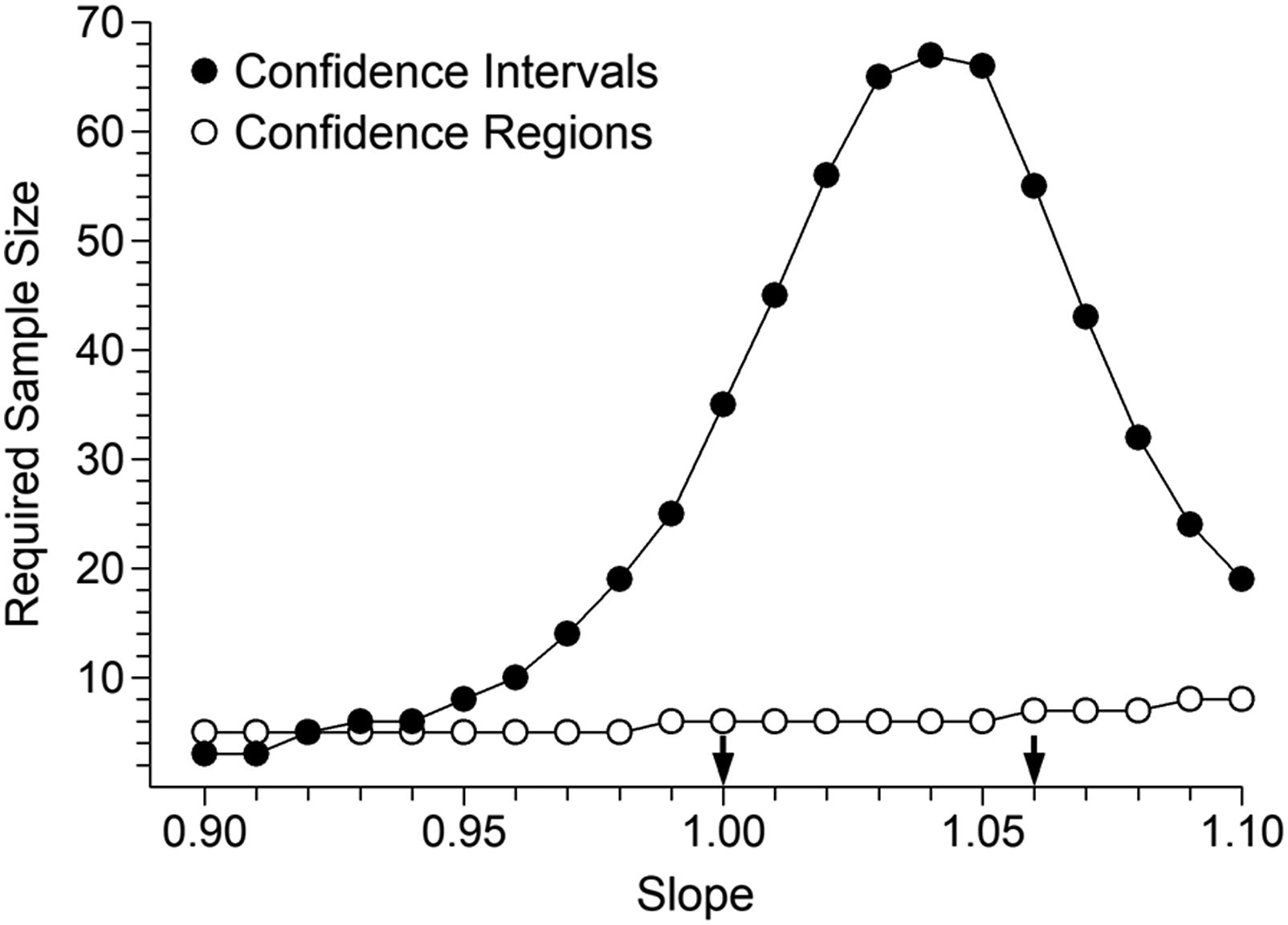
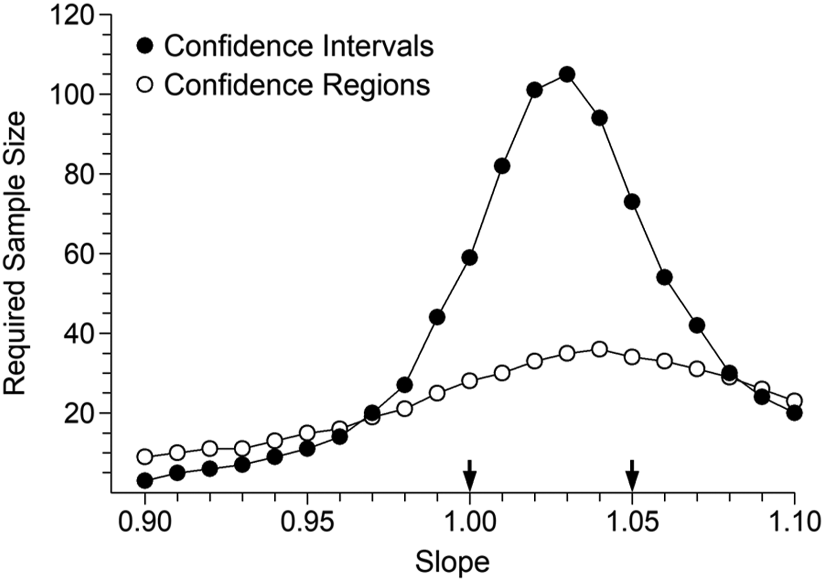
Figure 2 is a plot of the 21 combinations of slope and intercept values used for the potassium example (similar plots could be easily constructed for the other cases). The two solid data points indicate the combinations proposed by Linnet. Each data point predicts the difference we seek to detect but their locations have widely differing distances from the intersection of the dashed lines. In principle, the shorter the distance from the intersection of the dashed lines, the greater the required sample size, and vice versa. It is worth noting that the data points lying closest to the intersection are those located between Linnet’s evaluation combinations. Figure 3 illustrates sample sizes required to guarantee 90% bias detection, at the 5% significance level. Arrows mark the evaluation combinations proposed by Linnet. The required sample size by CR testing appears to be slowly rising but extending the simulations out to Slope = 1.20 produced a mixture of N = 8 and N = 9 as required sizes. The N = 8 value, observed at [slope = 1.10, intercept = −0.25], could be taken as a reasonable estimate. Some might be sceptical that CR testing requires a sample size no greater than N = 8. The geometry, along the lines of Figure 1(c), is shown in a Supplemental file.

Figure 2.

Potassium evaluation. Combinations of slope and intercept values that equate to a value of approximately 6.35 mmol/L at concentration 6 mmol/L, that is, positive bias of approximately 0.35 mmol/L. The solid data points indicate the combinations where bias can be attributed to either pure constant bias or approximately pure proportional bias.

Figure 3.

Potassium evaluation. Sample sizes required to achieve 90% detection of positive bias of 0.35 mmol/L at concentration 6 mmol/L, at the 5% significance level. The 21 evaluation slope and intercept combinations are illustrated in Figure 2. The arrows indicate the two combinations which represent either pure constant bias (left) or approximately pure proportional bias (right), that is, the combinations evaluated by Linnet. ¹⁰

Figures 4 and 5 show corresponding results for glucose and T3, respectively. The increase in range ratio from 2:1 (potassium) to 5:1 (glucose) and 16:1 (T3) manifests as reduced parameter correlation and therefore a decrease in the relative advantage of CRs versus CIs (although the differences remain substantial in practical terms).

Figure 4.

Glucose evaluation. Sample sizes required to achieve 90% detection of positive bias of 63 mg/L at concentration 1260 mg/L, at the 5% significance level. The arrows indicate the two combinations which represent either pure constant bias (left) or pure proportional bias (right), that is, the combinations evaluated by Linnet. ¹⁰

Figure 5.

Total T3 evaluation. Sample sizes required to achieve 90% detection of positive bias of 0.14 nmol/L at concentration 2.8 nmol/L, at the 5% significance level. The arrows indicate the two combinations which represent either pure constant bias (left) or pure proportional bias (right).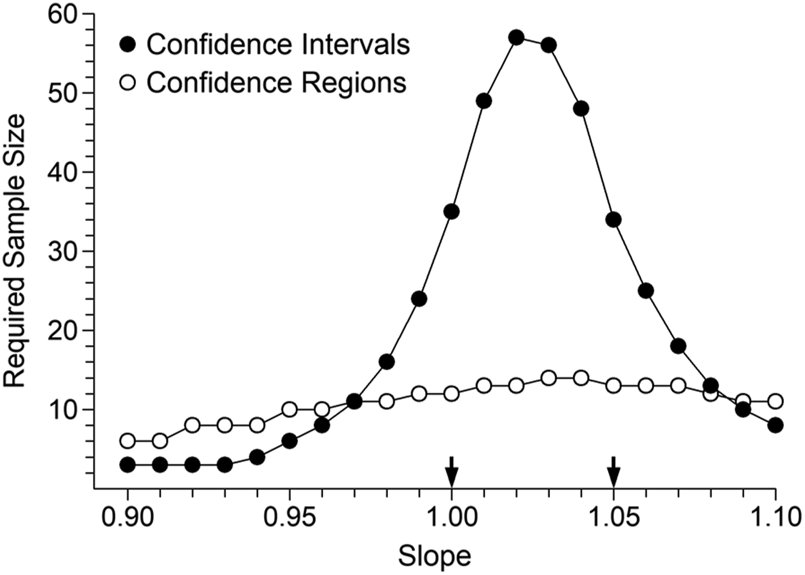

Results in Figures 3–5 were obtained using a uniform distribution of target values. Additional simulations using a roughly Gaussian distribution of target values resulted in required sample size increases of 55%, 35% and 40% for CIs relative to those shown in Figures 3–5, respectively. Results for CRs could not be distinguished from those illustrated. The message is clear; those who persist with CIs should avoid a high density of specimens in the central part of the range. A right skewed distribution is often seen in clinical settings, and additional simulations using that pattern of target values showed no obvious differences to the potassium and glucose results shown in Figures 3 and 4. In the T3 case, reductions in required CI and CR sample sizes were seen over the left side of the range in Figure 5, but no reduction at the peak sample size values.

The TSH results illustrated in Figure 6 show a markedly different pattern and a large sample size requirement regardless of testing method. This is an example of how not to conduct a comparison. A uniform target distribution was used when the aim was to detect a difference located within the lowest 1% of the range. As might be expected, a right skewed distribution of target values greatly reduced required sample sizes, with further improvement available via a range reduction. This is illustrated in the Supplemental file.

Figure 6.

TSH evaluation. Sample sizes required to achieve 90% detection of positive bias of 0.0125 mU/L at concentration 0.25 mU/L, at the 5% significance level. The arrows indicate the two combinations which represent either pure constant bias (left) or pure proportional bias (right).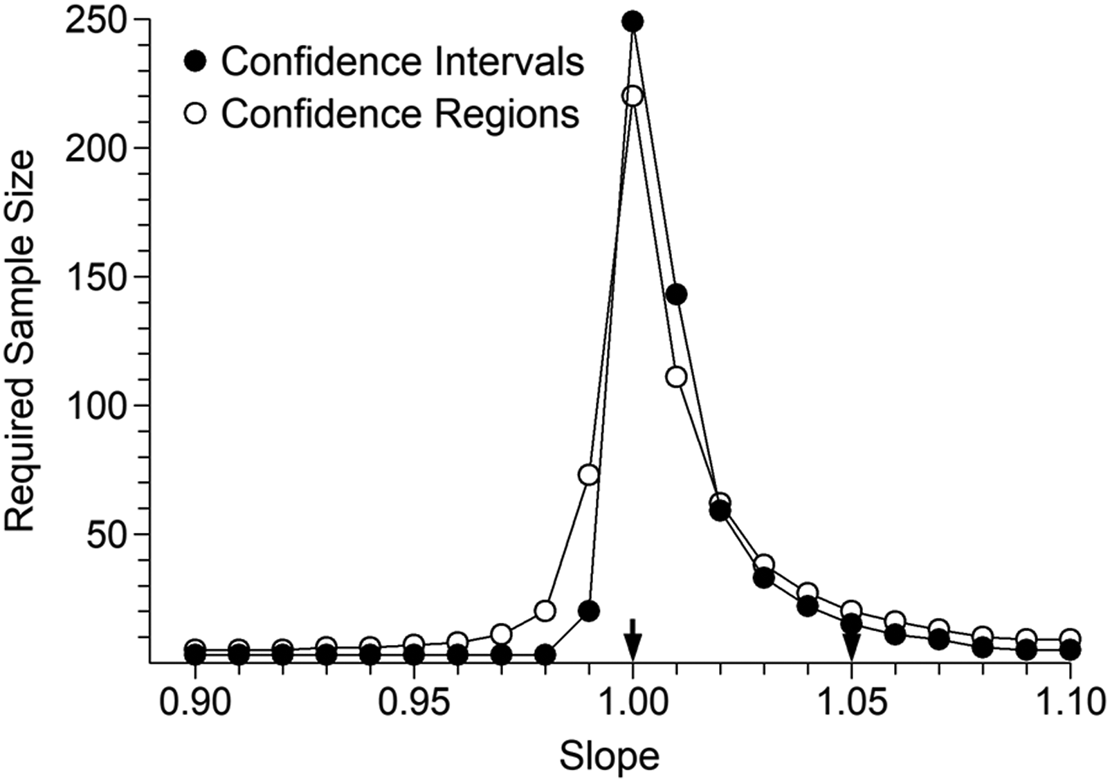

Results in Figures 3–6 evaluated positive differences from the line of identity. Evaluating the corresponding negative differences would involve slope, intercept combinations parallel to those in Figure 2 (or their equivalents for the other cases considered) but shifted vertically down to an equal distance below the intersection of the dashed lines. Results should appear as a mirror image of those currently plotted in Figures 3–6, that is, the tick mark values remain the same but each data set is rotated 180°. Small discordances might be seen in practice because simulated Y values would be systematically smaller and therefore have slightly different assigned weights (constant error cases excepted).

The slope, intercept combinations toward the left extreme of Figure 2 occupy locations that lie increasingly close to the 45° diagonal passing through the intersection of the dashed lines. CRs offer no advantage along that particular alignment and could be predicted to require larger sample sizes (consider distances across CI rectangles and CRs in Figure 1, viewed along the 45° diagonal formed by the data points). The expected effect was observed in all sets of simulation results, being particularly pronounced in Figure 4, but those combinations are irrelevant in the context of determining required sample sizes.

Discussion

Linnet ¹⁰ gave clear guidelines for determining a maximum tolerable difference which he translated into maximum allowable deviations of slope and intercept from 1 and 0, respectively. Unfortunately, his sample size equations treated slope and intercept as independent quantities and did not provide for variable combinations of the two. Simulations provide an alternative and robust way of experimenting. It is a simple matter to specify real-life error characteristics thereby providing not only for unequal X and Y errors (likely to be relevant for methods comparisons) but also for those medical laboratory tests that do not conform to simple constant or proportional error patterns. Two points are worth noting. Firstly, in many cases, sample size determination would require just a few evaluations between the slope, intercept combinations proposed by Linnet. If a peak is observed (e.g. Figures 4 and 5) that would conclude the exercise. Secondly, sample size determination in the reagent-lot context should only need to be done once for any particular test, and revisited only if there is an appreciable shift in test uncertainty.

Every data set used in Figures 3–6 represented systematic bias, calculated to be the maximum we are prepared to tolerate. The objective is the least costly way of being reliably alerted if that degree of bias (or larger) actually exists. CIs are currently the mainstream alert mechanism but simulation results confirm the markedly greater statistical power associated with CRs, at least with small to moderate range ratios. The underlying theory of slope, intercept correlation and joint parameter CRs has been extensively described over many decades, for example, Refs. 8,9. As long ago as 1979, Munson and Rodbard ¹⁵ suggested the use of CRs in an immunoassay context. Statistical power considerations and numerical details have been previously reported. ¹⁶ The obvious question is: why are CRs not used routinely?

Some analysts might be unaware of alternatives to CIs, but the main reason is almost certainly a lack of software. Castillo and Cahya ¹⁷ described a confidence region program coded using the algebra package MAPLE. Pallmann ¹⁸ developed a program written in R-code. Variance Function Program ¹⁴ computes and plots CRs and is specifically aimed at medical laboratory data. However, a tiny handful of programs are not sufficient. Progress will require more developers of regression software, whether standalone programs or those embedded within general statistics packages, to firstly recognise the practical advantages of CRs and secondly to develop the necessary code. Determining whether a CR encloses a particular point, for example, the intersection of the dashed lines in Figure 1, is no more complicated than computing CIs. It is arguably simpler in the case of Deming regression. Calculation of CR plotting coordinates entails nothing more complicated than solving quadratic equations. ¹⁶ In short, the calculations are far removed from the ‘insurmountably difficult’ category. In a medical laboratory context, there is scope for considerable savings in time and resources and especially when evaluations might be required relatively frequently, as is the case with reagent-lot changes.

Finally, the Windows computer program ¹² used to produce the graphs in Figure 1 and the data points plotted in Figures 3–6 is freely available. It can be used to investigate any combination of range ratio, error patterns, data distribution, and user defined power and significance levels. It generates randomly drawn X, Y pairs according to user specifications, but also allows the importing and evaluation of data created by an external simulation process.

Supplemental Material

Supplemental Material - Methods and reagent-lot comparisons by regression analysis: Sample size considerations

Supplemental Material for Methods and reagent-lot comparisons by regression analysis: Sample size considerations by William A Sadler in Annals of Clinical Biochemistry