Sage Journals: Discover world-class research

Abstract

A kinetic modeling approach for the quantification of in vivo tracer studies with dynamic positron emission tomography (PET) is presented. The approach is based on a general compartmental description of the tracer's fate in vivo and determines a parsimonious model consistent with the measured data. The technique involves the determination of a sparse selection of kinetic basis functions from an overcomplete dictionary using the method of basis pursuit denoising. This enables the characterization of the systems impulse response function from which values of the systems macro parameters can be estimated. These parameter estimates can be obtained from a region of interest analysis or as parametric images from a voxel-based analysis. In addition, model order estimates are returned that correspond to the number of compartments in the estimated compartmental model. Validation studies evaluate the methods performance against two preexisting data led techniques, namely, graphical analysis and spectral analysis. Application of this technique to measured PET data is demonstrated using [¹¹C]diprenorphine (opiate receptor) and [¹¹C]WAY-100635 (5-HT1A receptor). Although the method is presented in the context of PET neuroreceptor binding studies, it has general applicability to the quantification of PET/SPECT radiotracer studies in neurology, oncology, and cardiology.

Keywords

PET Tracer kinetics Compartmental modeling Parameter estimation Basis pursuit de-***noising Sparse basis selection

The development of positron emission tomography (PET) over the last 2 decades has provided neuroscientists with a unique tool for investigating the neurochemistry of the human brain in vivo. The ever-increasing library of radiolabeled tracers allows for imaging of a range of biochemical, physiologic and pharmacological processes. Each radiotracer has its own distinct behavior in vivo, and their characterization is an essential component for the development of new imaging techniques and their translation into clinical applications. Estimation of quantitative biologic images from the rich four-dimensional (4D) spatiotemporal data sets requires the application of appropriate tomographic reconstruction and tracer kinetic modeling techniques. The latter are used to estimate biologic parameters by fitting a mathematical model to the time–activity curve (TAC) of a region of interest or voxel. Calculations at the voxel level produce parametric images but are associated with an increase in noise for the TACs. Analysis strategies must therefore be robust to noise, yet fast enough to be practical.

There is a range of quantitative PET tracer kinetic modeling techniques that return biologically based parameter estimates. These techniques may be broadly divided into model-driven methods (Kety, 1951; Sokoloff et al., 1977; Phelps et al., 1979; Mintun et al., 1984; Huang and Phelps, 1986; Gunn et al., 2001) and data-driven methods (Gjedde, 1982; Patlak et al., 1983; Patlak and Blasberg, 1985; Logan et al., 1990; Logan et al., 1996; Cunningham and Jones, 1993). The clear distinction is that the data-driven methods require no a priori decision about the most appropriate model structure. Instead, this information is obtained directly from the kinetic data.

Model-driven methods use a particular compartmental structure to describe the behavior of the tracer and allow for an estimation of either micro or macro system parameters. Well-established compartmental models in PET (Fig. 1) include those used for the quantification of blood flow (Kety, 1951), cerebral metabolic rate for glucose (Sokoloff et al., 1977), and for neuroreceptor ligand binding (Mintun et al., 1984). Further developments have produced a series of reference tissue models that avoid the need for blood sampling (Blomqvist et al., 1989; Cunningham et al., 1991; Hume et al., 1992; Lammertsma et al., 1996; Lammertsma and Hume, 1996; Watabe et al., 2000). Parameter estimates are obtained from a priori specified compartmental structures using one of a variety of least-squares fitting procedures: linear least squares (Carson, 1986), nonlinear least squares (Carson, 1986), generalized linear least squares (Feng et al., 1996), weighted integration (Carson et al., 1986), or basis function techniques (Koeppe et al., 1985; Cunningham and Jones, 1993; Gunn et al., 1997).

FIG. 1.

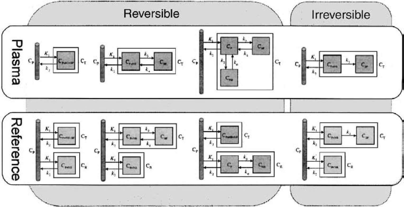
A range of positron emission tomography (PET) compartmental models commonly used to quantify PET radiotracers. These include models for tracers that exhibit reversible and irreversible kinetics and models that use either a plasma or reference tissue input function.

Data-driven methods such as graphical analysis (Gjedde, 1982; Patlak et al., 1983; Patlak and Blasberg, 1985; Logan et al., 1990; Logan et al., 1996) or spectral analysis (Cunningham and Jones, 1993) derive macro system parameters from a less constrained description of the kinetic processes. The graphical methods (Patlak and Logan plots) use a transformation of the data such that a linear regression of the transformed data yields the macro system parameter of interest and are attractive and elegant owing to their simplicity. However, they require the determination of when the plot becomes linear, they may be biased by statistical noise (Slifstein and Laruelle, 2000), and they fail to return any information about the underlying compartmental structure. Appendix A gives a formal derivation of the Logan plot and shows that it is valid for an arbitrary number of compartments for both plasma and reference tissue input models when the data are free from noise. Spectral analysis (Cunningham and Jones, 1993) characterizes the systems impulse response function (IRF) as a positive sum of exponentials and uses nonnegative least squares to fit a set of these basis functions to the data. The macro system parameters of interest are then calculated as functions of the IRF (Cunningham and Jones, 1993; Gunn et al., 2001). Spectral analysis also returns information on the number of tissue compartments evident in the data and is defined as a transparent technique. Schmidt (1999) showed that for the majority of plasma input models, the observation of all compartments led to only positive coefficients, and as such the spectral analysis (Cunningham and Jones, 1993) solution using nonnegative least squares is valid. It is straightforward, however, to deduce that for reference tissue input models, negative coefficients can be encountered and that this approach is strictly not valid [see Appendix C in Gunn et al. (2001)].

Recently, we have published general theory for both plasma input and reference tissue input models (Gunn et al., 2001). This work shows that a general PET tracer compartmental system may be characterized in terms of its IRF, and that this is independent of the administration of the tracer and is therefore applicable to both bolus and bolus-infusion methodologies. The term tracer excludes multiple injection protocols involving low specific activity injections that are classed as nontracer studies and lead to nonlinear compartmental systems. In brief, a general PET tracer compartmental model leads to a set of first-order linear differential equations. This set of equations may be solved to yield an expression for the total tissue radioactivity concentration in terms of either a plasma input function or a suitable reference tissue input function. These results are derived from linear systems theory, which leads to the deduction that the IRF comprises solely exponentials and a delta function (Gunn et al., 2001). This work forms the foundation for the presented method: data-driven estimation of parametric images based on compartmental theory (DEPICT).

DEPICT allows for the estimation of parametric images or regional parameter values from dynamic PET data. DEPICT requires no a priori description of the tracers fate in vivo; it derives the model description from the data and it returns the number of compartments (model order). This transparent modeling technique has application to a wide range of PET radiotracers, but the emphasis here is with respect to the analysis of radioligands that bind to specific neuroreceptor sites.

THEORY

This section introduces the theory behind DEPICT. First, the general forms for plasma input and reference tissue input models are presented; second, key parameters for neuroreceptor binding studies are cast in this framework; and third, the general parameter estimation approach is constructed using basis functions and solved via basis pursuit denoising. The method encompasses the majority of linear compartmental systems, which are applicable to tracer studies with an arbitrary input function. It assumes that there is only one form (the parent compound) in which radioactivity enters the tissue from the arterial plasma. Specifically, those models that are defined by definitions 1 and 2 in Gunn et al. (2001) are considered. These sets of models encompass all noncyclic systems, the subset of cyclic systems in which the product of rate constants is the same regardless of direction for every cycle and requires the eigenvalues of the system to be distinct.

Plasma input models

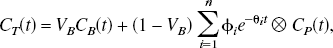
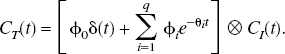
The general equation for a plasma input compartmental model is given by

C_{T} (t) = V_{B} C_{B} (t) + (1 - V_{B}) \sum_{i = 1}^{n} ϕ_{i} e^{- θ_{i} t} \otimes C_{P} (t),

(1)

where n is the total number of tissue compartments in the target tissue, ⊗ is the convolution operator, V_B is the fractional blood volume, C_T,C_P, and C_B are the concentration time courses in the target tissue, plasma, and whole blood, respectively. The delivery of the tracer to the tissue is given by

K_{1} = \sum_{i = 1}^{n} ϕ_{1}

Reversible kinetics [θ_i > 0]. For compartmental models that exhibit reversible kinetics, the volume of distribution, V_D, which is equal to the integral of the impulse response function, is given by

V_{D} = \sum_{i = 1}^{n} \frac{ϕ_{i}}{θ_{i}} .

(2)

Irreversible kinetics [θ_i≠n >0, θ_n = 0]. For compartmental models that exhibit irreversible kinetics, the net irreversible uptake rate constant from plasma, K_I, is given by

K_{I} = ϕ_{n} .

(3)

Reference tissue input models

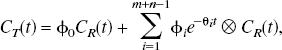
The general equation for a reference tissue input compartmental model is given by

C_{T} (t) = ϕ_{0} C_{R} (t) + \sum_{i = 1}^{m + n - 1} ϕ_{i} e^{- θ_{i} t} \otimes C_{R} (t),

(4)

where m is the total number of tissue compartments in the reference tissue, and n is the total number of tissue compartments in the target tissue, C_T and C_R are the concentration time courses in the target and reference tissues, respectively, and R_I (= φ₀) is the ratio of delivery of the tracer between the target and reference tissue. This definition excludes the presence of blood volume components to either of the tissues. Explicit formulation including a blood volume term has been given previously (Gunn et al., 2001).

Reversible target tissue kinetics [θ_i > 0]. For reference tissue models that exhibit reversible kinetics in both the target and reference tissues, the volume of distribution ratio is given by the integral of the impulse response of the system,

\frac{V_{D}}{V_{D}^{'}} = ϕ_{0} + \sum_{i = 1}^{m + n - 1} \frac{ϕ_{i}}{θ_{i}} .

(5)

Irreversible target tissue kinetics [θ_i≠m+n-1 >0, θ_{m+n- 1} = 0]. For reference tissue models that exhibit irreversible kinetics in the target tissue and reversible kinetics in the reference tissue, the normalized irreversible uptake rate constant from plasma is given by

\frac{K_{I}}{V_{D}^{'}} = ϕ_{m + n - 1} .

(6)

Parameters for neuroreceptor binding studies

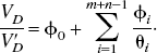
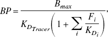
For reversible neuroreceptor binding studies, the binding potential may be calculated from the macro parameters, using either a plasma or reference tissue input function, under the assumption that the volume of distribution of the free and nonspecific binding is the same in the target and reference tissues. Throughout this article, the term “binding potential” is used interchangeably to refer to BP [the binding potential as originally defined by Mintun et al. (1984)], BP.f₂ and BP.f₁ where f₂ and f₁ are the tissue and plasma free fractions respectively. For a reference tissue input analysis, BP.f₂ is the only binding potential estimate possible, whereas with a plasma input analysis it is possible to obtain estimates for BP.f₁, BP.f₂, and if a separate measure of the plasma free fraction exists, BP. The binding potential is a useful measure of receptor specific parameters, which includes both the maximum concentration of receptor sites and the affinity,

B P = \frac{B_{m a x}}{K_{D_{T r a c e r}} (1 + \sum_{i} \frac{F_{i}}{K_{D_{i}}})},

(7)

where B_max is the maximum concentration of receptor sites, K_DTracer is the equilibrium disassociation rate constant of the radioligand, and F_i and K_Di are the free concentration and equilibrium disassociation constants of i competing ligands. To derive values for both the receptor concentration and affinity, it is necessary to perform a multiinjection study with differing specific activities of the radioligand. A summary of commonly used receptor binding parameters and their calculation from the general form of the IRF are given in Table 1. For further details see Gunn et al. (2001). The relative merits of these different binding parameters are discussed elsewhere (Laruelle, 2000).

TABLE 1.

Calculation of commonly used binding parameters from the general impulse response function

Parameter	Target	Reference	Input	Calculation
V_D	R	—	C_P	$\sum_{i = 1}^{n} \frac{ϕ_{i}}{θ_{i}}$
K_I	I	—	C_P	φ_n
BP.f₁	R	R	C_P	$\sum_{i = 1}^{n} \frac{ϕ_{i}}{θ_{i}} - \sum_{i = 1}^{m} \frac{ϕ_{i}}{ϑ_{i}}$
BP.f₂	R	R	C_P	$\frac{\sum_{i = 1}^{n} \frac{ϕ_{i}}{θ_{i}}}{\sum_{i = 1}^{m} \frac{ϕ_{i}}{ϑ_{i}}} - 1$
BP.f₂	R	R	C_R	$ϕ_{0} - 1 + \sum_{i = 1}^{m + n - 1} \frac{ϕ_{i}}{θ_{i}}$
$\frac{K_{I}}{V_{D}^{'}}$	I	R	C_R	φ_m+n-1

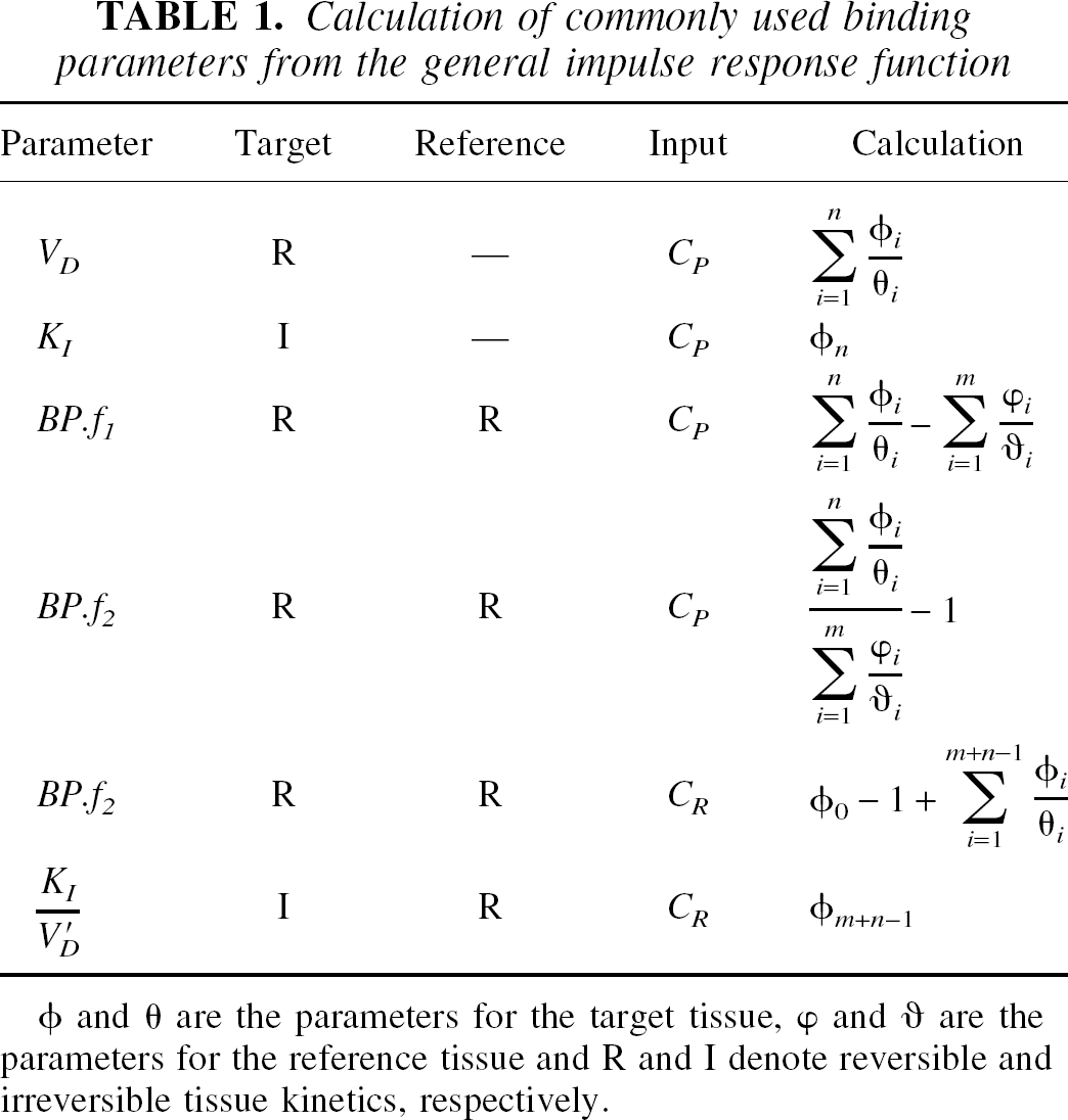
φ and θ are the parameters for the target tissue, φ and υ are the parameters for the reference tissue and R and I denote reversible and irreversible tissue kinetics, respectively.

Construction of the general model in a basis function framework

Plasma input¹ and reference tissue input PET compartmental models are characterized by

C_{T} (t) = [ϕ_{0} δ (t) + \sum_{i = 1}^{q} ϕ_{i} e^{- θ_{i} t}] \otimes C_{I} (t) .

(8)

where C_T is the tissue concentration time course and C_I is the concentration time course of the input function (plasma or reference tissue). This can be expressed as an expansion on a basis

C_{T} (t) = \sum_{i = 0}^{N} ϕ_{i} ψ_{i} (t),

(9)

where

ψ_{0} (t) = C_{I} (t),

(10)

ψ_{i} (t) = \int_{0}^{t} e^{- θ_{i} (t - τ)} C_{I} (τ) d τ .

(11)

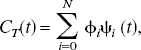
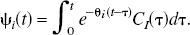
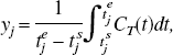
A set of N values for θ_i may be prechosen from a physiologically plausible range θ_min ⩽ θ_i ⩽ θ_max. Here, the θ_i values are spaced in a logarithmic manner to elicit a suitable coverage of the kinetic spectrum. Other possibilities for the spacing of the basis exist such as an equiangular scheme (Cunningham et al., 1998). For data that have not been corrected for the decay of the isotope, θ_min may be chosen as (or close to the decay constant (θ_min = λ min⁻¹) for the radioisotope and θ_max may be chosen as a suitably large value (θ_max = 6 min⁻¹). For reversible systems, where the calculation of V_D or BP.f₂ is the goal, the choice of a value for θ_min, which is slightly bigger than λ, can suppress the calculation of infinite V_D and BP.f₂ values from noisy data. PET measurements are acquired as a sequence of (F) temporal frames. Thus, the continuous functions must be integrated over the individual frames and normalized to the frame length to correspond to the data sampling procedure. The tissue observations, y, already exist in this form and correspond to

y = {[y_{1} … y_{F}]}^{T},

(12)

y_{j} = \frac{1}{t_{j}^{e} - t_{j}^{s}} \int_{t_{j}^{s}}^{t_{j}^{e}} C_{T} (t) d t,

and the matrix of kinetic basis functions (or dictionary), are precalculated as

\begin{array}{l} ψ = [\begin{array}{l} ψ_{01} & ψ_{11} & \dots & ψ_{N 1} \\ ⋮ & ⋮ & ⋮ & ⋮ \\ ψ_{0 F} & ψ_{0 F} & \dots & ψ_{N F} \end{array}], \\ ψ_{0 j} = \frac{1}{t_{j}^{e} - t_{j}^{s}} \int_{t_{j}^{s}}^{t_{j}^{e}} C_{I} (t) d t, \\ ψ_{i j} = \frac{1}{t_{j}^{e} - t_{j}^{s}} \int_{t_{j}^{s}}^{t_{j}^{e}} \int_{0}^{t} e^{- θ_{i} (t - τ)} C_{I} (τ) d t, \end{array}

(13)

ψ_{0 j} = \frac{1}{t_{j}^{e} - t_{j}^{s}} \int_{t_{j}^{s}}^{t_{j}^{e}} C_{I} (t) d t,

ψ_{i j} = \frac{1}{t_{j}^{e} - t_{j}^{s}} \int_{t_{j}^{s}}^{t_{j}^{e}} \int_{0}^{t} e^{- θ_{i} (t - τ)} C_{I} (τ) d t,

where t^s_j and t^e_j are the sequences of start and end frame times (j = 1, …, F). For all practical purposes (i.e., choosing a large enough value for N to obtain a good coverage of the kinetic spectrum), this leads to an overcomplete basis (N > F – 1), which by definition is nonorthogonal. Examples bases for a plasma and reference tissue input are displayed in Fig. 2. To determine the fit to the data, it is necessary to solve the underdetermined system of equations,

y ≅ Ψ ϕ .

(14)

To account for the temporally varying statistical uncertainty of the measurements, it is more appropriate to consider the weighted least-squares problem,

W^{\frac{1}{2}} y ≅ W^{\frac{1}{2}} Ψ ϕ,

(15)

where W is the inverse of the covariance matrix. Given the statistical independence of the frames, W is diagonal. These diagonal elements can be approximated from the total image TAC and frame durations (Mazoyer et al., 1986). The weighted least-squares solution is simply obtained by weighting both the data and the basis functions, i.e., y is replaced by W^1/2y and Ψ is replaced by W^1/2Ψ. On solution of this equation, the appropriate macro parameters (V_D, K_I, K₁, V_D/V′_D, K_I/K′_D, R_I) may be calculated from the φs (see Eqs. 2, 3, 5, and 6). If the data are not corrected for the decay of the isotope, then λ should first be subtracted from the θ values.

FIG. 2.

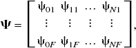
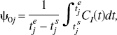
Example dictionaries (Ψ). (A) Plasma input basis. (B) Normalized plasma input basis. (C) Reference tissue input basis. (D) Normalized reference tissue input basis.

Solution of the general model by basis pursuit denoising

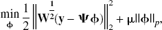
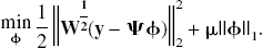
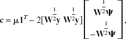
Standard least-squares techniques are not applicable because of the overcomplete basis, which leads to an underdetermined set of equations. This ill-posed problem requires an additional constraint to impose a unique solution on the estimation process. This constraint is chosen to be consistent with prior knowledge about the solution, namely, that the solution will be sparse in the basis coefficients. This constraint has also been used in the wavelet community, for the estimation of sparse representations from overcomplete dictionaries (Chen, 1995; Chen et al., 1999). The motivation for sparseness is consistent with the expectation that the data are accurately described by a few compartments (such as the models in Fig. 1). To transform the problem so that a unique solution exists, it is necessary to change the metric from ordinary least squares. The introduction of a regularizer or penalty function to the standard least-squares metric offers a framework for this,

min_{ϕ} \frac{1}{2} {‖ W^{\frac{1}{2}} (y - Ψ ϕ) ‖}_{2}^{2} + μ ‖ ϕ ‖_{p},

(16)

where the regularization parameter μ(>0) controls the tradeoff between approximation error and sparseness, Ψ is the overcomplete basis, φ are the basis coefficients to be determined, and y is the observed data. The addition of an L_p norm to the standard L2 norm in Eq. 16 allows for a uniquely determined parameter estimation process. Some possible choices for L_p are L₀ (atomic decomposition), L₁ (basis pursuit denoising), and L₂ (ridge regression) (Chen, 1995). The three regularizers have different characteristics and implementations. Both atomic decomposition and basis pursuit denoising promote a sparse solution which is consistent with our expectation of a compartmental model consisting of just a few tissue compartments, whereas ridge regression will encourage all parameters to be nonzero. Atomic decomposition is computationally demanding owing to its combinatorial nature. Both basis pursuit denoising and ridge regression can be constructed in a quadratic programming framework. Given these factors, a good choice for the estimation process is basis pursuit denoising, because this balances both a sparse solution with a computationally feasible parameter estimation approach. The basis pursuit denoising solution to the problem is presented here,

min_{ϕ} \frac{1}{2} {‖ W^{\frac{1}{2}} (y - Ψ ϕ) ‖}_{2}^{2} + μ ‖ ϕ ‖_{1} .

(17)

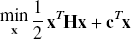
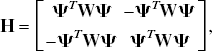
With the introduction of slack variables, basis pursuit denoising can be written as a simple bound constrained quadratic program (Chen, 1995; Chen et al., 1999):

min_{x} \frac{1}{2} x^{T} H x + c^{T} x

(18)

such that x_i ≥ 0 and where

H = [\begin{array}{l} Ψ^{T} W Ψ & - Ψ^{T} W Ψ \\ - Ψ^{T} W Ψ & Ψ^{T} W Ψ \end{array}],

(19)

c = μ 1^{T} - 2 [W^{\frac{1}{2}} y W^{\frac{1}{2}} y] [\begin{matrix} W^{\frac{1}{2}} Ψ \\ - W^{\frac{1}{2}} Ψ \end{matrix}],

(20)

x = [ϕ^{+} ϕ^{-}] .

(21)

The basis coefficients are given by

ϕ = ϕ^{+} - ϕ^{-} .

(22)

The quadratic program can be solved readily using standard optimizers (Mészáros, 1998). Thus, given a suitable regularization parameter, the general compartmental model can be fitted to the data. A method that allows the selection of an appropriate regularization parameter is now considered.

Selection of the regularization parameter. Basis pursuit denoising requires the determination of the regularization parameter, μ, for the penalty term. Here, this is obtained by the method of leave one out cross-validation (LOOCV) (Shao, 1993; Hjorth, 1994). LOOCV is a “resampling” method that allows the generalization error to be estimated. Fits are performed in which each data point is omitted in turn, and the generalization error is then estimated by summing up the prediction error for each omitted data point. The regularization parameter, μ, is chosen to minimize this estimate (Fig. 3). To achieve a more robust estimate of the most appropriate μ value, LOOCV is applied to a set of time–activity curves and the mean μ value is selected.

FIG. 3.

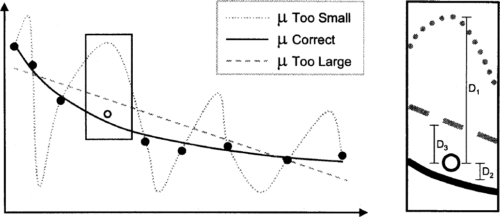
Effect of the regularization parameter (μ) and selection via leave one out cross-validation (LOOCV): When the μ value is too small, the data (•) are overfitted, and when the value is too big the data are underfitted. The “best” μ value is chosen using the method of LOOCV. A data point is omitted (○) and the data are fit for a set of μ values. The error in the model's prediction of the omitted data point is then calculated in a least-squares sense (i.e., D_i²). This is repeated for the omission of each data point in turn, and the resultant generalization errors are summated. A μ is selected by choosing the value of μ that minimizes this generalization error. The figure shows how the parsimonious model minimizes the generalization error (i.e., D₂² < D₃² < D₁²).

Model order and transparency

The presented method is transparent because it returns information about the underlying compartmental structure. The number of nonzero coefficients returned corresponds to the model order, which is related to the number of tissue compartments. The number of nonzero components is counted as the number of distinct peaks within the spectrum. The method will often include two peaks next to each other in order to approximate an exponential in between them. This occurrence is treated as a single nonzero coefficient. For plasma input models, the model order equals the number of tissue compartments (ignoring the blood volume component) and for reference tissue models, the number of nonzero coefficients corresponds to the total number of tissue compartments in the reference and target tissues. Although the model order dictates the number of compartments, any decision about the true model configuration is limited by the problem of indistinguishability. Figures 4 and 5 depict the sets of models that are equivalent in terms of model order for plasma input and reference tissue input models. If one requires a compartmental description of the tracer, and the set is not singular, then it is necessary to invoke biologic information about the system in order to select among the possible models.

FIG. 4.

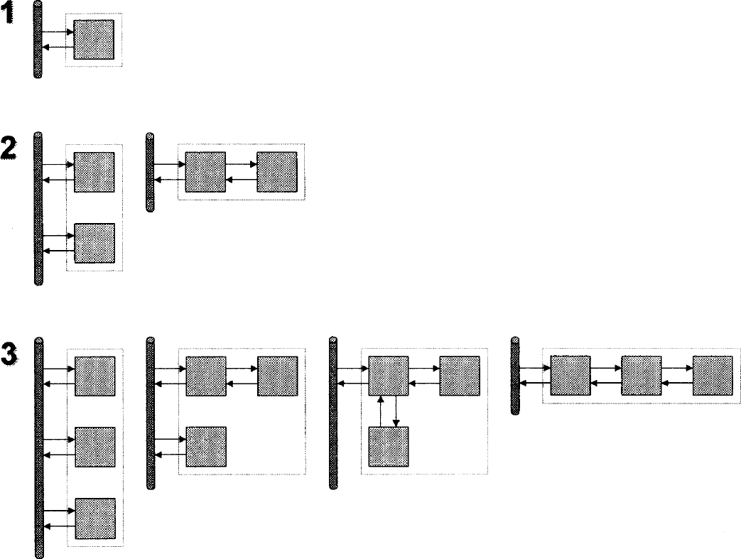
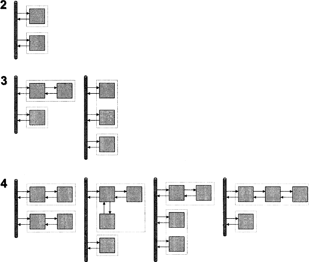
Indistinguishability for plasma input models. (top) Model order = 1: One possible configuration. (middle) Model order = 2: Two possible configurations. (bottom) Model order = 3: Four possible configurations.

FIG. 5.

Indistinguishability for reference tissue input models. (top) Model order = 2: One possible configuration. (middle) Model order = 3: Four possible configurations. (bottom) Model order = 4: Seven possible configurations. (There are up to twice as many possible configurations than are shown, as the reference and target tissues may be reversed.)

MATERIALS AND METHODS

For DEPICT and spectral analysis, the tissue and plasma data were uncorrected for the decay of the isotope. Instead, a decay constant was allowed for in the exponential coefficients (decay constant for [¹¹C]: λ = 0.034 min⁻¹). For the Logan analysis, the tissue and plasma data were precorrected for the decay of the isotope.

DEPICT

The basis pursuit denoising approach was implemented with 30 basis functions (logarithmically spaced between 0.048 and 6 min⁻¹). The number of basis functions was chosen to be 30 based on a balance between precision and computation time (data not shown). The weighting matrix was determined from the true TAC activity and the frame duration as described previously (Gunn et al., 1997). The regularization parameter, μ, was determined by numerically minimizing the LOOCV error across a discrete set of logarithmically spaced μ values (10^−3.5 ⩽ μ ⩽ 10^0.5). For the one-dimensional simulations, the parameter μ was determined as the mean value from the 1,000 realizations. For parametric imaging, the μ value was obtained from a series of LOOCV estimates (μ_i) obtained from random voxel locations contained within a brain mask. This process examined at least 20 voxels and continued until the relative precision of was less than 50%,

\frac{t_{0.975, d f} σ (μ)}{\sqrt{N} \bar{μ}} < 0.5,

(23)

where df is the degrees of freedom and is given by the length of μ – 1.

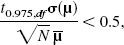
was then estimated as the mean of the vector μ. DEPICT is available at http://www.bic.mni.mcgill/∼rgunn.

Spectral analysis. Spectral analysis was implemented using the nonnegative least-squares algorithm (Cunningham and Jones, 1993) with the identical basis and weighting matrix as were used for DEPICT.

Logan analysis. The Logan analysis (Logan et al., 1990, 1996) was implemented as a linear regression of the transformed data after 45 minutes.

One-dimensional simulations

Simulations were performed to assess the stability of the three methods to different noise levels. A measured input function from a PET scan was used in conjunction with a two-tissue compartmental model to simulate noise-free data representative of a target tissue [K₁ = 0.4 (mL plasma) · min⁻¹ · (mL tissue)⁻¹, k₂ = 0.2 min⁻¹, k₃ = 0.4 min⁻¹ and k₄ = 0.1 min⁻¹) and a reference tissue [K′₁ = 0.4 (mL plasma) · min⁻¹ · (mL tissue)⁻¹, k′₂ = 0.4 min⁻¹, k′₅ = 1 min⁻¹ and k′₆ = 1 min⁻¹]. Ninety minutes of data were simulated for a total of 24 temporal frames (3 × 10 seconds, 3 × 20 seconds, 3 × 60 seconds, 5 × 120 seconds, 5 × 300 seconds, 5 × 600 seconds). The noise-free simulated data are shown in Fig. 6. For a range of noise levels, 1,000 realizations of noisy target tissue TACs were generated by adding normally distributed noise proportional to the activity/frame duration at each point. The noise variance was scaled so that a value of 1 corresponded to the largest noise-free TAC value. These data were then analyzed in two different ways: (1) using the plasma input function, the noisy target tissue TACs were fitted with the basis pursuit method, the Logan plot, and spectral analysis to derive V_D estimates; and (2) using the reference tissue input function, the noisy target tissue TACs were fitted with the basis pursuit method and the Logan plot to derive BP.f₂ estimates.

FIG. 6.

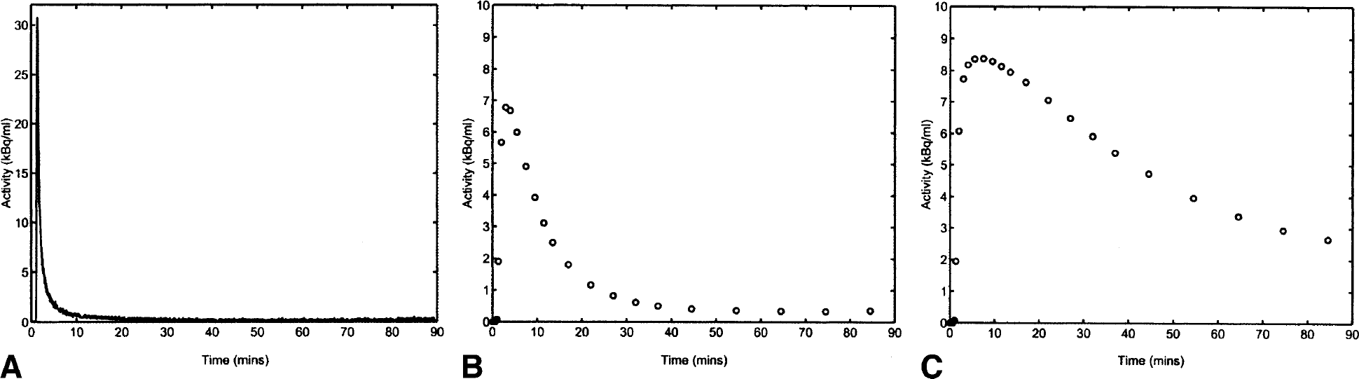
One-dimensional simulation data: noise-free time–activity curves (TAC). (A) Plasma input function. (B) Reference tissue TAC. (C) Target tissue TAC.

Four-dimensional simulations

Simulated dynamic PET data were generated using PETSim, a dynamic PET simulator (Ma et al., 1993; Ma and Evans, 1997) as described previously (Aston et al., 2000). In short, the simulator takes a magnetic resonance image volume segmented into 28 regions, each of which is assigned an activity value, and generates a simulated PET volume. The resolution and noise characteristics were chosen to correspond to the ECAT HR+ PET camera (CTI, Knoxville, TN, U.S.A.) in 3D mode with a resolution of 4 × 4 × 4.2-mm full width at half maximum (FWHM) at the center of the field of view and images were reconstructed using a 6-mm FWHM Hanning filter. A simulated [¹¹C]SCH 23390 data set was generated using a measured plasma input function and a two-tissue compartmental model to simulate regional tissue kinetics using rate constants for different brain regions taken from human PET data, K₁ (0.08 to 0.13 mL plasma · min⁻¹ mL tissue⁻¹), k₂ (0.24 to 0.37 min⁻¹), k₃ (0 to 0.14 min⁻¹), k₄ (0.1 min⁻¹) for 34 time frames (4 × 15 seconds, 4 × 30 seconds, 7 × 60 seconds, 5 × 120 seconds, 14 × 300 seconds). The cerebellum was simulated with a one-tissue compartment model. Two dynamic data sets were generated; a noise-free data set and the other consistent with an injection of 370 MBq of activity. The two data sets were analyzed with DEPICT to estimate parametric images of V_D and model order.

Measured data sets

Two measured data sets, which were taken from ongoing clinical studies (MRC Cyclotron Unit, Hammersmith Hospital, London, U.K.), were analyzed with DEPICT. Both data sets were acquired on the ECAT EXACT3D (CTI) (Spinks et al., 2000). The data were reconstructed with model-based scatter correction and measured attenuation correction using the method of filtered backprojection (ramp filter, 0.5 Nyquist). The reconstructed images had a resolution of 4.8 × 4.8 × 5.6 mm at the center of the field of view:

[¹¹C]Diprenorphine (opiate receptor): 130 MBq of the radioligand was injected into a normal male volunteer, and acquisition consisted of 32 temporal frames of data (1 × 50 seconds, 3 × 10 seconds, 7 × 30 seconds, 12 × 120 seconds, 6 × 300 seconds, 3 × 600 seconds). Continuous arterial sampling and metabolite analyses were performed during the scan, which allowed for the generation of a metabolite corrected plasma input function as described previously (Jones et al., 1994). DEPICT was used to estimate parametric images of V_D and model order using a plasma input analysis.

[¹¹C]WAY-100635 (5-HT1A receptor): 243 MBq of the radioligand was injected into a normal male volunteer and acquisition consisted of 22 temporal frames of data (1 × 15 seconds, 3 × 5 seconds, 2 × 15 seconds, 4 × 60 seconds, 7 × 300 seconds, 5 × 600 seconds). A region of interest was defined on the cerebellum for the extraction of a reference region TAC. DEPICT was used to estimate parametric images of BP.f₂ and model order using a reference tissue input analysis.

RESULTS

One-dimensional simulations

A summary of the results from the 1D noise simulations is presented in Fig. 7 for the plasma input model. DEPICT was able to obtain a good fit to the data. Both DEPICT and spectral analysis performed well in terms of parameter and model order estimation. Table 2 shows that DEPICT produces the lowest mean square error (MSE) of the three methods. The reference tissue input simulations are summarized in Fig. 8 and Table 3. Again DEPICT obtained a good fit to the data and a reasonable model order estimation. Table 3 shows that DEPICT produces the lowest MSE of the two methods.

TABLE 2.

One-dimensional simulation: summary parameters for V_D estimation with a plasma input function

Noise level		0	0.01	0.02	0.04	0.08	0.16	0.32	0.64
DEPICT		0.0001	0.0100	0.0120	0.0138	0.0328	0.0482	0.1990	0.4190
	MSE	0.0002	0.0004	0.0011	0.0036	0.0107	0.0267	0.0815	0.2190
Logan analysis	MSE	0.0123	0.0127	0.0137	0.0180	0.0356	0.1040	0.5670	0.9840
Spectral analysis	MSE	0.0089	0.0089	0.0093	0.0103	0.0149	0.0325	0.0942	0.2280

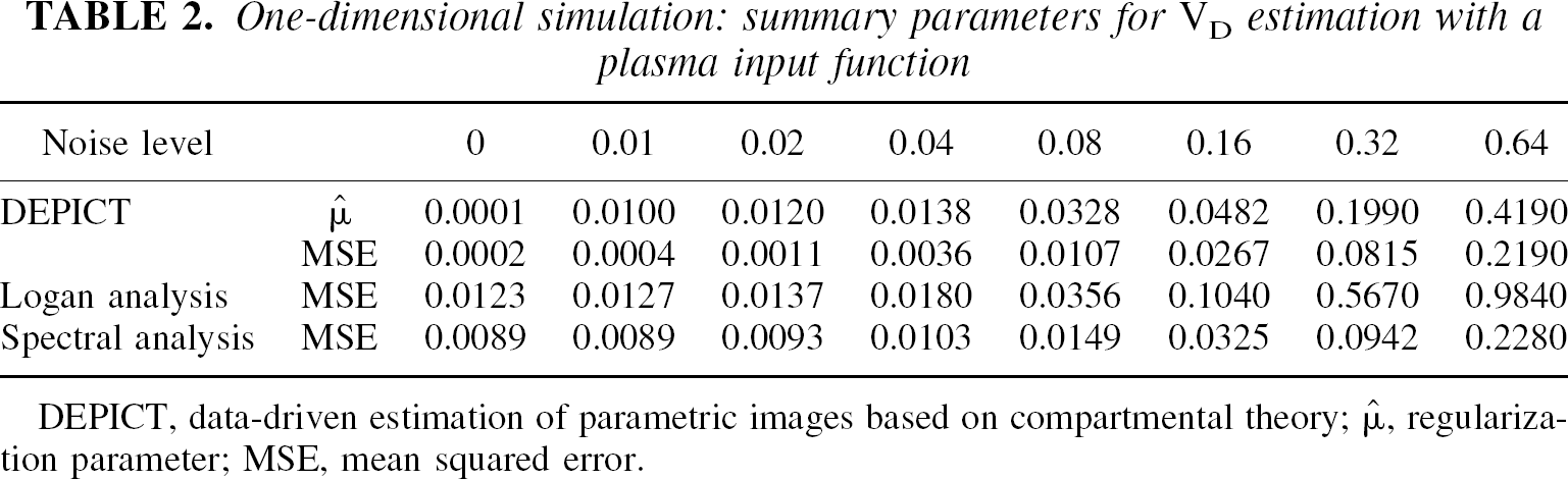
DEPICT, data-driven estimation of parametric images based on compartmental theory; , regularization parameter; MSE, mean squared error.

TABLE 3.

One-dimensional simulation: summary parameters for BP.f₂ estimation with a reference tissue input function

Noise level		0	0.01	0.02	0.04	0.08	0.16	0.32	0.64
DEPICT		0.0001	0.0010	0.0014	0.0026	0.0056	0.0187	0.0414	0.0869
	MSE	0.0077	0.0081	0.0085	0.0155	0.0356	0.1060	0.2790	0.8180
Logan analysis	MSE	0.0108	0.0128	0.0167	0.0345	0.1230	0.4040	1.7400	4.1400

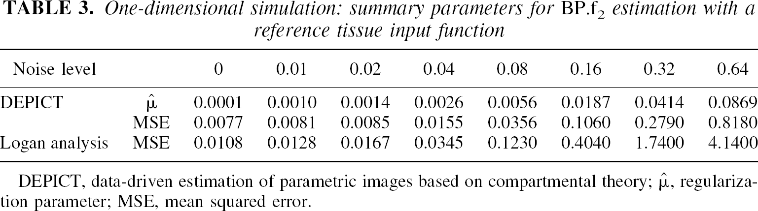
DEPICT, data-driven estimation of parametric images based on compartmental theory; , regularization parameter; MSE, mean squared error.

FIG. 7.

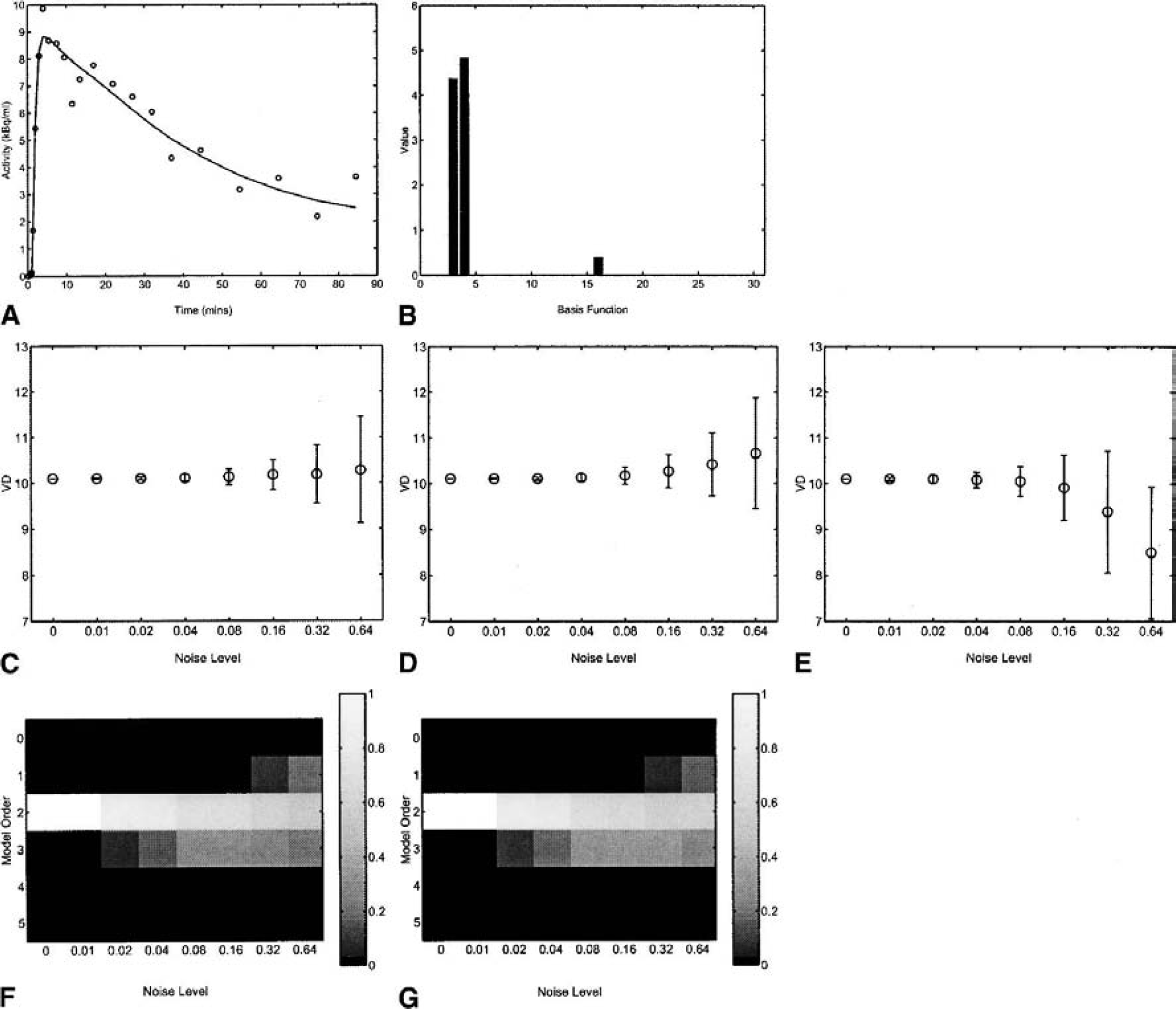
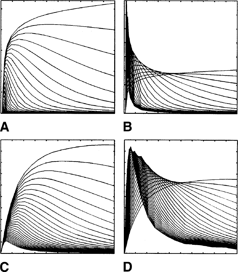
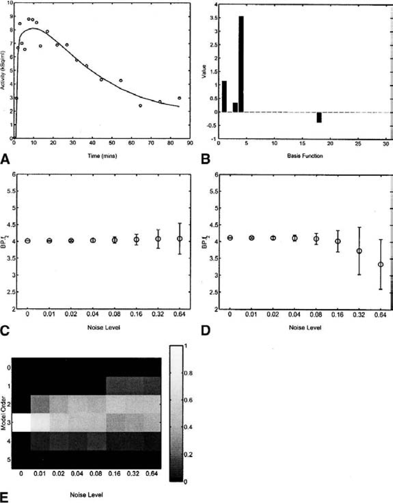
One-dimensional simulation: plasma analysis. (A) Example data-driven estimation of parametric images based on compartmental theory (DEPICT) fit; (B) DEPICT spectrum from fit in A; (C) DEPICT V_D; (D) spectral analysis V_D; (E) Logan analysis V_D; (F) DEPICT model order; and (G) spectral analysis model order. In subfigures (F) and (G) the color bar indicates the fraction of fits that corresponded to a particular model order.

FIG. 8.

One-dimensional simulation: reference tissue analysis. (A) Example data-driven estimation of parametric images based on compartmental theory (DEPICT) fit; (B) DEPICT spectrum from fit in A; (C) DEPICT BP.f₂; (D) Logan analysis BP.f₂; and (E) DEPICT model order. In subfigure (E) the color bar indicates the fraction of fits that corresponded to a particular model order.

Four-dimensional simulations

Parametric images estimated from the noisy 4D realization using DEPICT were of good quality and are presented in Fig. 9. DEPICT accurately estimates the number of tissue compartments used in the simulation (Fig. 9B), with two tissue compartments estimated on average within the cortical regions and one tissue compartment on average within the cerebellum.

The regularization parameter was calculated as = 0.045 (Fig. 10A). DEPICT was also applied to the noise-free data set, and this allowed for the calculation of the percentage error in the V_D estimate. The error distribution is given in Fig. 10B.

FIG. 9.

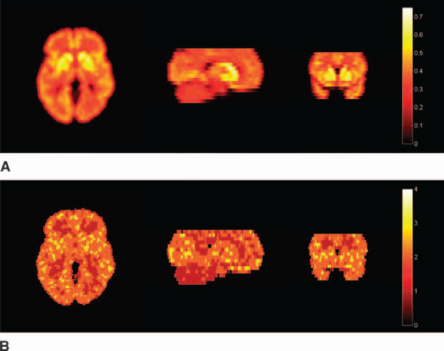
Four-dimensional simulation: parametric images estimated using DEPICT. (A) V_D image. (B) Model order image.

FIG. 10.

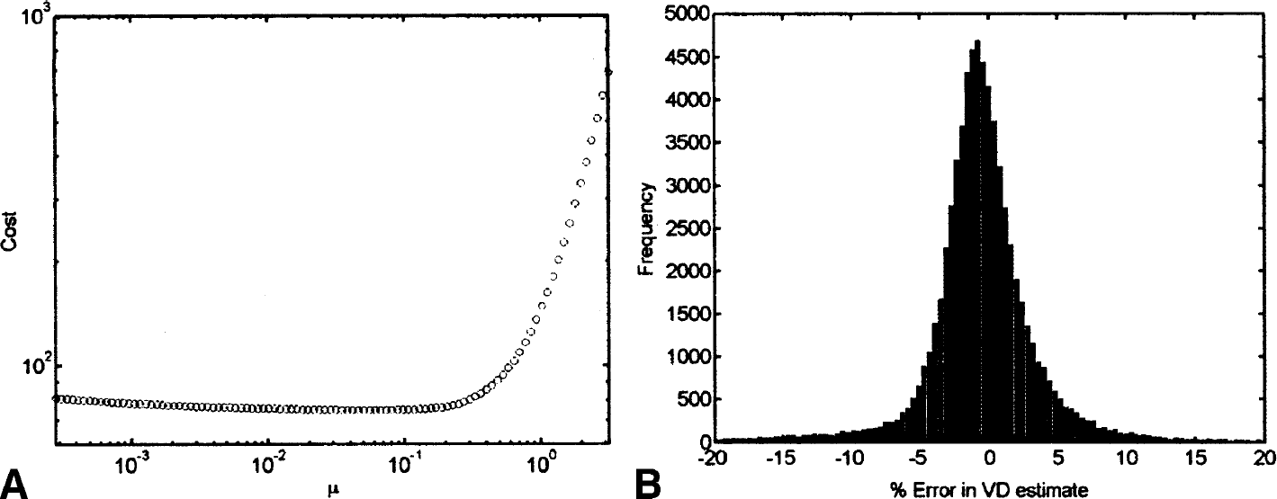
Four-dimensional simulation: cost function and error in V_D estimate. (A) Cost function for regularization parameter (μ). (B) Percent error of V_D estimate shown in Fig. 9.

Measured data

Both the parametric images of V_D for [¹¹C]diprenorphine and BP.f₂ for [¹¹C]WAY-100635 were of good quality and reflected the known distribution of opiate and 5-HT1A receptor sites, respectively. The model order images for both radioligands showed less structure than the 4D simulation, but both reflected the model order expected for [¹¹C]diprenorphine (Jones et al., 1994) and [¹¹C]WAY-100635 (Gunn et al., 1998; Farde et al., 1998; Parsey et al., 2000) (Fig. 11). These parametric images took 1 hour to compute with DEPICT on a desktop workstation (equivalent computation times for parametric images generated by the Logan analysis and Spectral analysis would be 5 minutes and 30 minutes, respectively). The regularization parameters were calculated as = 0.0095 for [¹¹C]diprenorphine and = 0.015 for [¹¹C]WAY-100635 (Fig. 12).

FIG. 11.

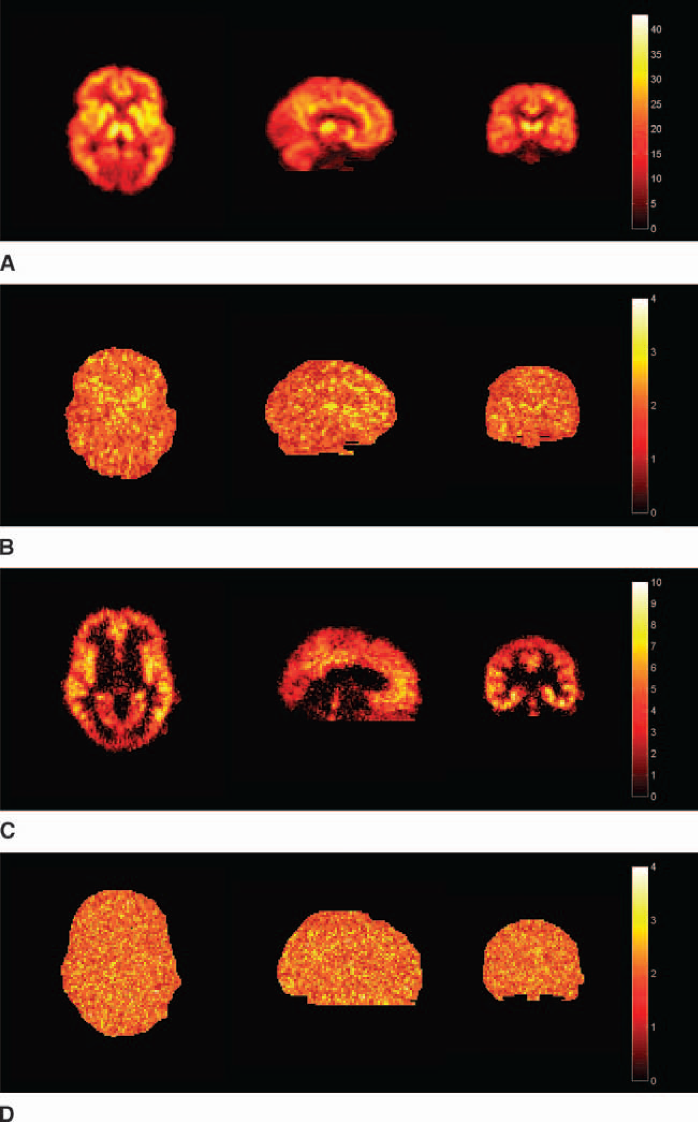
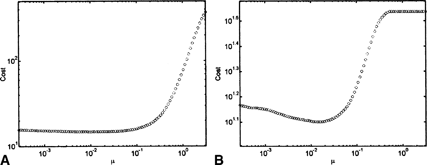
Measured data: parametric images estimated using data-driven estimation of parametric images based on compartmental theory (DEPICT). (A) [¹¹C]Diprenorphine: V_D image. (B) [¹¹C]Diprenorphine: model order image. (C) [¹¹C]WAY-100635: BP.f₂ image. (D) [¹¹C]WAY-100635: model order image.

FIG. 12.

Measured data: cost functions for regularization parameter (μ). (A) [¹¹C]Diprenorphine. (B) [¹¹C]WAY-100635.

DISCUSSION

The current article has introduced DEPICT, a tracer kinetic modeling technique for the quantitative analysis of dynamic in vivo radiotracer studies that allows for the data-driven estimation of parametric images based on compartmental theory. DEPICT requires no a priori decision about the tracers fate in vivo, instead determining the most appropriate model from the information contained within the data. Although the method is classed as data-driven, it is founded on compartmental theory (Gunn et al., 2001) and this enables parameter estimates to be interpreted within a traditional compartmental framework. The system macro parameters are simply determined from the estimated IRF. The method can be applied to dynamic radiotracer studies involving either a bolus or bolus-infusion tracer administration scheme. DEPICT is general, and although the examples here are concerned with tracers exhibiting reversible kinetics, the method is equally applicable to systems with irreversible kinetics. In addition to parameter estimates, DEPICT returns model order estimates that correspond to the number of numerically identifiable compartments in the system. There may be additional compartments that are not supported by the statistical quality of the data; however, this is not in any way a practical restriction.

DEPICT uses a basis function approach (Koeppe et al., 1985; Cunningham and Jones, 1993; Gunn et al., 1997) to the parameter estimation problem. The constructed problem is ill posed, and its solution requires an appropriate constraint. Spectral analysis approaches this problem using the nonnegative least-squares algorithm (Cunningham and Jones, 1993), whereas DEPICT uses the method of basis pursuit denoising (Chen, 1995), which involves a one-norm penalty function on the coefficients. Both methods lead to a sparse solution, but DEPICT does not constrain the coefficients to be positive, which makes it appropriate for application to the general reference tissue model. Basis pursuit denoising is a technique that extracts a subset of terms from an overcomplete dictionary, and thus it is possible to provide a model that is interpretable, while retaining good approximating capability. The principle behind the approach is to trade off the error in approximation with the sparseness of the representation.

The three data-driven methods investigated all performed well for low noise levels, as determined from the 1D simulations, with DEPICT returning the lowest mean squared error. The Logan analysis demonstrated a bias at higher noise levels, which has been documented recently (Slifstein and Laruelle, 2000). To address the issue of noise-induced bias in the Logan analysis, two approaches have since been developed (Logan et al., 2001; Varga and Szabo, 2002). These modifications would have improved the performance of the Logan analysis at high noise levels but were not considered here, because the aim was to introduce DEPICT and compare it against the data-driven methods in common use. DEPICT and spectral analysis allow for the estimation of the model order. The model order was well characterized by both methods for the 1D plasma input simulations and using DEPICT for the reference tissue input simulations. Spectral analysis is not valid for the general reference tissue model because it does not permit negative coefficients, which can occur in the impulse response function.

In summary, this article has introduced a new method, DEPICT, which delivers parametric images or regional parameter estimates from dynamic radiotracer imaging studies without the need to specify a compartmental structure. DEPICT is applicable to both plasma and reference tissue input analyses. The results presented demonstrate that DEPICT is highly competitive with existing data-driven estimation methods. Furthermore, DEPICT is a transparent data-driven modeling approach because it returns not only macro parameter values, but also information on the underlying model structure.

Footnotes

1

Here, the blood volume term for plasma input models is treated as a plasma volume term (i.e., C_B(t) = C_P(t)) which enables us to express both the plasma and reference tissue input cases in the same framework. This is simply so that we may be concise in our notation. To use a whole blood volume term Ψ₀ = C_P is replaced by Ψ₀ = C_B in .

APPENDIX A: LOGAN PLOT DERIVATION

Here, a formal derivation of the Logan plot is presented for both a plasma and reference tissue input function. The plasma input Logan plot corresponds to the original presentation by Logan et al. (1990). The reference tissue input analysis presented here differs from Logan et al. (1996) in that it proves that the plot is valid for an arbitrary number of compartments in the reference tissue as well as the target tissue. Both derivations presented exclude the presence of vascular contribution to the tissue signal.

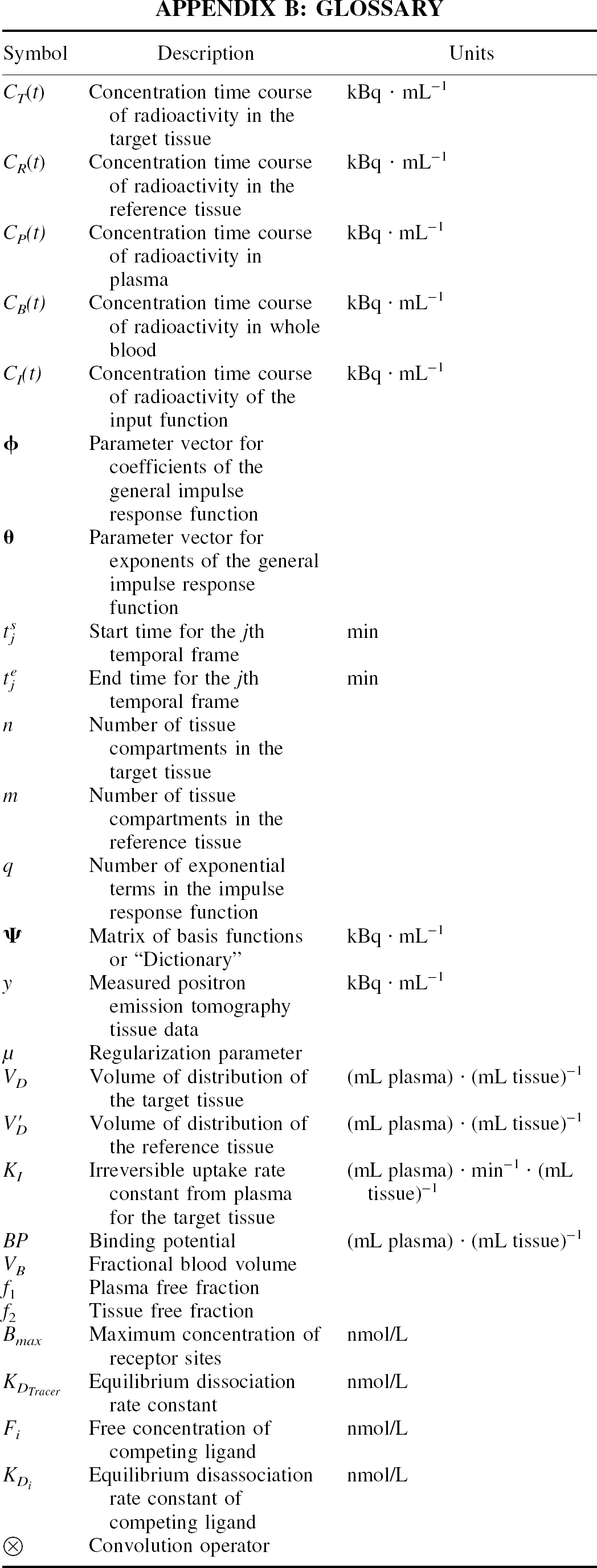
APPENDIX B: GLOSSARY

Symbol	Description	Units
Cj(t)	Concentration time course of radioactivity in the target tissue	kBq · mL⁻¹
C_R(t)	Concentration time course of radioactivity in the reference tissue	kBq · mL⁻¹
C_p(t)	Concentration time course of radioactivity in plasma	kBq · mL⁻¹
C_B(t)	Concentration time course of radioactivity in whole blood	kBq · mL⁻¹
C(t)	Concentration time course of radioactivity of the input function	kBq · mL⁻¹
ϕ	Parameter vector for coefficients of the general impulse response function
θ	Parameter vector for exponents of the general impulse response function
t^s_j	Start time for the jth temporal frame	min
t^e_j	End time for the jth temporal frame	min
n	Number of tissue compartments in the target tissue
m	Number of tissue compartments in the reference tissue
q	Number of exponential terms in the impulse response function
Ψ	Matrix of basis functions or “Dictionary”	kBq · mL⁻¹
y	Measured positron emission tomography tissue data	kBq · mL⁻¹
μ	Regularization parameter
V_D	Volume of distribution of the target tissue	(mL plasma) · (mL tissue)⁻¹
V′_D	Volume of distribution of the reference tissue	(mL plasma) · (mL tissue)⁻¹
K_I	Irreversible uptake rate constant from plasma for the target tissue	(mL plasma) · min⁻¹ · (mL tissue)⁻¹
BP	Binding potential	(mL plasma) · (mL tissue)⁻¹
V_B	Fractional blood volume
f ₁	Plasma free fraction
f ₂	Tissue free fraction
B_max	Maximum concentration of receptor sites	nmol/L
K_DTracer	Equilibrium dissociation rate constant	nmol/L
F_i	Free concentration of competing ligand	nmol/L
K_Di	Equilibrium disassociation rate constant of competing ligand	nmol/L
⊗	Convolution operator

References

Aston

JAD

Gunn

Worsley

Evans

Dagher

(2000) A statistical method for the analysis of positron emission tomography neuroreceptor ligand data. Neuroimage 12:245–256

Blomqvist

Pauli

Farde

Ericksson

Persson

Halldin

(1989) Dynamic models of reversible ligand binding. In: Clinical research and clinical diagnosis ( Beckers

Goffinet

Bol

, eds), Dardrecht, The Netherlands: Kluwer Academic Publishers, pp 35–44

Carson

(1986) Parameter estimation in positron emission tomography. In: Positron emission tomography and autoradiography: Principles and applications for the brain and heart ( Phelps

Mazziotta

Shelbert

, eds), New York: Raven Press, pp 347–390

Carson

Huang

Green

(1986) Weighted integration method for local cerebral blood flow measurements with positron emission tomography. J Cereb Blood Flow Metab 6:245–258

Chen

(1995) Basis pursuit [Ph.D. thesis]. Stanford, CA: Dept. of Statistics, Stanford University

Chen

Donoho

Saunders

(1999) Atomic decomposition by basis pursuit. SIAM J Sci Computing 20:33–61

Cunningham

Hume

Price

Ahier

Cremer

Jones

(1991) Compartmental analysis of diprenorphine binding to opiate receptors in the rat in vivo and its comparison with equilibrium data in vitro. J Cereb Blood Flow Metab 11:1–9

Cunningham

Jones

(1993) Spectral analysis of dynamic PET studies. J Cereb Blood Flow Metab 13:15–23

Cunningham

Gunn

Byrne

Matthews

(1998) Suppression of noise artefacts in spectral analysis of dynamic PET data. In: Quantitative functional brain imaging with positron emission tomography ( Carson

Daube-Witherspoon

Herscovitch

, eds), San Diego: Academic Press, pp 329–337

10.

Farde

Ito

Swahn

Pike

Halldin

(1998) Quantitative analyses of carbonyl-carbon-11-WAY-100635 binding to central 5-hydroxytryptamine-1A receptors in man. J Nucl Med 39:1965–1971

11.

Feng

Huang

Wang

(1996) An unbiased parametric imaging algorithm for uniformly sampled biomedical system parameter estimation. IEEE Trans Med Imag 15:512–518

12.

Gjedde

(1982) Calculation of cerebral glucose phosphorylation from brain uptake of glucose analogs in vivo: A re-examination. Brain Res Rev 4:237–274

13.

Gunn

Lammertsma

Hume

Cunningham

(1997) Parametric imaging of ligand-receptor binding in PET using a simplified reference region model. Neuroimage 6:279–287

14.

Gunn

Sargent

Bench

Rabiner

Osman

Pike

Hume

Grasby

Lammertsma

(1998) Tracer kinetic modeling of the 5-HT1A receptor ligand [carbonyl-11C]WAY-100635 for PET. Neuroimage 8:426–440

15.

Gunn

Cunningham

(2001) Positron emission tomography compartmental models. J Cereb Blood Flow Metab 21:635–652

16.

Hjorth

JSU

(1994) Computer intensive statistical methods validation, model selection, and bootstrap. London: Chapman & Hall

17.

Huang

Phelps

(1986) Principles of tracer kinetic modeling in positron emission tomography and autoradiography. In: Positron emission tomography and autoradiography: Principles and applications for the brain and heart. New York: Raven Press, pp 287–346

18.

Hume

Myers

Bloomfield

Opacka-Juffry

Cremer

Ahier

Luthra

Brooks

Lammertsma

(1992) Quantitation of carbon-11-labeled raclopride in rat striatum using positron emission tomography. Synapse 12:4754

19.

Jones

Cunningham

Ha-Kawa

Fujiwara

Liyii

Luthra

Ashburner

Osman

Jones

(1994) Quantitation of [11C]diprenorphine cerebral kinetics in man acquired by PET using presaturation, pulse-chase and tracer-only protocols. J Neurosci Methods 51:123–134

20.

Kety

(1951) The theory and application of the exchange of inert gases at the lungs and tissues. Pharmacol Rev 3:1–41

21.

Koeppe

Holden

(1985) Performance comparison of parameter estimation techniques for the quantitation of local cerebral blood flow by dynamic positron computed tomography. J Cereb Blood Flow Metab 5:224–234

22.

Lammertsma

Hume

(1996) Simplified reference tissue model for PET receptor studies. Neuroimage 4:153–8

23.

Lammertsma

Bench

Hume

Osman

Gunn

Brooks

Frackowiak

(1996) Comparison of methods for analysis of clinical [11C]raclopride studies. J Cereb Blood Flow Metab 16:42–52

24.

Laruelle

(2000) Imaging synaptic neurotransmission with in vivo binding competition techniques: A critical review. J Cereb Blood Flow Metab 20:423–451

25.

Logan

Fowler

Volkow

Wolf

Dewey

Schlyer

MacGregor

Hitzemann

Bendriem

Gatley

Christman

(1990) Graphical analysis of reversible radioligand binding from time-activity measurements applied to [N-11C-methyl]−(−)−cocaine PET studies in human subjects. J Cereb Blood Flow Metab 10:740–747

26.

Logan

Fowler

Volkow

Wang

G-J

Ding

Y-S

Alexoff

(1996) Distribution volume ratios without blood sampling from graphical analysis of PET data. J Cereb Blood Flow Metab 18:834–840

27.

Logan

Fowler

Volkow

Ding

Wang

Alexoff

(2001) A strategy for removing the bias in the graphical analysis method. J Cereb Blood Flow Metab 21:307–320

28.

Evans

(1997) Analytical modeling of PET imaging with correlated functional and structural images. IEEE Trans Nucl Sci 44:2439–2444

29.

Kamber

Evans

(1993) 3D simulation of PET brain images using segmented MRI data and positron tomograph characteristics. Comput Med Imaging Graph 17:365–371

30.

Mazoyer

Huesman

Budinger

Knittel

(1986) Dynamic PET data analysis. J Comput Assist Tomogr 10:645–653

31.

Mészáros

(1998) The BPMPD interior point solver for convex quadratic problems. Technical Report WP 98–8. Budapest: Computer and Automation Research Institute, Hungarian Academy of Sciences

32.

Mintun

Raichle

Kilbourn

Wooten

Welch

(1984) A quantitative model for the in vivo assessment of drug binding sites with positron emission tomography. Ann Neurol 15:217–227

33.

Parsey

Slifstein

Hwang

Abi-Dargham

Simpson

Mawlawi

Guo

Van Heertum

Mann

Laruelle

(2000) Validation and reproducibility of measurement of 5-HT1A receptor parameters with [carbonyl-11C]WAY-100635 in humans: Comparison of arterial and reference tissue input functions. J Cereb Blood Flow Metab 20:1111–1133

34.

Patlak

Blasberg

(1985) Graphical evaluation of blood-to-brain transfer constants from multiple-time uptake data: Generalizations. J Cereb Blood Flow Metab 5:584–590

35.

Patlak

Blasberg

Fenstermacher

(1983) Graphical evaluation of blood-to-brain transfer constants from multiple-time uptake data. J Cereb Blood Flow Metab 3:1–7

36.

Phelps

Huang

Hoffman

Selin

Sokoloff

Kuhl

(1979) Tomographic measurement of local cerebral glucose metabolic rate in humans with (F-18)2-fluoro-2-deoxy-D-glucose: Validation of method. Ann Neurol 6:371–388

37.

Schmidt

(1999) Which linear compartmental systems can be analyzed by spectral analysis of PET output data summed over all compartments? J Cereb Blood Flow Metab 19:560–569

38.

Shao

(1993) Linear model selection by cross-validation. J Am Stat Assoc 88:486–494

39.

Slifstein

Laruelle

(2000) Effects of statistical noise on graphic analysis of PET neuroreceptor studies. J Nucl Med 41:2083–2088

40.

Sokoloff

Reivich

Kennedy

DesRosiers

Patlak

Pettigrew

Sakurada

Shinohara

(1977) The 14C-deoxyglucose method for the measurement of local cerebral glucose utilisation: Theory, procedure and normal values in the conscious and anesthetized albino rat. J Neurochem 28:897–916

41.

Spinks

Jones

Bloomfield

Bailey

Miller

Hogg

Jones

Vaigneur

Reed

Young

Newport

Moyers

Casey

Nutt

(2000) Physical characteristics of the ECAT EXACT3D positron tomograph. Phys Med Biol 45:2601–2618

42.

Varga

Szabo

(2002) Modified regression model for the Logan plot. J Cereb Blood Flow Metab 22:240–244

43.

Watabe

Carson

Iida

(2000) The reference tissue model: Three compartments for the reference region. NeuroImage 11:S12

Positron Emission Tomography Compartmental Models: A Basis Pursuit Strategy for Kinetic Modeling

Abstract

Keywords

THEORY

Plasma input models

Reference tissue input models

Parameters for neuroreceptor binding studies

Construction of the general model in a basis function framework

Solution of the general model by basis pursuit denoising

Model order and transparency

MATERIALS AND METHODS

DEPICT

One-dimensional simulations

Four-dimensional simulations

Measured data sets

RESULTS

One-dimensional simulations

Four-dimensional simulations

Measured data

DISCUSSION

Footnotes

1

APPENDIX A: LOGAN PLOT DERIVATION

APPENDIX B: GLOSSARY

References