
Abstract
The current article presents theory for compartmental models used in positron emission tomography (PET). Both plasma input models and reference tissue input models are considered. General theory is derived and the systems are characterized in terms of their impulse response functions. The theory shows that the macro parameters of the system may be determined simply from the coefficients of the impulse response functions. These results are discussed in the context of radioligand binding studies. It is shown that binding potential is simply related to the integral of the impulse response functions for all plasma and reference tissue input models currently used in PET. This article also introduces a general compartmental description for the behavior of the tracer in blood, which then allows for the blood volume-induced bias in reference tissue input models to be assessed.
Compartmental analysis forms the basis for tracer kinetic modeling in positron emission tomography (PET). Well-established compartmental models in PET include those used for the quantification of blood flow (Kety, 1951), cerebral metabolic rate for glucose (Sokoloff et al., 1977; Phelps et al., 1979), and neuroreceptor ligand binding (Mintun et al., 1984). These particular models require an arterial blood or plasma input function, with the number of tissue compartments dictated by the physiological, biochemical and pharmacological properties of the system under study. Other “reference tissue models” have been developed, particularly for the study of neuroreceptor ligands (Blomqvist et al., 1989; Cunningham et al., 1991; Hume et al., 1992; Lammertsma et al., 1996; Lammertsma and Hume, 1996; Gunn et al., 1997; Watabe et al., 2000), with a view to avoiding blood sampling. These enable the target tissue time-activity curve to be expressed as a function of that of the reference tissue. For neuroreceptor applications, reference tissue models assume that there exists a reference area of brain tissue essentially devoid of specific binding sites. The number of identifiable compartments in the reference region and in the region of interest is dependent on the rate of exchange of the tracer between the free, nonspecifically bound and specifically bound pools of tracer. All of these models make a series of general assumptions—for example, that there is instantaneous mixing within the individual compartments, and that the concentration of tracer is small enough such that it does not perturb the system under study. Under these conditions the systems are described by a set of first order linear differential equations. Parameter estimates may be obtained by the weighted least squares fitting of these models to measured PET data. The current article is not concerned with the determination of model complexity from measured data, but rather with the analysis of those model configurations that have been selected a priori by the investigator.
In PET, the measured regional radioactivity comprises the sum of all tissue compartments and a blood volume component. As Schmidt (1999) comments, “most of the literature on compartmental systems has been concerned with measurement of the content of individual compartments, and little attention has been directed to the particular problem of characterizing the sum of the contents in all compartments of the system.” The current article is principally concerned with developing a general framework for PET compartmental models. It aims to draw attention to the parallels that exist between reference tissue models and those models using a plasma input, and to those properties of reference tissue models that are robust and common to all models independent of the number and topology of compartments used to describe the tissues. Both reversible and irreversible systems will be considered and particular attention will be paid to their interpretation in terms of neuroreceptor ligand binding studies.
The current article presents general theory for modeling of tissue data using either plasma input or a reference tissue input. Theory is also presented for the behavior of the tracer in blood that accounts for both partitioning and metabolism (Appendix A). This enables theoretical consideration of blood activity contribution to the tissue signals for reference tissue input models. General theory is derived that gives the explicit functional form for the impulse response functions of the systems. It will be shown that simple relations exist between these functional forms and the macro system parameters. But first, the authors introduce some of the basic concepts used in this article.
Linear compartmental systems
Linear compartmental systems lead to a set of first order differential equations. Often in PET articles these equations are written out explicitly; however, it is convenient and concise to represent the whole system in terms of its state space representation. A time-invariant linear compartmental system is defined in terms of its state space representation as,
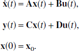
where
Macro and micro parameters
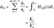
In the current article, the terms macro and micro parameters are used to distinguish between the individual rate constants (micro) and global system parameters that are functions of the rate constants (macro). For instance, the volume of distribution of the target tissue, VD, which is equal to the step response of the system, and the irreversible uptake rate constant from plasma, KI, which is equal to the steady state response of the system are both macro parameters. The macro parameters are generally more stable with respect to the parameter estimation problem from dynamic PET data.
Indistinguishability and identifiability
The current article discusses the concepts of indistinguishability and identifiability of the linear compartmental systems. Indistinguishability is concerned with determining a set of models that give rise to identical input–output behavior. Structural identifiability is concerned with whether the parameters may be estimated uniquely from perfect input–output data. This may be determined from analysis of the transfer function using a technique such as the Laplace transform approach (Godfrey, 1983).
PLASMA INPUT MODELS
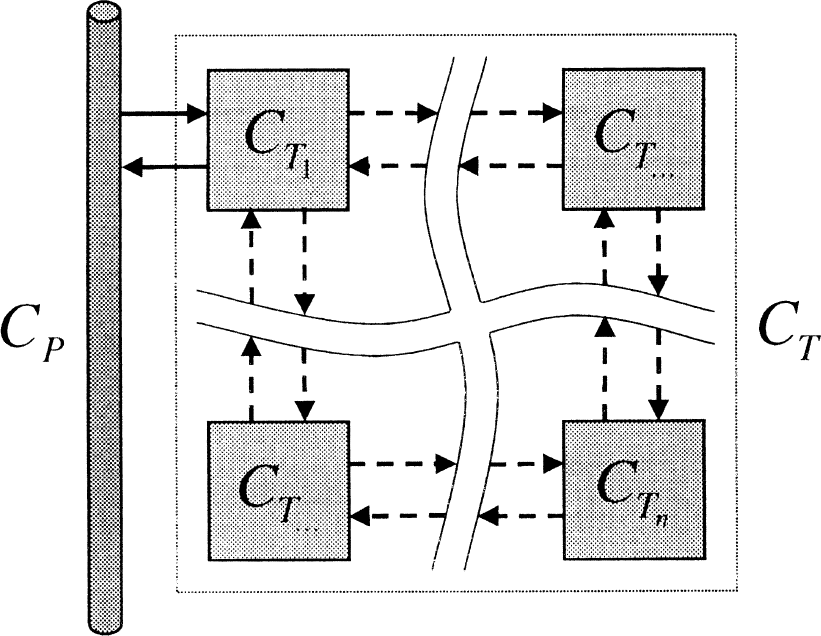
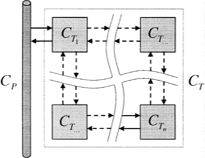
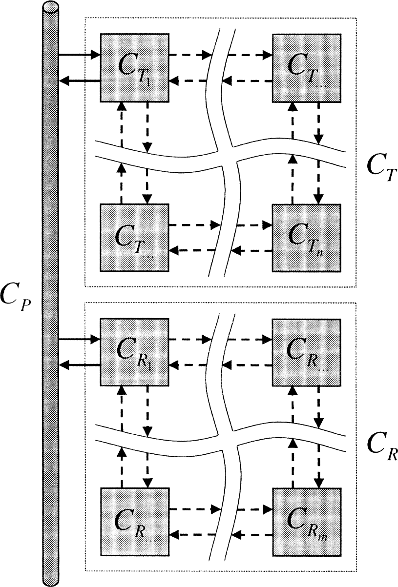
Consider a general PET system, as illustrated in Fig. 1, in which the measured radioactivity data consists of the total tissue concentration, CT, the parent tracer concentration in plasma, CP, and the whole blood concentration, CB. The blood volume component is omitted from Fig. 1 for clarity.
Its state space formulation is given by
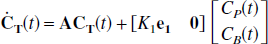
Generalized tissue model.
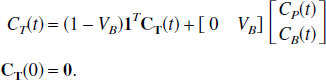
where
Definition 1
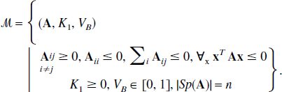
Let M denote the set of linear compartmental systems with n compartments (described by Eq. 2.1), where
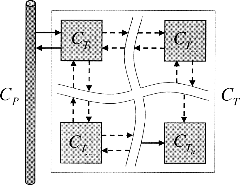
Let R denote the set of reversible models (Fig. 2),

Reversible tissue model.
and I denote the set of irreversible models with a single trap 2 (Fig. 3),
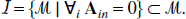
Irreversible tissue model with a single trap.
Theorem 1
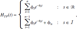
A model s εM has a solution given by,

where
θ
i
> 0 and
If s εR,
If s εI,
It is straightforward to derive an indistinguishability and indentifiability corollary directly from Theorem 1.
Corollary 1.1
Indistinguishability: any two plasma input models within the subset R (or similarly for I) with a total of N tissue compartments are indistinguishable.
Corollary 1.2
Identifiability: the macro parameters (K1, VD or KI) are uniquely identifiable from perfect input–output data.
REFERENCE TISSUE INPUT MODELS
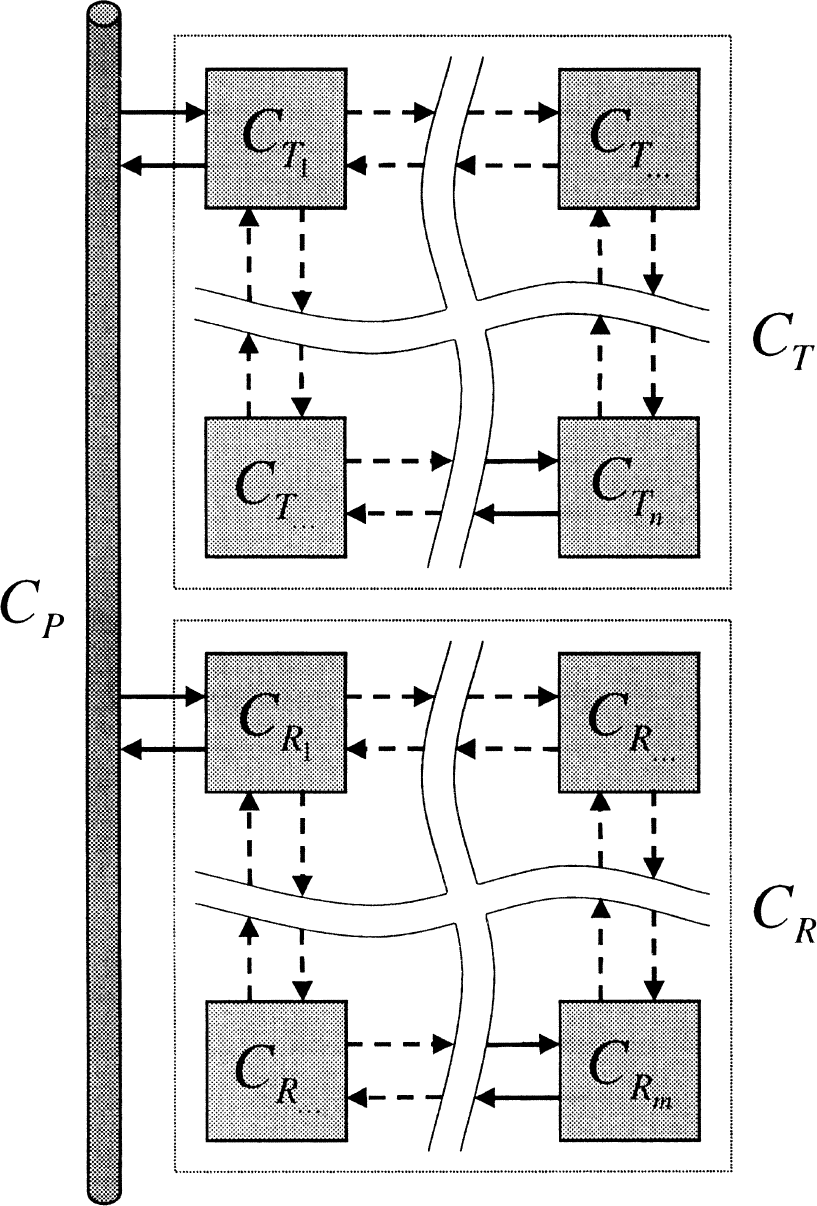
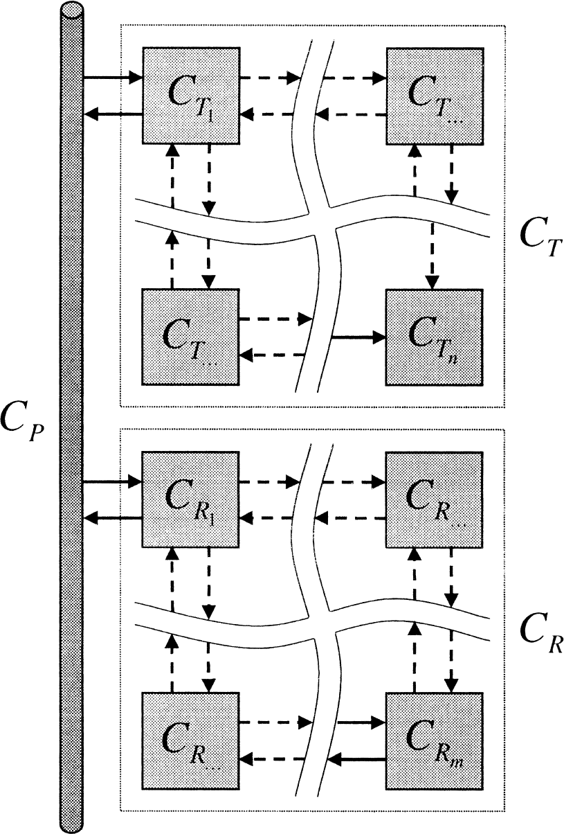
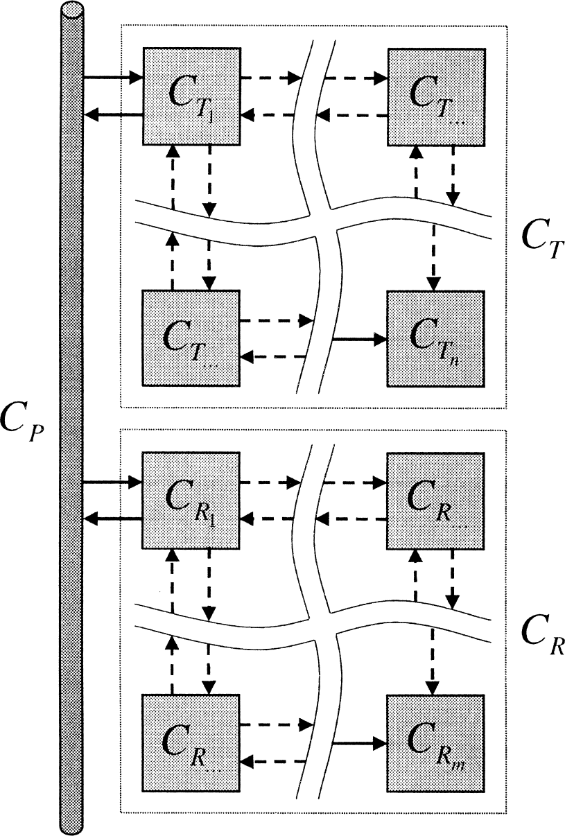
Consider a general PET reference compartmental system, as illustrated in Fig. 4, in which the measured radioactivity data consists of the total tissue concentration, CT, and the total reference tissue concentration, CR. The general PET reference tissue model restricts the interaction of the target and reference tissues solely through the plasma.
Generalized reference tissue model.
Its state space formulation is given by,
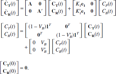
where the primes (′) refer to the reference tissue parameters. Often when a reference tissue model is used there is no associated measurement of the blood radioactivity concentration and so correction for blood contribution to the tissue signals is not possible. Here, the cases in which the blood activity does and does not contribute to the tissue signals are considered separately.
No blood volume
Consider the case in which there is no contribution of blood activity to the reference and target tissue signals (VB =V′B = 0).
Definition 2
Consider the set of linear compartmental reference systems (described by Eq. 3.1) where the connection of the reference tissue (m compartments) and the target tissue (n compartments) is solely through the plasma and the blood volume components are zero,
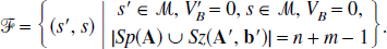
The set of reversible reference, reversible target models (Fig. 5) is defined as,

Reference tissue model with reversible target and reference tissues.
The set of reversible reference, irreversible target models (Fig. 6) is defined as,

Reference tissue model with irreversible target tissue and reversible reference tissue.
The set of irreversible references, irreversible target models (Fig. 7) is defined as,

Reference tissue model with irreversible target and reference tissues (single trap in each).
Theorem 2
A model s εF has a solution given by,

where
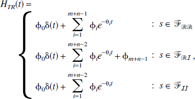
θ
i
> 0 and
If s εFRR,
If s εFRI,
If s εFII,
Again, it is straightforward to derive an indistinguishability and identifiability corollary directly from Theorem 2.
Corollary 2.1
Indistinguishability: any two reference tissue input models within the subset FRR (or similarly for FRI and FII) with a total of N tissue compartments (reference + target) are indistinguishable.
Corollary 2.2
Identifiability: the macro parameters (RI, VD/V′D or KI/V′D or KI/K′I) are uniquely identifiable from perfect input–output data.
Blood volume
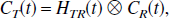
Now consider the general PET reference tissue model (Fig. 4) with blood volume in both the reference and target tissues (VB > 0, V′B > 0). The subsequent Theorem requires characterization of the tracer's behavior in blood and uses a result derived in Appendix A (Lemma 1).
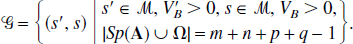
Definition 3
Consider the set of linear compartmental reference systems (described by Eq. 3.1) where the connection of the reference tissue (m compartments) and the target tissue (n compartments) is solely through the plasma, a whole blood volume components is present in each tissue and the tracer behavior in blood is described by Lemma 1 (Appendix B),
The set of reversible reference, reversible target models (Fig. 5) is defined as,

The set of reversible reference, irreversible target models (Fig. 6) is defined as,

The set of irreversible reference, irreversible target models (Fig. 7) is defined as,

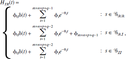
Theorem 3
A model s εG has a solution given by,
where
θ
i
≥ 0 and
If s εGRR,
If s εGRI,
If s εGII,
DISCUSSION
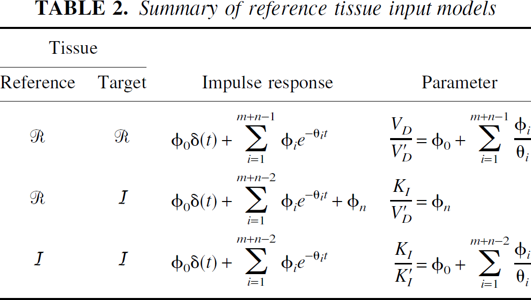
The current article is concerned with generic compartmental modeling of dynamic PET data, where the measured signal is the sum of all the constituent tissue compartments. General results have been derived for plasma input and reference tissue input models and are summarized in Tables 1 and 2. In each case, the tissue impulse response function is composed of a sum of exponentials, with an additional delta function term for reference tissue input models. There are three fundamental characteristics of the tissue impulse response function that are of interest: the initial value (which is equal to the value at t = 0), the step response (which is equal to the area under the impulse response function from t = 0 to t = ∞), and the steady state response (which is equal to the final value of the impulse response function). It can be seen that the macro parameters of the system (VD, KI, VD/V′D, KI/V′D, KI/K′I, BP.f1, and BP.f2) are simply related to these characteristics of the impulse response function independent of the number and topology of compartments. Furthermore, these macro parameters are uniquely identifiable from perfect input–output data.
Summary of plasma input models
Summary of reference tissue input models
Plasma input models
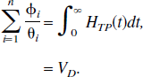
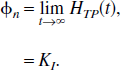
Plasma input models in PET often are treated as a gold standard (Kety, 1951; Sokoloff et al., 1977; Phelps et al., 1979; Mintun et al., 1984). The impulse response function is a sum of exponentials (Theorem 1), with the rate of delivery from the plasma, K1, given by the initial value of the impulse response function. For reversible tissue kinetics, the total volume of distribution, VD, is given by the integral of the impulse response function. For irreversible tissue kinetics, the irreversible uptake rate constant from plasma, KI, is given by the final value of the impulse response function. It may be noted that the final value of the impulse response function is equal to the limiting slope of a Patlak plot (Patlak et al., 1983). This result, as with the Patlak analysis, is independent of the number of intermediate reversible tissue compartments.
Reference tissue input models
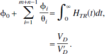
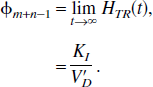
Reference tissue models have the advantage that no blood measurements are required and parameters are derived purely from the tomographic tissue data. For reference tissue input models, the general form of the impulse response function is a sum of exponentials plus a delta function term (Theorem 2). First, consider the results when there is no significant blood volume contribution to either the target or reference tissue. The coefficient of the delta function is equal to the relative delivery of tracer to the target versus the reference tissue, RI. For reversible kinetics in both the reference and the target tissues, the integral of the impulse response function is equal to VD/V′D. The relationship of this parameter to BP.f2 is discussed later. If the target tissue is irreversible and the reference tissue is reversible, the normalized irreversible uptake rate constant from plasma, KI/V′D, is given by the final value of the impulse response function. Again this is analogous to the reference tissue Patlak approach (Patlak and Blasberg, 1985). If both the target and reference tissues are irreversible, the ratio of the uptake rate constants between the target and reference, KI/K′I, is given by the integral of the impulse response function.
It is interesting to note the similarities and equivalences between reference tissue input models and plasma input models. In particular, for reversible kinetics the integral of the impulse response function for plasma input models is the volume of distribution, VD, and for reference tissue input models it is the relative volume of distribution, VD/V′D. Other similar analogies apply for the irreversible cases.
Model indistinguishability
As a consequence of Theorem 2, it can be shown that the topology of the compartments in the reference and target tissues is not important with regards to the macro parameters; it is merely the total number of compartments in the reference and target tissues that defines the set of indistinguishable reference tissue inputs models (Corollary 2.1).
Inclusion of blood volume
The current article also considers the case in which a significant contribution to the tissue signals is derived from the blood. If this is the case, a bias may be introduced in the macro parameter estimates. The magnitude of this bias is dependent on the blood volume, VB, the volume of distribution of the reference tissue, V′D, and the steady-state parent plasma-to-whole blood ratio, PB (Theorem 3). Similarly, a bias in the macro parameters for plasma input models, when blood contribution is ignored, can also be derived (results not shown). Investigators should be aware of these factors when applying plasma and reference input compartmental models or graphical methods such as the Patlak (Patlak et al., 1983) and Logan (Logan et al., 1990) plots without correcting for blood volume.
Radioligand binding studies
Now consider these models in the context of radioligand binding studies. There are several compartmental models in common use for the analysis of radioligand binding (Appendix C). The point of this appendix is to illustrate the relation between these commonly used compartmental models and the general results derived in the current article. The models in the appendix are formulated in terms of micro parameters, that is, individual rate constants for the exchange of tracer between compartments. In particular, they show that for reversible reference tissue models the integral of the impulse response function is simply related to binding potential in the same way in all cases.
Binding potential (BP) is a useful measure to quantify ligand–receptor interaction. The original definition of binding potential was introduced by Mintun et al. (1984) as the ratio of Bmax (the maximum concentration of available receptor sites) to the apparent KD of the free radioligand. To determine this parameter the free fractions of the radioligand in plasma (f1) and tissue (f2) need to be taken into account (Koeppe et al., 1991). It is necessary to distinguish between estimates of BP, BP.f1 and BP.f2. A summary of these parameters and their relation to the volumes of distribution is given in Table 3.
Summary of different binding potential measures
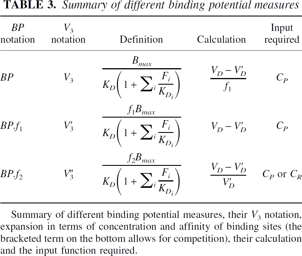
Summary of different binding potential measures, their V3 notation, expansion in terms of concentration and affinity of binding sites (the bracketed term on the bottom allows for competition), their calculation and the input function required.
BP.f2 may be determined from micro or macro parameters; either directly from the ratio of the micro parameters (typically k3 and k4), or indirectly from a volume of distribution ratio. The direct estimation is often susceptible to noise and the BP.f2 estimate may be unreliable. The second case requires a suitable reference region devoid of specific binding and requires that V′DF +V′DNS =VDF +VDNS (this assumption may be assessed by separate blocking studies). The determination of BP.f1 requires the same two assumptions, and is derived by subtracting the reference tissue volume of distribution from that of the target tissue. To derive the true binding potential, BP, the additional measure of the plasma free fraction is required, f1. The measurement of f1 may be determined from analysis of a blood sample, although these measurements often are inaccurate (Laruelle, 2000). These results are summarized in Table 3.
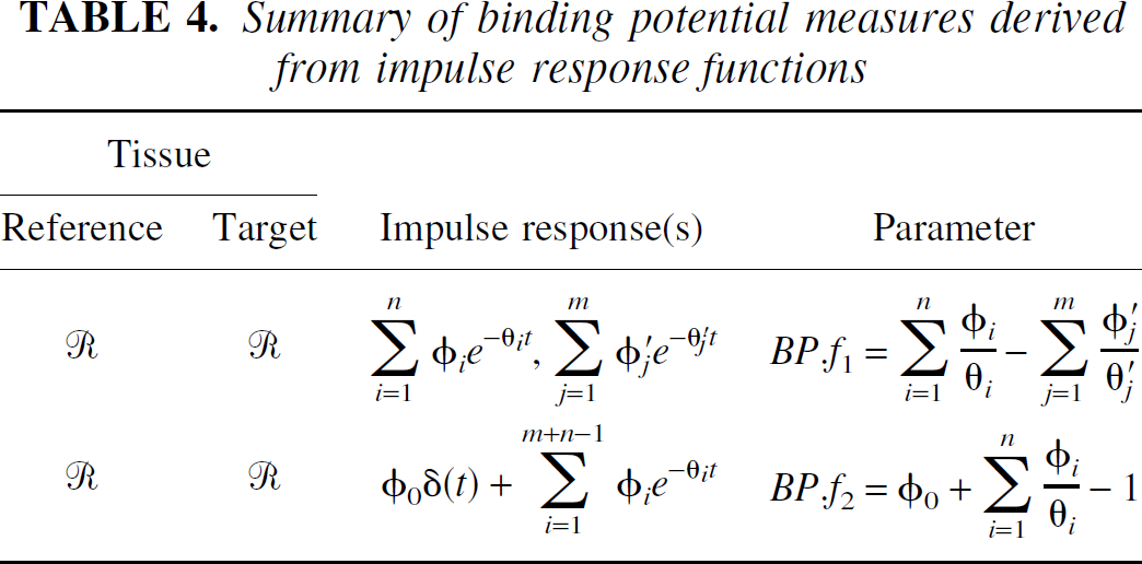
The estimation of these parameters for reversible reference tissue approaches with respect to radioligand binding are summarized in Table 4.
Summary of binding potential measures derived from impulse response functions
Particular compartmental structures
The reference tissue input model began as a 5-parameter model, the individual deliveries being unidentifiable without a plasma input function, leading to a reparameterization of the original 6-parameter system. This representation introduces a parameter for the ratio of influxes (or relative delivery) as RI (or R1) =K1/ K′1 (Blomqvist et al., 1989; Cunningham et al., 1991). With the assumption of equal blood–brain barrier transport rate constant ratios the model reduces to a 4-parameter system (Cunningham et al., 1991). The simplified reference tissue model assumes rapid exchange between the free and nonspecific compartments and has three parameters (Lammertsma and Hume, 1996). Finally, the Watabe reference tissue model returns to a 5-parameter formulation (Watabe et al., 2000). These models are summarized in Appendix C.
Model indistinguishability
To address the issue of the bias in the simplified reference tissue model for some tracers, Watabe et al. (2000) proposed a model with two tissues in the reference region. The theory presented in this article (Corollary 2.1) proves that the ‘Watabe’ reference tissue model is indistinguishable from the original reference tissue model (with five parameters) and will give the same value for the BP.f2. (Note: the ‘Watabe’ model may behave slightly different if the rate constants, k5 and k6, are fitted from a range of data initially (Watabe et al., 2000).
Reference tissue model bias
Recently, there has been some discussion about the biases that may be introduced by using the simplified reference tissue model (Parsey et al., 2000; Alpert et al., 2000; Gunn et al., 2000; Slifstein et al., 2000). A bias may be introduced for reference tissue input models in two ways: either from blood volume contribution to the tissue signals or from the use of a reduced order model. Theorem 3 summarizes the blood volume-induced biases for reference tissue input models. An expression for the blood volume-induced bias in reversible reference tissue input models, in the estimated
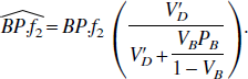
This general result shows that the bias is linear and allows the assessment of blood volume-induced biases for individual radioligands. Table 5 presents these results for [11C]raclopride where the parameter values are obtained from the literature (Lammertsma et al., 1996), except for the theoretical bias which is calculated as the bracketed term in Eq. 4.1. The reciprocal of PB was approximated by the plasma-to-blood ratio multiplied by the parent fraction for data at the end of the scanning period, although PB could be obtained from a fit using a model outlined in Appendix A. Good agreement is observed between the experimentally and theoretically derived biases.
Bias introduced by blood signal in BP.f2 for reversible reference tissue input model analysis
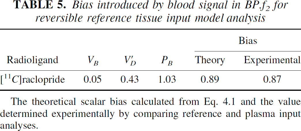
The theoretical scalar bias calculated from Eq. 4.1 and the value determined experimentally by comparing reference and plasma input analyses.
Irreversible systems
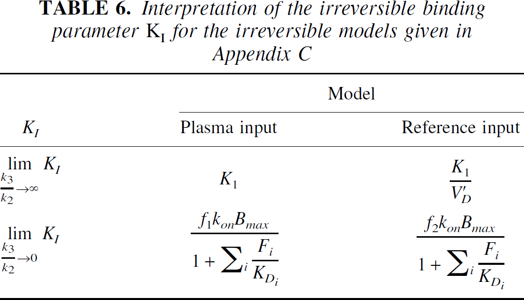
Dynamic radioligand PET data may exhibit irreversible characteristics when the time scale of the experiment is too short to fully characterize the (slow) reversible binding of the radioligand. Typically, longer scanning periods are impractical either because of discomfort to the subject or degradation of signal. In these situations one is restricted to parameters that represent irreversible kinetics, usually the k3 (micro parameter) or the KI (macro parameter). Whilst the k3 is often numerically unidentifiable, the KI does not suffer from this problem. However, the interpretation of the KI parameter is often confounded by blood flow (Table 6). Ultimately, with KI there is always an unfortunate trade off between the specificity and the magnitude of the signal—that is, when there is a large signal the parameter reflects blood flow and when the parameter reflects binding the signal is small.
Interpretation of the irreversible binding parameter KI for the irreversible models given in Appendix C
Blood and metabolism models
The current article has presented a generic model for metabolism and partitioning of parent tracer between plasma and red cells. This leads to a general form for a parent input function in terms of the whole blood curve. This functional form would allow general fitting of this function to discrete blood and metabolite measures. As such this would provide a flexible kinetic model for generating plasma parent input functions rather than using arbitrary functional forms. A particular example is presented in Appendix C. A general approach to modeling tracer metabolism has been presented previously by Huang et al. (1991), where they consider micro parameter formulations rather than considering the general form for the impulse response function. Particular compartmental structures also have been used to describe the metabolism of the parent tracer (Lammertsma et al, 1993; Gunn, 1996; Carson et al., 1997).
Summary
The current article has presented general theory for PET compartmental models, which shows that the required macro system parameters can be determined simply from the associated impulse response functions. The form of the relations between the macro parameters and the impulse response function are common to all models independent of the number and topology of compartments. Choosing a particular compartmental structure with a predefined number of compartments is equivalent to choosing the number of terms in the impulse response function. Ultimately, the number of numerically identifiable components in the impulse response function that can be determined from measured PET data will depend on both the statistical noise and the experimental design. The selection of a particular compartmental structure can meet with problems either if the number of identifiable components is less than the chosen model (for example, high noise) or more than the chosen model (for example, heterogeneity). The current article shows that a more general approach is possible where the macro parameters could be estimated by determination of the systems impulse response function without the need for a priori model selection. Approaches to the fitting of PET data to these generic models are being developed.
Footnotes
Acknowledgments:
The authors thank Federico Turkheimer and John Aston for useful discussions and comments on the manuscript.
1
This set includes all noncyclic systems and the subset of cyclic systems in which the product of rate constants is the same regardless of directions for every cycle (Goldberg, 1956; Godfrey, 1983).
2
Without loss of generality the nth compartment is defined to be the trap.
APPENDIX A
APPENDIX B
APPENDIX C
APPENDIX D
Glossary
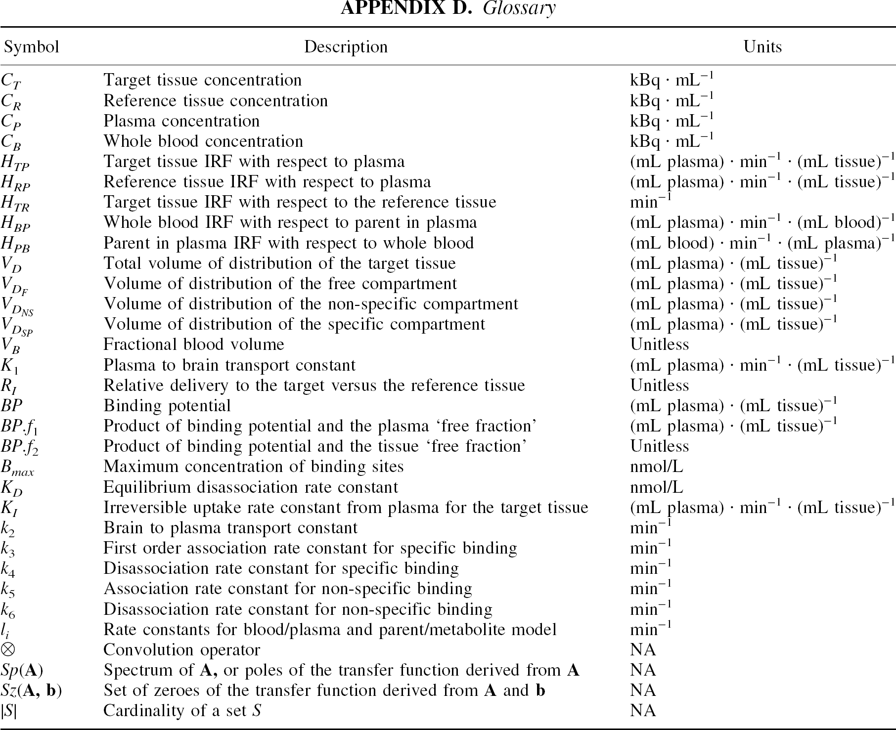
| Symbol | Description | Units |
|---|---|---|
| CT | Target tissue concentration | kBq · mL−1 |
| CR | Reference tissue concentration | kBq · mL−1 |
| Cp | Plasma concentration | kBq · mL−1 |
| CB | Whole blood concentration | kBq · mL−1 |
| HTP | Target tissue IRF with respect to plasma | (mL plasma)· min−1 · (mL tissue)−1 |
| HRP | Reference tissue IRF with respect to plasma | (mL plasma) · min−1 · (mL tissue)−1 |
| HTR | Target tissue IRF with respect to the reference tissue | min−1 |
| HBP | Whole blood IRF with respect to parent in plasma | (mL plasma)· min−1 · (mL blood)−1 |
| HPB | Parent in plasma IRF with respect to whole blood | (mL blood) · min−1 · (mL plasma)−1 |
| VD | Total volume of distribution of the target tissue | (mL plasma) ·(mL tissue)−1 |
| VDF | Volume of distribution of the free compartment | (mL plasma) · (mL tissue)−1 |
| VDNS | Volume of distribution of the non-specific compartment | (mL plasma) · (mL tissue)−1 |
| VDSP | Volume of distribution of the specific compartment | (mL plasma) · (mL tissue)−1 |
| VB | Fractional blood volume | Unitless |
| K 1 | Plasma to brain transport constant | (mL plasma) · min−1 · (mL tissue)−1 |
| RI | Relative delivery to the target versus the reference tissue | Unitless |
| BP | Binding potential | (mL plasma) · (mL tissue)−1 |
| BP.f 1 | Product of binding potential and the plasma ‘free fraction’ | (mL plasma) · (mL tissue)−1 |
| BP.f 2 | Product of binding potential and the tissue ‘free fraction’ | Unitless |
| Bmax | Maximum concentration of binding sites | nmol/L |
| KD | Equilibrium disassociation rate constant | nmol/L |
| KI | Irreversible uptake rate constant from plasma for the target tissue | (mL plasma) · min−1 · (mL tissue)−1 |
| K2 | Brain to plasma transport constant | min−1 |
| k 3 | First order association rate constant for specific binding | min−1 |
| k 4 | Disassociation rate constant for specific binding | min−1 |
| k 5 | Association rate constant for non-specific binding | min−1 |
| k 6 | Disassociation rate constant for non-specific binding | min−1 |
| li | Rate constants for blood/plasma and parent/metabolite model | min−1 |
| ⊗ | Convolution operator | NA |
| Sp( |
Spectrum of |
NA |
| Sz( |
Set of zeroes of the transfer function derived from |
NA |
| |S| | Cardinality of a set S | NA |