Sage Journals: Discover world-class research

Abstract

Cerebral blood flow can be measured with magnetic resonance imaging (MRI) by arterial spin labeling techniques, where magnetic labeling of flowing spins in arterial blood water functions as the endogenous tracer upon mixing with the unlabeled stationary spins of tissue water. The consequence is that the apparent longitudinal relaxation time (T1) of tissue water is attenuated. A modified functional MRI scheme for dynamic CBF measurement is proposed that depends on extraction of T1 weighting from the blood oxygenation level–dependent (BOLD) image contrast, because the functional MRI signal also has an intrinsic T1 weighting that can be altered by variations of the excitation flip angle. In the α-chloralose-anesthetized rat model at 7T, the authors show that the stimulation-induced BOLD signal change measured with two different flip angles can be combined to obtain a T1-weighted MRI signal, reflecting the magnitude of the CBF change, which can be deconvolved to obtain dynamic changes in CBF. The deconvolution of the T1-weighted MRI signal, which is a necessary step for accurate reflection of the dynamic changes in CBF, was made possible by a transfer function obtained from parallel laser-Doppler flowmetry experiments. For all stimulus durations (ranging from 4 to 32 seconds), the peak CBF response measured by MRI after the deconvolution was reached at 4.5 ± 1.0 seconds, which is in good agreement with (present and prior) laser-Doppler measurements. Because the low flip angle data can also provide dynamic changes of the conventional BOLD image contrast, this method can be used for simultaneous imaging of CBF and BOLD dynamics.

Keywords

Blood volume Energy Metabolism Neuronal activation Neuroimaging Oxygen

Abbreviations used: ASL, arterial spin labeling; BOLD, blood oxygenation level dependent; EPI, echo planar imaging; fMRI, functional magnetic resonance imaging; LDF, laser-Doppler flowmetry; MRI, magnetic resonance imaging; PET, positron emissions tomography; T1, apparent longitudinal relaxation time of tissue water; T2^*, apparent tissue water relaxation time of tissue water.

The early studies of Kety and Schmidt (1945) utilized nitrous oxide as tracers of diffusible inert gases to measure cerebral blood flow (CBF). Although these global methods were not sensitive enough to detect local CBF changes induced by peripheral sensory stimulation, these steady-state measurements provided the first quantitative window of tissue viability, metabolism, and function (for a review see Siesjo, 1978). Decades later, Sokoloff and coworkers (Reivich et al., 1969) introduced the idea of using intravascular radioactive tracers (e.g., [¹⁴C]iodoantipyrine) to measure regional CBF in absolute units at steady-state with an autoradiographic approach. To extend these autoradiograhic methods (which required the animal to be sacrificed) for human studies, analogous schemes were developed with positron emission tomography (PET) in conjunction with ¹⁵O-water in blood (Raichle et al., 1983), provided that water is a freely diffusible tracer that crosses the blood–brain barrier readily (Eichling et al., 1974). Although detection of ¹⁷O-water with magnetic resonance spectroscopy allowed CBF quantitation in a similar way, its low sensitivity did not allow significant improvements in spatial resolution (Arai et al., 1991; Pekar et al., 1991; Fiat and Kang, 1993). In the early 1990s, Kortesky and coworkers (Detre et al., 1992; Williams et al., 1992; Zhang et al., 1992) showed that the passage of water, which if assumed to be a freely diffusible tracer across the blood–brain barrier (Herscovitch et al., 1983), could be followed from changes in the intensity of the magnetic resonance imaging (MRI) signal arising from spins in the tissue water. As a consequence of both theoretical and experimental advances in functional MRI (fMRI) over the last decade, steady-state CBF measurements in absolute units can now be routinely achieved with high-spatial-resolution MRI utilizing water as an endogenous tracer (for reviews see Barbier et al., 2001a and Calamante et al., 1999).

Recently, however, there has been great interest in imaging CBF with high temporal resolution (Ogawa et al., 1998; Ugürbil et al., 2000) because the BOLD signal can be dynamically imaged in fMRI experiments, as shown from the very earliest days of fMRI (Blamire et al., 1992) and what is now called event-related fMRI (Buckner et al., 1996; Rosen et al., 1998). Relative changes in blood flow can be dynamically measured with laser-Doppler methods (Adachi et al., 1992; Koketsu et al., 1992; Underwood et al., 1992). Because the LDF signal is sensitive to the flux of red blood cells within the cerebral microvasculature, this technique is regarded as a standard for providing dynamic CBF measurements (Wadhwani and Rapoport, 1988). However, the laser-Doppler flowmetry (LDF) technique is rather invasive and has crude spatial resolution. In contrast, both the PET and MRI steady-state methods can potentially be modified for dynamic CBF mapping in a noninvasive manner. Although improving the PET method toward dynamic CBF mapping is limited by hardware (Raichle, 1987), modification of the MRI method is perhaps more feasible with current technology (Alsop and Detre, 1996).

Perfusion sensitivity in MRI is mainly achieved by variations of the arterial spin labeling (ASL) technique (for reviews see Barbier et al., 2001a and Calamante et al., 1999). Magnetic labeling of flowing spins in blood water (e.g., by inversion or saturation) functions as an endogenous tracer. Upon crossing the blood–brain barrier, the labeled spins mix with the unlabeled stationary spins of tissue water and as a consequence of which the apparent longitudinal relaxation time (T1) of tissue water is attenuated. Because the underlying assumption is that water is a freely diffusible tracer between blood and tissue compartments, increasing the temporal resolution while maintaining high sensitivity for CBF quantitation is a compromise between times required for spin labeling and relaxation. Although the ASL techniques suffer from poor temporal resolution because of the waiting period required for exchange of labeled and unlabeled spins, alternative labeling methods (e.g., dynamic or pseudocontinuous) can be used to improve the temporal resolution at the cost of CBF sensitivity (Schwarzbauer and Heinke, 1998; Silva and Kim, 1999; Barbier et al., 1999). Here we propose a customized fMRI scheme for dynamic CBF measurement that is dependent on extracting the T1 weighting from the BOLD signal. Although the gradient-echo BOLD image contrast with echo planar imaging (EPI) at high magnetic field strength shows high sensitivity toward apparent transverse relaxation time (T2^*) of tissue water (Ogawa et al., 1998; Ugürbil et al., 2000), there is also an intrinsic T1 weighting that can be altered by variations of the excitation flip angle (Gao et al., 1996; Glover et al., 1996). In the α-chloralose–anesthetized rat, we show that the stimulation-induced BOLD signal change measured with two different flip angles can be combined to obtain a T1-weighted MRI signal that reflects the magnitude of the CBF change. The dynamic changes in CBF can then be obtained by deconvolution of the T1-weighted MRI signal using a transfer function derived with respect to parallel LDF experiments. Details of this MRI method for dynamic CBF and BOLD imaging are discussed, where the simplicity and multimodal nature of the method demonstrate potential for physiologic and pathologic studies in rodent models.

THEORY

Spoiling the transverse magnetization (M_x) after the end of each EPI acquisition creates a new steady-state for the longitudinal magnetization (M_z) after n sequential excitations (Epstein et al., 1996; Gao et al., 1988; Spritzer et al., 1990)

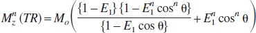
M_{z}^{n} (T R) = M_{o} (\frac{{1 - E_{1}} {1 - E_{1}^{n} {cos}^{n} θ}}{{1 - E_{1} cos θ}} + E_{1}^{n} {cos}^{n} θ)

(1)

where TR is the recycle time, θ is the flip angle, M_O is the initial longitudinal magnetization, E₁ = exp(–TR/T1), and T1 is the apparent longitudinal relaxation time (i.e., including the effects of CBF).

Equation 1 contains terms that represent parts of M_z at steady-state and the evolution from the fully relaxed condition to the steady-state. The dynamics of M_z evolution during rapid pulsing, equilibrating towards the steady-state, are dependent on TR, θ, and T1. If TR and θ are constant during this equilibration phase, then the T1 can be shown to be linked to CBF. Simulations using Bloch equations show that if a step change in CBF is introduced after this initial equilibration phase, M_z will establish another equilibration phase towards the different steady-state CBF value. Thus changes in T1 dynamically follow the different steady-state CBF values in both cases (because TR and θ are constant) because instantaneous changes in CBF cause slow variations in the T1-weighted MRI signal (i.e., the transfer function is limited by TR, θ, and T1). However the transition between the two steady-state CBF values can only be corrected by deconvolution (see below). For gradient echo imaging, M_x after the (n + 1)^th excitation is given by

M_{x}^{n + 1} (T E) = M_{z}^{n} (T R) \times (E_{2} sin θ)

(2)

where TE is the echo time and E₂ = exp(–TE/T2^*). Because the EPI signal (S) from a raw image (with flip angle of θ) is given by

S = \frac{1 - E_{1}}{1 - E_{1} cos θ} E_{2}

(3)

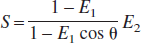
the BOLD signal change (ΔS/S) during a physiologic perturbation is given by

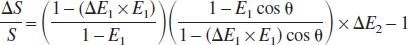
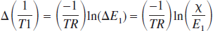
\frac{Δ S}{S} = (\frac{1 - (Δ E_{1} \times E_{1})}{1 - E_{1}}) (\frac{1 - E_{1} cos θ}{1 - (Δ E_{1} \times E_{1}) cos θ}) \times Δ E_{2} - 1

(4)

where ΔE₁ = exp[–TR ϗ Δ(1/T1)] and ΔE₂ = exp[–TE ϗ Δ(1/T2^*)]. The main requirement of this method is that the dynamic fMRI experiment be repeated twice with the same stimulation paradigm but with different flip angles: α and β are the low and high flip angles and represent the control (S_C) and labeled (S_L) signal intensities, respectively. Eq. 3 reduces to E₂ because the T1 contribution to the BOLD signal with a low flip angle of α is negligible (Gao et al., 1996; Glover et al., 1996), and thus Eq. 4 simplifies to exp[–TE × Δ(1/T2^*)] – 1, which is the traditional BOLD image contrast (Ogawa et al., 1998; Ugürbil et al., 2000). However, with a high flip angle of β, Eqs. 3 and 4 contain the T1 contributions to the BOLD signal. Because CBF depends on T1, the magnitude of the change in CBF (i.e., Δƒ) is due to an alteration of T1; i.e., Δ(1/T1) (see Appendix).

Δ f = λ \times Δ (\frac{1}{T 1})

(5)

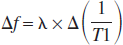
where Λ is the brain–blood partition coefficient for water (Roberts et al., 1996; Silva et al., 1997) and Δ(1/T1) reflects the change in CBF measured by ASL techniques (Barbier et al., 2001a; Calamante et al., 1999). Although theory (Detre et al., 1992; Williams et al., 1992; Zhang et al., 1992) suggests that Eq. 5 is valid for estimating the magnitude of the CBF changes with short TR, the deconvolution of the resulting T1-weighted MRI signal is needed to obtain the dynamics of the CBF changes (see above and below). The T1-weighted MRI signal is extracted from the dynamic fMRI data with the two flip angles (i.e., α and β).

Δ (\frac{1}{T 1}) = (\frac{- 1}{T R}) In (Δ E_{1}) = (\frac{- 1}{T R}) In (\frac{χ}{E_{1}})

(6)

where

\begin{matrix} χ = E_{1} \times Δ E_{1} = \frac{A - B}{A cos α - B cos β^{,}} A = \frac{1 + Δ S_{c} / S_{c}}{1 + Δ S_{L} / S_{L}^{,}} \\ B = \frac{1 - E_{1} cos α}{1 - E_{1} cos β^{.}} \end{matrix}

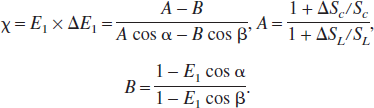
The main assumption in Eqs. 5 and 6 is that the changes in T2^* is identical in the two experiments and therefore can be canceled to reveal the T1-weighted MRI signal. It should be noted that the value of Δ(1/T1) will be the same for practically any arbitrary pair of α and β values, but that choice of the flip angle pair (where α < β) may affect perfusion sensitivity (see Appendix). Because the temporal profile of Δƒ can be modeled to be a convolution between a transfer function (i.e., h(t)) and the actual CBF dynamics as measured by LDF (i.e., Δƒ_LDF),

Δ f (t) = h (t) \otimes Δ f_{L D F} (t)

(7)

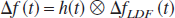
a temporal deconvolution is needed to obtain the actual CBF dynamics from MRI measurements [i.e., Δƒ(t)]. Because changes in T1 “follow” changes in CBF (from one steady-state to another), true transients or dynamics (in perfusion) can only be determined by a deconvolution of the MRI signal. Thus, the temporal resolution of the derived data is dependent on the accuracy of the deconvolution process. Simulations suggest that for MRI data with low signal-to-noise ratio, the accuracy of the deconvolution process becomes poor and the temporal resolution of CBF dynamics would be lower than the TR of the MRI data. Although in previous studies of dynamic CBF imaging the value of h(t) has been assumed (Silva and Kim, 1999), in this study h(t) was determined for each stimulus duration and the efficacy of a generalized h(t) for the somatosensory cortex for the rat was also examined.

MATERIALS AND METHODS

Animal preparation

Male Sprague-Dawley rats (250 ± 34 g; Charles River, Wilmington, MA, U.S.A.) were anesthetized with 1% to 2% halothane in a 70:30 mixture of N₂O and O₂ for surgical preparations. Intraperitoneal lines were inserted for administration of anesthetic and paralyzing agents. After tracheotomy was performed, rats were mechanically ventilated with 0.7% to 1.0% halothane in a 70:30 mixture of N₂O and O₂ and paralyzed with intraperitoneal injections of D-tubocurarine chloride (0.25 mg/kg per half hour). A femoral arterial cannula was inserted for continuous blood pressure monitoring and periodic sampling of blood gases (PO₂ and PCO₂) and pH.

A pair of needle electrodes was inserted underneath the skin of each forepaw. The forepaw stimulation (2 mA, 0.3 milliseconds, 3 Hz) was applied with different stimulus durations (4, 8, 16, and 32 seconds). Each stimulus duration was repeated at least twice (separated by at least 20 minutes), but more repetitions were used if the systemic physiological status of the subject was sustained for lengthy periods. All whiskers on the snout were cut to avoid spurious activations from the whisker region of somatosensory cortex, which is adjacent to the forelimb regions (Paxinos and Watson, 1997). The scalp was retracted and removed to reveal the skull around the bregma. After these surgical procedures, halothane anesthesia was discontinued and anesthesia was maintained with intraperitoneal injections of α-chloralose (initial 80 mg/kg, followed by 20 mg/kg per half hour). Before the start of MRI and LDF measurements, an approximately 1-hour period was allowed for clearance of halothane after switching to α-chloralose anesthesia. The physiologic variables were controlled within the normal range (pH = 7.38 ± 0.07, PCO₂ = 36.7 ± 4.8 mm Hg, PO₂ = 148 ± 18 mm Hg).

For the fMRI experiments (n = 10), the skull was cleaned of all tissues and a layer of Saran Wrap was placed over the exposed wound. The rat was placed in a custom-made rodent holder, which allowed the bregma to be positioned at the center of the radio frequency coil and the head could be fixed with bite-bars in a stereotaxic-like manner. The head was tightly fixed by foam cushions on either side of the head to minimize motion. The rat was covered with a temperature controlled water blanket to maintain body temperature (–37°C) throughout the experiments. The rat was then inserted into the magnet and the head was positioned at the magnet isocenter.

For the LDF experiments (n = 9), the rat was placed in a stereotaxic frame (David Kopf Instruments, Tujunga, CA, U.S.A.), which sat on a vibration-free table inside a Faraday cage. A temperature controlled water blanket was placed under the rat to maintain body temperature (–37 °C) throughout the experiments. The skull over the forelimb somatosensory cortex (4 mm lateral to the midline and 1 mm anterior) was thinned (Detre et al., 1998) and special care was taken not to expose the dura.

Functional MRI experiments

All fMRI data were acquired on a 7T AVANCE (Bruker Instruments, Billerica, MA, U.S.A.) horizontal-bore spectrometer, which is equipped with actively shielded shim/gradient coils (18 G/cm) operating at 300.3 MHz for ¹H. The transceiver system consisted of a ¹H resonator (8 cm) for transmission of radiofrequency pulses and an orthogonally oriented ¹H surface coil receiver (1 cm). The two magnetically isolated coils were positioned orthogonal relative to one another such that the homogeneous regions of the two coils coincided, which minimized sensitivity losses in the receiver coil and permitted localized shimming and homogeneous transmission, as is required for uniform spin labeling in ASL techniques (for reviews see Barbier et al., 2001a and Calamante et al., 1999). Perfusion sensitivity by ASL techniques can be obtained by both distal or “neck” (e.g., Barbier et al., 1999; Silva and Kim, 1999) and proximal or “head” (e.g., Kida et al., 2000; Schwarzbauer et al., 1996) spin labeling coils using the two-coil setup, where in the former case the labeling coil is located around the neck region and in the latter case the labeling coil is the homogenous transmitter. We chose the latter two-coil setup because of concerns of radiofrequency power deposition with the former two-coil setup, which can affect the temperature of the blood entering the brain (Barbier et al., 2001b).

High spatial resolution anatomical MRI data were acquired in the coronal plane (Kida et al., 2001) for positioning the slices over the somatosensory cortex. A thick coronal slice (~10 mm) was shimmed (<20 Hz) to improve the sensitivity for fMRI experiments. Single-shot gradient echo EPI data (for all fMRI experiments) were acquired with sequential sampling (Hyder et al., 1995) (data matrix = 32 × 32, in-plane resolution = 625 × 625 μm, slice thickness = 2 mm, TE = 20 milliseconds, TR = 500 milliseconds). For each stimulus condition, fMRI data were acquired with low (α = 19° ± 7°) and high (β = 59° ± 11°) flip angles. The absolute CBF under resting conditions was acquired with the conventional ASL technique using slice-selective and nonselective inversion recovery EPI data with multiple inversion recovery times (ranging from 100 to 2,000 milliseconds) as previously described for the current two-coil setup (e.g., Hyder et al., 2000; Kida et al., 2000) (slice thickness for excitation = 2 mm, slice thickness for inversion = 10 mm, data matrix = 32 × 32, in-plane resolution = 625 × 625 μm, TE = 20 milliseconds, TR = 8 seconds). An absolute CBF map was measured before and after each experimental fMRI run.

Laser-Doppler flowmetry experiments

All LDF data were acquired with a PF5000 (Perimed, Stockholm, Sweden) probe using a 780-nm-wavelength light source and operating at 250 milliseconds temporal resolution. Although the collected data were represented as percentage from the prestimulation baseline values, only the LDF temporal profile was needed (as in Eq. 7) for the current study. Because the transmission and detection probes were separated by 250 μm, we detected a small volume (approximately 1 mm³) in the cortex that coincided with the location of the largest BOLD activity detected by fMRI for this rat model (Kida et al., 2001).

Data analysis

All fMRI image analyses were performed using home-written software on MATLAB domain (MathWorks, Natick, MA, U.S.A.). All data sets were examined for movement artifacts by a center of mass analysis, which was restricted to voxels within the brain boundary (Yang et al., 1998). If the center of mass of a raw image in a series shifted by more than one quarter of a pixel (in either plane), the entire series was removed from analysis. The fMRI data with low (α) and high (β) flip angles were analyzed in the same manner to generate t and ΔS/S maps. These functional maps were created on a pixel-by-pixel basis using images in the prestimulation and the stimulation periods, because the poststimulation signal returned to baseline in a gradual manner (Kida et al., 2001). Because comparison of the phase and magnitude time series of the BOLD signal (data not shown) suggested that the fMRI activation map obtained from the low flip angle data (α) series (i.e., T2^* weighted) was devoid of large vessel artifacts (Menon, 2002), we used the functional map with low flip angle (α) to avoid the inclusion of inflow effects from large blood vessels in the CBF data.

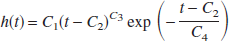
The fractional changes in CBF (i.e., Δƒ/ƒ) were calculated by combining Δƒ (from Eq. 5) with the absolute CBF measured by an ASL technique (see above). For each rat, time courses from the same three or four activated voxels within the somatosensory cortex were analyzed. For each stimulus duration, the time courses from all rats were averaged. A similar group averaging was also performed with the LDF data. For each stimulus duration, the transfer function in Eq. 7, h(t), was obtained by deconvolution of the CBF data obtained by MRI and LDF, which was defined by a gamma variate function

h (t) = C_{1} {(t - C_{2})}^{C 3} exp (- \frac{t - C_{2}}{C_{4}})

(8)

where C₁ – C₄ are constants that were analytically determined. A generalized transfer function for the somatosensory cortex was determined by averaging the h(t) obtained for all stimulus durations. Dynamics of Δƒ/ƒ for the deconvolved T1-weighted MRI signals and LDF signals were compared to determine the efficacy of the generalized h(t). Although the error analysis for the LDF data was based on the standard deviation (SD) from all combined measurements, the error analysis for the MRI data was determined by propagation of SD from the different MRI measurements (see Appendix). Because typical rodent brain data from our 7T system have high signal-to-noise ratio for TR ≥ 500 milliseconds (Kida et al., 2001; 2002), simulations suggest that the deconvolved MRI data do not suffer sufficient degrading and the temporal resolution of CBF dynamics (obtained from the deconvolution) is expected to approximate the TR of our data.

RESULTS

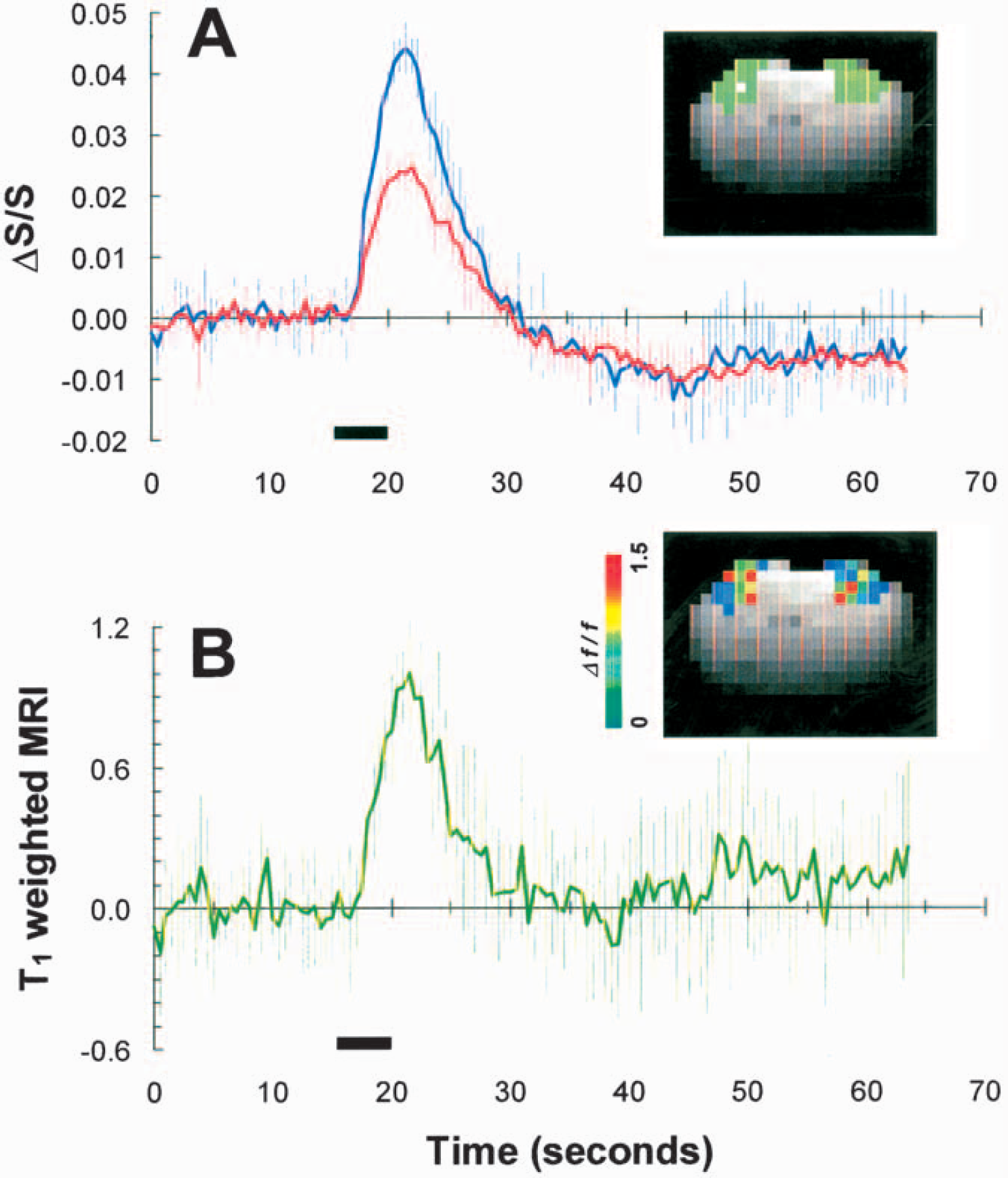
Figure 1A shows the representative time courses of BOLD signal change or ΔS/S (average of four trials) during 4-second forepaw stimulation with two different flip angles (20° and 60°) from a single voxel indicted in the inset (white square), which shows the BOLD functional map obtained with the low flip angle data. The time-to-peak of the ΔS/S time courses was not significantly dependent on the flip angle (~6 seconds). The relative difference between the peak amplitudes of the ΔS/S time courses with the different flip angles (i.e., 2.2% ± 0.5% and 1.3% ± 0.5% averaged from β ranging from 48° to 73° (i.e., 59° ± 11°) and α ranging from 10° to 28° (i.e., 19 ± 7°) for all rats) indicates the varied weighting of the first and second products on the right hand side of Eq. 4 which allowed extraction of the CBF change (see Appendix) using Eq. 6. Figure 1B shows the time course of the T1-weighted MRI signal obtained from the data shown in Fig. 1A (for an individual subject) with α = 20° and β = 60°, where the corresponding Δƒ/ƒ map is shown as an inset. The time courses of the T1-weighted MRI signal obtained with different pairs of α and β values were insignificantly different (data not shown). However, the time courses of ΔS/S and the T1-weighted MRI signals were significantly dissimilar after stimulation offset: the BOLD signal had an undershoot whereas the CBF signal returned to baseline.

Figure 1B shows the time course of the T1-weighted MRI signal obtained from the data shown in Fig. 1A (for an individual subject) with α = 20° and β = 60°, where the corresponding Δƒ/ƒ map is shown as an inset. The time courses of the T1-weighted MRI signal obtained with different pairs of α and β values were insignificantly different (data not shown). However, the time courses of ΔS/S and the T1-weighted MRI signals were significantly dissimilar after stimulation offset: the BOLD signal had an undershoot whereas the CBF signal returned to baseline.

Fig. 1.

(A) Time courses of ΔS/S with two different flip angles (blue (ß) = 60° and red (α) = 20°) during 4 seconds of forepaw stimulation in the α-chloralose anesthetized rat. The relative difference between the peak amplitudes indicates the altered weighting of the first and second terms on the right-hand side of Eq. 4. Inset: BOLD activation map (with α only) of stimulation of both paws shown in a coronal slice, where the ΔS/S time courses are from the white square. (B) The CBF change can be extracted from the relative difference between the data sets in panel A by using Eq. 6, which results in the (predeconvolved) T1-weighted MRI signal. Inset: CBF change activation map of stimulation of both paws shown in a coronal slice. Black bar represents the stimulus duration.

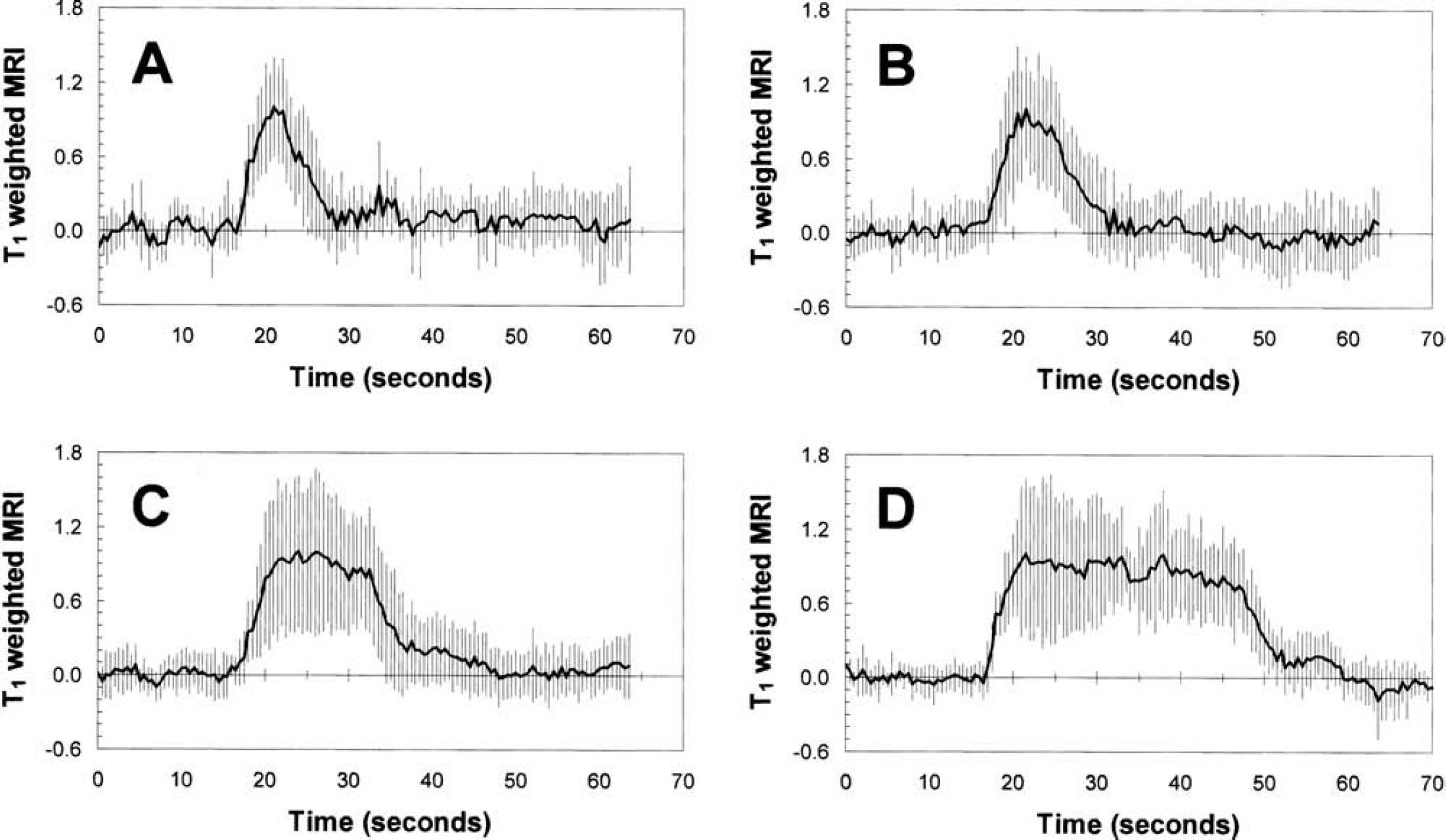
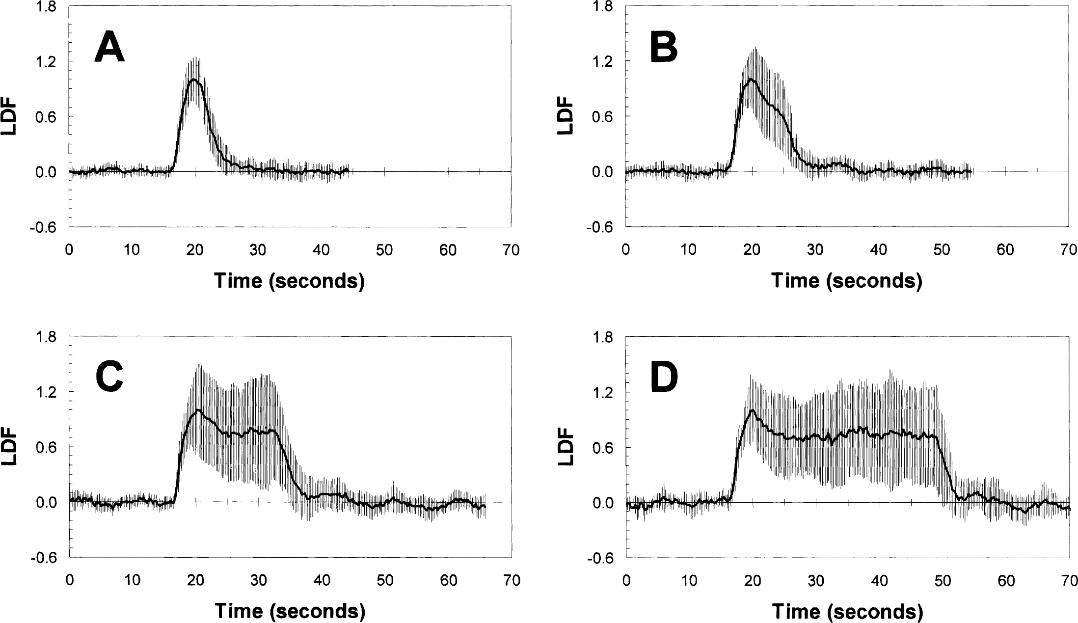
Figure 2 shows the time courses of T1-weighted MRI signals for all the different stimulus durations (4, 8, 16, and 32 seconds) averaged across all rats (n = 10). The time courses were obtained from approximately the same small region (three or four voxels) within the forelimb area (Paxinos and Watson, 1997) that overlapped with the volume detected by the LDF probe (Detre et al., 1998). The CBF value in this somatosensory region was 0.8 ± 0.1 mL·Dg⁻¹·Dmin⁻¹ under the current α-chloralose regimen. The value of Δƒ/ƒ for the 4-second stimulation was approximately 20% lower than the values obtained for the longer stimulus durations. The magnitudes of the CBF change measured by MRI for the longer stimulus durations were in agreement with prior results for the same model (Silva et al., 1999; Hyder et al., 2000). The time-to-peak for the T1-weighted MRI signals time courses ranged from about 5.5 seconds to 7.0 seconds. To deconvolute the T1-weighted MRI signal time courses, as shown in Eq. 7, we performed CBF measurements with an LDF probe under the same stimulus and physiologic condition used in the fMRI experiments. The observed area of LDF measurements was approximately 1 mm deep from the dura with a volume of approximately 1 mm³ using a 780-nm-wavelength light source and a 250 μm separation between transmission and detection probes (Nielsen and Lauritzen, 2001). In comparison, the MRI-sensitive area analyzed for the deconvolution was 1.1 ± 0.4 mm³. Figure 3 shows the LDF time courses obtained for all different stimulus durations (4, 8, 16, and 32 seconds) averaged across all rats (n = 10). The LDF time courses for the longer stimulus durations (16 and 32 seconds) showed a peak followed by a plateau during the stimulation period, whereas the shorter stimulus durations (4 and 8 seconds) showed only a peak. The time-to-peak for the LDF time courses (3.9 ± 1.0 seconds) was much faster than the time-to-peak for the (predeconvolved) T1-weighted MRI signals time courses (6.4 ± 1.9 seconds). Similar LDF temporal profiles have been reported previously for the same model (Ances et al., 2000; Matsuura and Kanno, 1999).

Fig. 2.

The (predeconvolved) T1-weighted MRI signal time courses for 4-second (A), 8-second (B), 16-second (C), and 32-second (D) stimulation durations averaged across all rats (n = 10), where the vertical lines indicate the SD. The time courses were obtained from approximately the same small region (1.1 ± 0.4 mm³) within the forelimb area and the time-to-peak for the (predeconvolved) T1-weighted MRI signal time courses was 6.4 ± 1.9 seconds (stimulus onset at 16 seconds).

Fig. 3.

The LDF signal time courses for 4-second (A), 8-second (B), 16-second (C), and 32-second (D) stimulation durations averaged across all rats (n = 10), where the vertical lines indicate the SD. The time courses were obtained from approximately the same small region (~1 mm³) within the forelimb area and the time-to-peak for the LDF signal time courses was 3.9 ± 1.0 seconds (stimulus onset at 16 seconds).

For each stimulus duration, a transfer function [i.e., h(t)] was calculated with the data shown in Figs. 2 and 3 using Eq. 7. Although the individual transfer function for the respective stimulus duration can be easily applied to deconvolute the T1-weighted MRI signals for that stimulus duration, we tested the efficacy of using arbitrarily chosen transfer functions (determined for any stimulus duration) to deconvolute the T1-weighted MRI signals. In Fig. 4, the deconvolved T1-weighted MRI signals are shown, where the different stimulus durations are shown in rows and the different transfer functions (as determined for the respective stimulus durations) are shown in columns. The data shown in the diagonal of Fig. 4 indicate the deconvolved T1-weighted MRI signals using the “exact” transfer function determined for the respective stimulus duration, whereas the data shown in off-diagonal regions are the deconvolved T1-weighted MRI signals using “arbitrary” transfer functions. The excellent deconvolution of the MRI time courses with “exact” or “arbitrary” transfer functions suggests that a generalized transfer function (with values of C₁ – C₄ of −1.07 ± 0.09, 0.50 ± 0.01, 1.00 ± 0.01, and 0.53 ± 0.03 in Eq. 8) can be used with good experimental accuracy. The time-to-peak for the deconvolved T1-weighted MRI signals using the generalized transfer function (4.5 ± 1.0 seconds) was not significantly different from the time-to-peak for the LDF time courses (3.9 ± 1.0 seconds). The excellent agreement between the time-to-peak of the deconvolved T1-weighted MRI signals (gray line) and LDF signals (black line) time courses, shown in Fig. 5, suggests that the output of the transfer function retained the temporal resolution of the MRI data. In each case, the deconvolved T1-weighted MRI signal (reflecting dynamics of the corrected CBF signal; gray line) is significantly different and separated from the pre-deconvolved T1-weighted MRI signal (reflecting dynamics of the noncorrected CBF signal; dotted line).

DISCUSSION

Most ASL techniques suffer from poor temporal resolution because of the waiting period required for the exchange of labeled arterial spins with unlabeled tissue spins. Dynamic or pseudocontinuous spin labeling schemes can be used to improve the temporal resolution, but this is achieved at the cost of CBF sensitivity because of the decreased times used for spin labeling and relaxation (Barbier et al., 1999; Schwarzbauer and Heinke, 1998; Silva and Kim, 1999). Because ASL methods inherently have low signal-to-noise ratio (Alsop and Detre, 1996; Calamante et al., 1999; Zhou and van Zijl, 1999), sacrificing further sensitivity may limit quantifying CBF changes in functional imaging studies. Because there is an intrinsic T1 weighting in the BOLD signal (Eq. 3), the combination of stimulation-induced ΔS/S values measured with different flip angles (Fig. 1) illustrates a T1-weighted MRI signal that reflects the magnitude of the CBF change (Fig. 2). Because LDF experiments measure the real CBF dynamics (Fig. 3), a transfer function (Eq. 8) can be used to deconvolute the T1-weighted MRI signal (Fig. 2) to reflect dynamic changes in CBF (Figs. 4 and 5). Although the temporal resolution in the current study was 500 milliseconds, higher temporal resolution data can be used without significant sensitivity losses for dynamic CBF measurements. Because the transfer functions generated for each stimulus duration were insignificantly different in deconvoluting the T1-weighted MRI signals for the different stimulus durations (Fig. 4), a generalized transfer function (see Results) can be used for CBF dynamics with this MRI approach (Fig. 5). Although it is possible that the time course of the predeconvolved T1-weighted MRI signal may be related to vascular space occupancy, a recent blood volume method that exploits the small T1 differences between blood and tissue water (Lu et al., 2003), the time course of the deconvolved T1-weighted MRI signal has been “corrected” for dynamics in CBF.

Fig. 4.

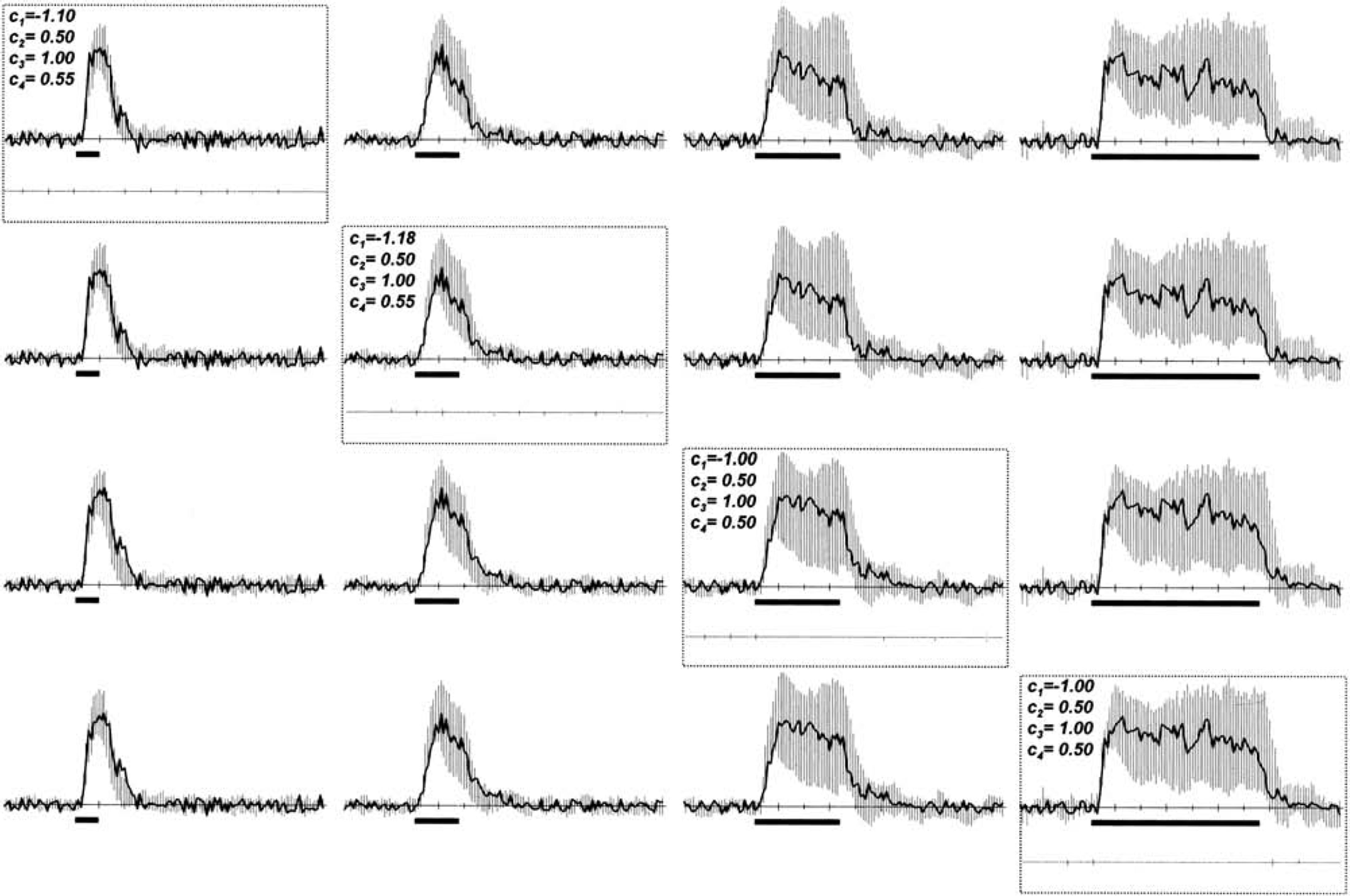
The deconvolved T1-weighted MRI signal time courses are shown for different stimulus durations (in rows) using different transfer functions (in columns). The data shown in the diagonal (outlined with dotted rectangles) indicate the deconvolved T1-weighted MRI signal time courses using the “exact” transfer function determined for the respective stimulus duration, whereas the data shown in off-diagonal regions are the deconvolved T1-weighted MRI signal time courses using “arbitrary” transfer functions. The excellent deconvolution of the T1-weighted MRI signal time courses with “exact” or “arbitrary” transfer functions suggests that a generalized transfer function for the somatosensory cortex can be used with good experimental accuracy. The difference between the LDF and deconvolved T1-weighted MRI signals is shown in gray. The time-to-peak for the deconvolved T1-weighted MRI signal time courses using the generalized transfer function (i.e., with values of C₁ – C₄ of −1.07 ± 0.09, 0.50 ± 0.01, 1.00 ± 0.01, and 0.53 ± 0.03 in Eq. 8) was not significantly different from the time-to-peak for the LDF signal time courses (i.e., 4.5 ± 1.0 seconds vs. 3.9 ± 1.0 seconds).

Fig. 5.

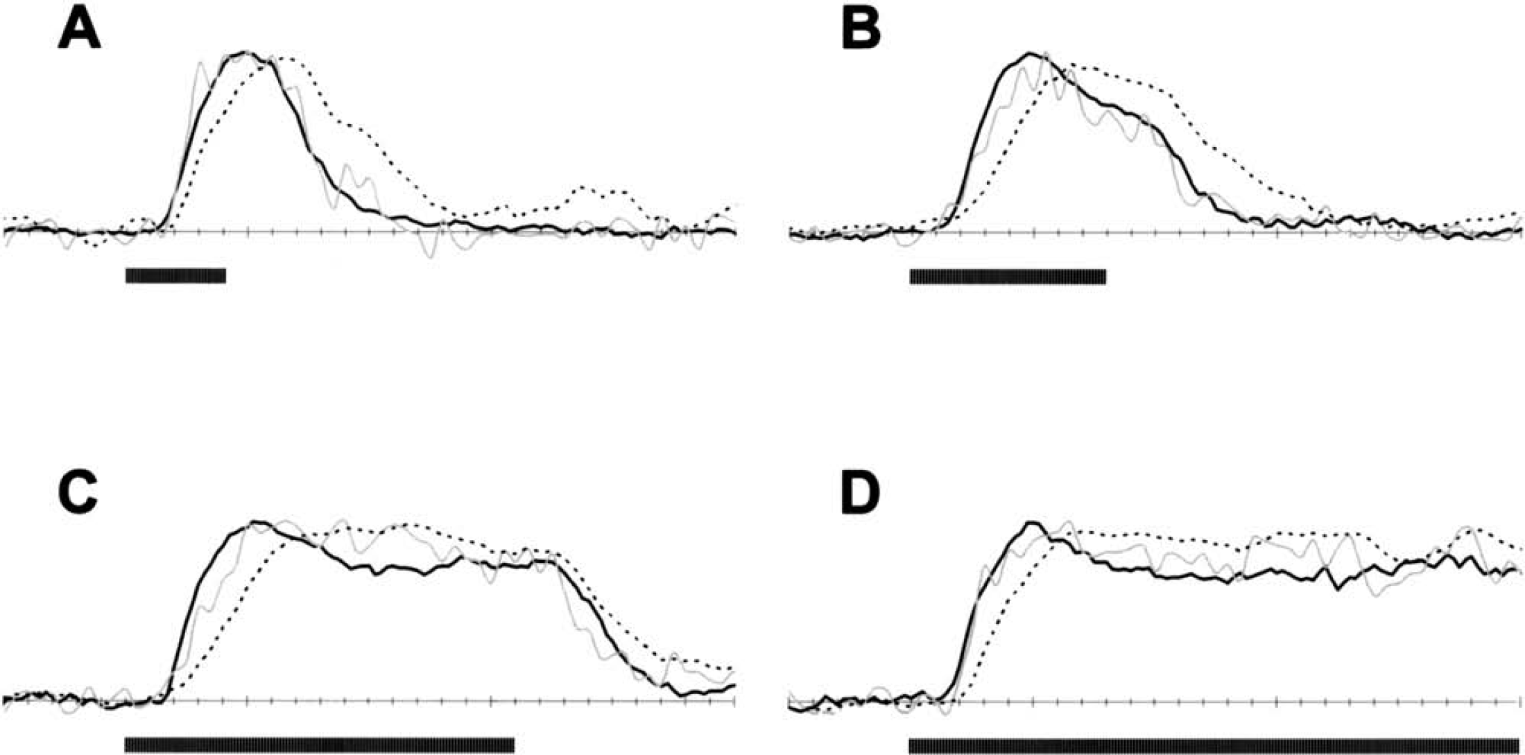
Comparison of fractional changes in the LDF signals (solid black line) and T1-weighted MRI signals, for both the deconvolved (solid gray line) and predeconvolved (dotted line) situations with 4-second (A), 8-second (B), 16-second (C), and 32-second (D) stimulation durations. In each case, the LDF signals changes are in good agreement with the time courses of the deconvolved T1-weighted MRI signals because these signals were “calibrated”—using the generalized transfer function for the somatosensory cortex as shown in Fig. 4—to reflect the measured CBF dynamics. In each case, time-to-peaks for the predeconvolved T1-weighted MRI signals (~6 seconds) were significantly delayed (by ~2 seconds) from the time-to-peaks for the deconvolved T1-weighted MRI signals (~4 seconds) or the LDF signals (~4 seconds). Each horizontal tick mark on the horizontal axis represents 1 second, and the horizontal bar represents the stimulus duration.

At low magnetic field strength, the inflow effect with conventional gradient echo or EPI pulse sequences is considered to be a nuisance (Duyn et al., 1994; Frahm et al., 1994) because the sensitivity of BOLD image contrast for small blood vessels is low (Ogawa et al., 1993; Kennan et al., 1994; Weisskoff et al., 1994), and therefore the inflow effect is sensitive to deoxyhemoglobin washout in large blood vessels. In contrast, at high magnetic field strength the sensitivity of BOLD image contrast for capillaries and venules is higher (Kennan et al., 1994; Ogawa et al., 1993; Weisskoff et al., 1994) and the inflow effect in large arteries and draining veins can be minimized by using a low flip angle and a slow repetition time (Ogawa et al., 1998; Ugürbil et al., 1998). However, only into the parenchyma will the enhanced signal from inflow be beneficial (Glover et al., 1996). The inflow effect in capillaries and venules is relatively small (Gao et al., 1996) because the flow of red blood cells is higher in large vessels than in small vessels (e.g., 7 to 10 cm/s versus 0.1 to 0.5 cm/s, respectively). Prior studies from diffusion-weighted spin echo fMRI of the same rodent model (Hyder, 2004; Lee et al., 1999) suggest that at high fields these types of inflow effects are less pronounced. However, gradient echo fMRI data may still partially be susceptible to some artifacts even at high fields. Our prior rodent studies on the same scanner with spin echo and gradient echo data (Hyder et al., 2000; Kida et al., 2000) suggest that choice of experimental parameters in gradient echo data (e.g., voxel size, slice thickness, echo time, flip angle, repetition time) can further minimize or help to identify the contaminating signals from large blood vessels. In addition to optimized experimental parameters in the current study (see Functional MRI experiments in Materials and Methods) based on our current findings for excluding nuisance signals from large blood vessels, the CBF data in the current study were analyzed specifically to mask out any activities from unwanted inflow effects for large vessels by the BOLD data with low flip angle, which we believe is devoid of large vessel artifacts based on a comparison of the phase and magnitude time series of the BOLD data (Menon, 2002) (see ‘Data analysis' in Materials and Methods).

The proposed MRI scheme for dynamic CBF measurements, by nature of its design, requires the assumption that two consecutive fMRI experimental runs (with low and high flip angles) are physiologically identical. The hemodynamic responses were reproducible for these consecutive experimental runs as reflected by the mean and standard deviation of the T1-weighted MRI signal data (Fig. 1). Another requirement of this MRI scheme is to separately measure absolute CBF under the resting condition, as measured by conventional ASL techniques, so that the fractional change in CBF can be calculated (Fig. 2). To ensure that the appropriate magnitude of CBF change was calculated, the absolute CBF data were collected before and after each fMRI experimental run (see Materials and Methods). In comparison, Silva and Kim (1999) have proposed a pseudocontinuous ASL method for dynamic CBF mapping where two experimental runs are also necessary (i.e., with and without spin tagging) and the combination provides absolute CBF data. However, this method uses the two-coil setup where the labeling coil is located around the neck region. There are some concerns of radiofrequency power deposition with this two-coil setup (Barbier et al., 2001b), which in turn can affect the temperature of the blood entering the brain (Trübel et al., 2003) and alter oxidative metabolism (CMR_O₂) at baseline (Hyder et al., 2001).

The “nominal” temporal resolutions of the Silva and Kim (1999) method and the current approach are ultimately dependent on the accuracy of the deconvolution process because the deconvolved signal has to accurately match the time course of the dynamics of the true changes in CBF. If a smoothed function of CBF dynamics is used to obtain the transfer function, then an apparently smoothed deconvolved signal will be generated and the method will have the same temporal resolution as the initial MRI measurements. In the Silva and Kim (1999) study the transfer function, needed to deconvolve the CBF data, was assumed for a single stimulus duration. In comparison, in the current study transfer functions were determined on the basis of parallel LDF and MRI measurements for several stimulus durations. Thus, it is plausible that the current method will have slightly lower temporal resolution but the generalized transfer function for the somatosensory cortex (Fig. 4) is likely to be more widely applicable because it is based on real CBF measurements. However, it is possible that there may be some misregistration of tissue volumes sampled by LDF and MRI. Although the LDF method measures red blood cell flow, it was assumed that the measurement is an accurate reflection of CBF dynamics because the temporal responses of red blood cells and plasma are not significantly different (Matsuura and Kanno, 1999).

Several studies have shown the estimation of changes in CMR_O₂ by using ASL methods combined with BOLD measurements in functional activation studies (Davis et al., 1998; Hoge et al., 1999; Hyder et al., 2001; Kim et al., 1999). Although MRI pulse sequence manipulations can allow the ASL contrast to be almost simultaneously implemented with the BOLD contrast, the combined CBF and BOLD measurements as shown here may be useful in future studies for detecting dynamics in CMR_O₂.

CONCLUSION

Dynamic changes in CBF were measured noninvasively with MRI without the need for ASL. Because the inflow signal from the parenchyma was specifically enhanced by this approach, fractional changes in CBF were quantitated with high sensitivity of BOLD data. Thus, this modified scheme for fMRI allows multimodal imaging of both CBF and BOLD dynamically. The deconvolution of the inflow signal from the parenchyma was made possible by a generalized transfer function for the somatosensory cortex (in the rat) derived with respect to parallel LDF experiments. Because of the simplicity and multimodal nature of this fMRI scheme, it is expected that this method may be used in future physiologic and pathologic rodent and human studies with high spatiotemporal resolution.

Footnotes

Acknowledgements

The authors thank engineers Terry Nixon, Peter Brown, and Scott McIntyre of the Magnetic Resonance Research Center at Yale for technical support and Drs. Fuqiang Xu, Maolin Qiu, Arien Smith, Kevin Behar, and Douglas Rothman for helpful discussions.

APPENDIX

References

Adachi

Baramidze

Sato

(1992) Stimulation of the nucleus basalis of Meynert increases cortical cerebral blood flow without influencing diameter of the pial artery in rats Neurosci Lett 143:173–176

Alsop

Detre

(1996) Reduced transit-time sensitivity in noninvasive magnetic resonance imaging of human cerebral blood flow J Cereb Blood Flow Metab 16:1236–1249

Ances

Greenberg

Detre

(2000) Effects of variations in interstimulus interval on activation-flow coupling response and somatosensory evoked potentials with forepaw stimulation in the rat J Cereb Blood Flow Metab 20:290–297

Arai

Mori

Nakao

Watanabe

Kito

Aoki

Mori

Morikawa

Inubushi

(1991) In vivo oxygen-17 nuclear magnetic resonance for the estimation of cerebral blood flow and oxygen consumption Biochem Biophys Res Commun 179:954–961

Barbier

Silva

Kim

Williams

Koretsky

(1999) Perfusion analysis using dynamic arterial spin labeling (DASL) Magn Reson Med 41:299–308

Barbier

Lamalle

Decorps

(2001a) Methodology of brain perfusion imaging J Magn Reson Imaging 13:496–520

Barbier

Chesnick

Shen

Silva

Koretsky

Talagala

(2001b) Perfusion imaging at 3.0T using arterial spin labeling with a three-coil system Proc Int Soc Magn Reson Med 9:102–102

Blamire

Ogawa

Ugurbil

Rothman

McCarthy

Ellermann

Hyder

Rattner

Shulman

(1992) Dynamic mapping of the human visual cortex by high-speed magnetic resonance imaging Proc Natl Acad Sci U S A 89:11069–11073

Buckner

Bandettini

O'Craven

Savoy

Petersen

Raichle

Rosen

(1996) Detection of cortical activation during averaged single trials of a cognitive task using functional magnetic resonance imaging Proc Natl Acad Sci U S A 93:14878–14883

10.

Calamante

Thomas

Pell

Wiersma

Turner

(1999) Measuring cerebral blood flow using magnetic resonance imaging techniques J Cereb Blood Flow Metab 19:701–735

11.

Davis

Kwong

Weisskoff

Rosen

(1998) Calibrated functional MRI: mapping the dynamics of oxidative metabolism Proc Natl Acad Sci U S A 95:1834–1839

12.

Detre

Leigh

Williams

Koretsky

(1992) Perfusion imaging. Magn Reson Med 23:37–45

13.

Detre

Ances

Takahashi

Greenberg

(1998) Signal averaged laser Doppler measurements of activation-flow coupling in the rat forepaw somatosensory cortex Brain Res 796:91–98

14.

Duyn

Moonen

van Yperen

de Boer

Luyten

(1994) Inflow versus deoxyhemoglobin effects in BOLD functional MRI using gradient echoes at 1.5 T NMR Biomed 7:83–88

15.

Eichling

Raichle

Grubb

Jr Ter-Pogossian

(1974) Evidence of the limitations of water as a freely diffusible tracer in brain of the rhesus monkey Circ Res 35:358–364

16.

Epstein

Mugler

III Brookeman

(1996) Spoiling of transverse magnetization in gradient-echo (GRE) imaging during the approach to steady-state Magn Reson Med 35:237–245

17.

Fiat

Kang

(1993) Determination of the rate of cerebral oxygen consumption and regional cerebral blood flow by non-invasive ¹⁷O in vivo NMR spectroscopy and magnetic resonance imaging. Part 2. Determination of CMR_O₂ for the rat by ¹⁷O NMR, and CMR_O₂, rCBF and the partition coefficient for the cat by ¹⁷O MRI Neurol Res 15:7–22

18.

Frahm

Merboldt

Hanicke

Kleinschmidt

Boecker

(1994) Brain or vein—oxygenation or flow? On signal physiology in functional MRI of human brain activation NMR Biomed 7:45–53

19.

Gao

Holland

Gore

(1988) Nuclear magnetic resonance signal from flowing nuclei in rapid imaging using gradient echoes Med Phys 15:809–814

20.

Gao

Miller

Lai

Xiong

Fox

(1996) Quantitative assessment of blood inflow effects in functional MRI signals Magn Reson Med 36:314–319

21.

Glover

Lemieux

Drangova

Pauly

(1996) Decomposition of inflow and blood oxygen level-dependent (BOLD) effects with dual-echo spiral gradient-recalled echo (GRE) fMRI Magn Reson Med 35:299–308

22.

Herscovitch

Markham

Raichle

(1983) Brain blood flow measured with intravenous H₂ ¹⁵O. I. Theory and error analysis J Nucl Med 24:782–789

23.

Hoge

Atkinson

Gill

Crelier

Marrett

Pike

(1999) Linear coupling between cerebral blood flow and oxygen consumption in activated human cortex Proc Natl Acad Sci U S A 96:9403–9408

24.

Hyder

Rothman

Blamire

(1995) Image reconstruction of sequentially sampled echo-planar data Magn Reson Imaging 13:97–103

25.

Hyder

Renken

Kennan

Rothman

(2000) Quantitative multi-modal functional MRI with blood oxygenation level dependent exponential decays adjusted for flow attenuated inversion recoveries Magn Reson Imaging 18:227–235

26.

Hyder

Kida

Behar

Kennan

Maciejewski

Rothman

(2001) Quantitative functional imaging of the brain: towards mapping neuronal activity by BOLD fMRI NMR Biomed 14:413–431

27.

Hyder

(2004) Deriving changes in CMR_O₂ from calibrated fMRI. In: Brain energetics and neuronal activity: applications to fmri and medicine ( Shulman

Rothman

, eds). London: Wiley, pp 147–171

28.

Kennan

Zhong

Gore

(1994) Intravascular susceptibility contrast mechanisms in tissue Magn Reson Med 31:9–21

29.

Kety

Schmidt

(1945) The determination of cerebral blood flow in man by the use of nitrous oxide in low concentration Am J Physiol 143:53–66

30.

Kida

Kennan

Rothman

Behar

Hyder

(2000) High-resolution CMR_O₂ mapping in rat cortex: A multi-parametric approach to calibration of BOLD image contrast at 7 Tesla J Cereb Blood Flow Metab 20:847–860

31.

Kida

Hyder

Behar

(2001) Inhibition of voltage-dependent sodium channels suppresses the functional MRI response to forepaw somatosensory activation in the rodent J Cereb Blood Flow Metab 21:585–591

32.

Kida

Shulman

Hyder

(2002) Mapping at glomerular resolution: fMRI of rat olfactory bulb Magn Reson Med 48:570–576

33.

Kim

Rostrup

Larsson

Ogawa

Paulson

(1999) Determination of relative CMR_O₂ from CBF and BOLD changes: significant increase of oxygen consumption rate during visual stimulation Magn Reson Med 41:1152–1161

34.

Koketsu

Moskowitz

Kontos

Yokota

Shimizu

(1992) Chronic parasympathetic sectioning decreases regional cerebral blood flow during hemorrhagic hypotension and increases infarct size after middle cerebral artery occlusion in spontaneously hypertensive rats J Cereb Blood Flow Metab 12:613–620

35.

Kwong

Belliveau

Chesler

Goldberg

Weisskoff

Poncelet

Kennedy

Hoppel

Cohen

Turner

Cheng

Brady

Rosen

(1992) Dynamic magnetic resonance imaging of human brain activity during primary sensory stimulation Proc Natl Acad Sci U S A 89:5675–5679

36.

Lee

Silva

Ugurbil

Kim

(1999) Diffusion-weighted spin-echo fMRI at 9.4 T: Microvascular/tissue contribution to BOLD signal changes Magn Reson Med 42:919–928

37.

Golay

Pekar

Van Zijl

(2003) Functional magnetic resonance imaging based on changes in vascular space occupancy Magn Reson Med 50:263–274

38.

Matsuura

Kanno

(1999) Changes in red blood cell behavior during cerebral blood flow increase in the rat somatosensory cortex: a study of laser-Doppler flowmetry Jpn J Physiol 49:289–296

39.

Menon

(2002) Postacquisition suppression of large-vessel BOLD signals in high-resolution fMRI Magn Reson Med 47:1–9

40.

Nielsen

Lauritzen

(2001) Coupling and uncoupling of activity-dependent increases of neuronal activity and blood flow in rat somatosensory cortex J Physiol 533:773–785

41.

Ogawa

Lee

Barrere

(1993) The sensitive of magnetic resonance image signals of rat brain to changes in the cerebral venous blood oxygenation Magn Reson Med 29:205–210

42.

Ogawa

Menon

Kim

Ugurbil

(1998) On the characteristics of functional magnetic resonance imaging of the brain Annu Rev Biophys Biomol Struct 27:447–474

43.

Paxions

Watson

(1997) The rat brain in stereotaxic coordinates. 3rd ed. New York, NY: Academic Press

44.

Pekar

Ligeti

Ruttner

Lyon

Sinnwell

van Gelderen

Fiat

Moonen

McLaughlin

(1991) In vivo measurement of cerebral oxygen consumption and blood flow using ¹⁷O magnetic resonance imaging Magn Reson Med 21:313–319

45.

Raichle

(1987) Circulatory and metabolic correlates of brain function in normal humans. In: Handbook of physiology: the nervous system V. New York, NY: Springer-Verlag, pp 633–674

46.

Raichle

Martin

Herschvitch

Mintun

Markham

(1983) Brain blood flow measured with intravenous H₂ ¹⁵O. II. Implementation and validation J Nucl Med 24:790–798

47.

Reivich

Jehle

Sokoloff

Kety

(1969) Measurement of regional cerebral blood flow with antipyrine-14C in awake cats J Appl Physiol 27:296–300

48.

Roberts

Rizi

Lenkinski

Leigh

Jr (1996) Magnetic resonance imaging of the brain. Blood partition coefficient for water: application to spin-tagging measurement of perfusion J Magn Reson Imaging 6:363–366

49.

Rosen

Buckner

Dale

(1998) Event-related functional MRI: past, present, and future Proc Natl Acad Sci U S A 95:773–780

50.

Schwarzbauer

Morrissey

Haase

(1996) Quantitative magnetic resonance imaging of perfusion using magnetic labeling of water proton spins within the detection slice Magn Reson Med 35:540–546

51.

Schwarzbauer

Heinke

(1998) Investigating the dependence of BOLD contrast on oxidative metabolism Magn Reson Med 41:537–543

52.

Siesjo

(1978) Brain energy metabolism. New York, NY: Wiley

53.

Silva

Zhang

Williams

Koretsky

(1997) Estimation of water extraction fractions in rat brain using magnetic resonance measurement of perfusion with arterial spin labeling Magn Reson Med 37:58–68

54.

Silva

Kim

(1999) Pseudo-continuous arterial spin labeling technique for measuring CBF dynamics with high temporal resolution Magn Reson Med 42:425–429

55.

Spritzer

Pelc

Lee

Evans

Sostman

Riederer

(1990) Rapid MR imaging of blood flow with a phase-sensitive, limited-flip-angle, gradient recalled pulse sequence: preliminary experience Radiology 176:255–262

56.

Trübel

HKF

Sacolick

Hyder

(2003) Understanding regional temperature dynamics in the brain FASEB J 17:A29–A29

57.

Underwood

Bakalian

Arango

Smith

Mann

(1992) Regulation of cortical blood flow by the dorsal raphe nucleus: topographic organization of cerebrovascular regulatory regions J Cereb Blood Flow Metab 12:664–673

58.

Ugürbil

Adriany

Andersen

Wei

Gruetter

Merkle

Kim

Strupp

Hong

Ogawa

(2000) Magnetic resonance studies of brain function and neurochemistry Annu Rev Biomed Eng 2:633–660

59.

Wadhwani

Rapoport

(1988) Blood flow in the central and peripheral nervous system. In Laser-Doppler blood flowmetry ( Öberg

, ed). Boston, MA: Kluwer Academic, pp 265–288

60.

Weisskoff

Zuo

Boxerman

Rosen

(1994) Microscopic susceptibility variation and transverse relaxation: theory and experiment Magn Reson Med 31:601–610

61.

Williams

Detre

Leigh

Koretsky

(1992) Magnetic resonance imaging of perfusion using spin inversion of arterial water Proc Natl Acad Sci U S A 89:212–216

62.

Yang

Renken

Hyder

Siddeek

Greer

Shepherd

Shulman

(1998) Dynamic mapping at the laminar level of odor-elicited responses in rat olfactory bulb by functional MRI Proc Natl Acad Sci U S A 95:7715–7720

63.

Zhang

Williams

Detre

Koretsky

(1992) Measurement of brain perfusion by volume-localized NMR spectroscopy using inversion of arterial water spins: accounting for transit time and cross-relaxation Magn Reson Med 25:362–371

64.

Zhou

van Zijl

(1999) Effect of transit times on quantification of cerebral blood flow by the FAIR T₁-difference approach Magn Reson Med 42:890–894

Dynamic Imaging of Perfusion and Oxygenation by Functional Magnetic Resonance Imaging

Abstract

Keywords

THEORY

MATERIALS AND METHODS

Animal preparation

Functional MRI experiments

Laser-Doppler flowmetry experiments

Data analysis

RESULTS

DISCUSSION

CONCLUSION

Footnotes

Acknowledgements

APPENDIX

References