Laser Speckle Flowmetry for the Study of Cerebrovascular Physiology in Normal and Ischemic Mouse Cortex

Abstract

Laser speckle flowmetry (LSF) is useful to assess noninvasively two-dimensional cerebral blood flow (CBF) with high temporal and spatial resolution. The authors show that LSF can image the spatiotemporal dynamics of CBF changes in mice through an intact skull. When measured by LSF, peak CBF increases during whisker stimulation closely correlated with simultaneous laser-Doppler flowmetry (LDF) measurements, and were greater within the branches of the middle cerebral artery supplying barrel cortex than within barrel cortex capillary bed itself. When LSF was used to study the response to inhaled CO₂ (5%), the flow increase was similar to the response reported using LDF. For the upper and lower limits of autoregulation, mean arterial pressure values were 110 and 40 mm Hg, respectively. They also show a linear relationship between absolute resting CBF, as determined by [¹⁴C]iodoamphetamine technique, and 1/τ_c values obtained using LSF, and used 1/τ_c values to compare resting CBF between different animals. Finally, the authors studied CBF changes after distal middle cerebral artery ligation, and developed a model to investigate the spatial distribution and hemodynamics of moderate to severely ischemic cortex. In summary, LSF has distinct advantages over LDF for CBF monitoring because of high spatial resolution.

Real-time investigation of cerebral blood flow (CBF) dynamics has been difficult because of constraints of both temporal and spatial resolution. Functional activation increases CBF within a few seconds and is spatially limited to the region of activation. The study of CBF is especially challenging in small experimental animals, particularly mice, owing to the fine structural organization of cerebral vasculature and cortical fields. Optical methods such as laser-Doppler flowmetry (LDF) have been extensively used to study CBF changes. Despite excellent temporal resolution, LDF lacks sufficient spatial resolution. Scanning techniques such as laser-Doppler perfusion imaging provide spatial information (Ances et al., 1998; Kimme et al., 1997; Lauritzen and Fabricius, 1995; Nielsen et al., 2000; Soehle et al., 2001); however, scanning or sequential single point measurements prolong data-acquisition time.

Laser speckle flowmetry (LSF) has been used to measure blood flow in skin, and retina, among many other tissues (Briers, 2001; Ruth, 1990; Yaoeda et al., 2000). LSF provides full-field analysis of time-varying speckle contrast fluctuations, and therefore, real-time two-dimensional CBF imaging, a clear advantage over laser-Doppler scanning techniques. In theory, LSF is most closely related to the velocity of the moving particles. However, we assume that the CBF velocity is proportional to CBF. When applied to the study of CBF (Dunn et al., 2001), flow was measured in middle meningeal artery and cerebral cortex during cortical spreading depression (Bolay et al., 2002), and in the cortical barrel fields during whisker stimulation in the rat (Dunn et al., 2003). During the past decade, the mouse has become a valuable research tool because of advances in genetic engineering and the generation of mutated mice overexpressing or underexpressing specific genes that modulate brain metabolism and blood flow. Here, we extend the use of LSF technique to measure CBF dynamics transcranially in the mouse to record flow changes at the capillary, arterial, and venous levels simultaneously.

MATERIALS AND METHODS

Surgical preparation and physiologic monitoring

Mice (C57BL/6J, 25 to 35g) were anesthetized with isoflurane (2% induction, 1% maintenance), endotracheally intubated (Angiocath 20 Ga, Becton Dickinson, New Jersey, U.S.A.; and ventilated (70% N₂O, 30% O₂; SAR 830/P, CWE, Ardmore, PA, U.S.A.). Femoral artery was cannulated for mean arterial blood pressure (MABP) and arterial blood gas measurements (ETH-400 transducer amplifier, ADInstruments, Milford, MA, U.S.A.). Mice were paralyzed (pancuronium 0.4 mg/kg intraperitoneally, repeated every hour) and placed on a stereotaxic frame, and scalp and periosteum were pulled aside. Anesthesia was switched to α-chloralose (50 mg/kg intraperitoneally, repeated every 45 to 60 minutes). In a separate group of mice, physiologic responses were tested under isoflurane anesthesia. The adequacy of anesthesia was regularly checked by the absence of a MABP response to tail pinch. Body temperature was kept at 37.0°C using a thermostatic heating pad (FHC, Brunswick, ME, U.S.A.). End-tidal CO₂ was maintained between 3.2% and 3.7% (Microcapnometer, Columbus Instruments, Columbus, OH, U.S.A.), corresponding to arterial pCO₂ of 30 to 40 mm Hg. Arterial blood gases and pH were measured at least once (Blood Gas Analyzer 248; CIBA, Corning, NY, U.S.A.).

The closed cranial window was constructed as described previously (Ma et al., 1996a), with modifications. Briefly, a circular window was constructed on the parietal bone using dental cement. After hardening of the cement, a burr hole of 3 mm in diameter was drilled in the center of the window under saline cooling. The bone was removed with care to keep dura intact. The window was filled with artificial CSF, covered using a glass cover slip (12 mm in diameter, 150 μm in thickness), and circumference sealed with dental cement. The depth of the window was approximately 1 mm. We used the closed cranial window technique to determine whether imaging through the intact skull influences the hypercapnic CBF changes as measured by LSF (n = 5); in all other experiments, imaging was performed through intact skull.

Laser speckle flowmetry

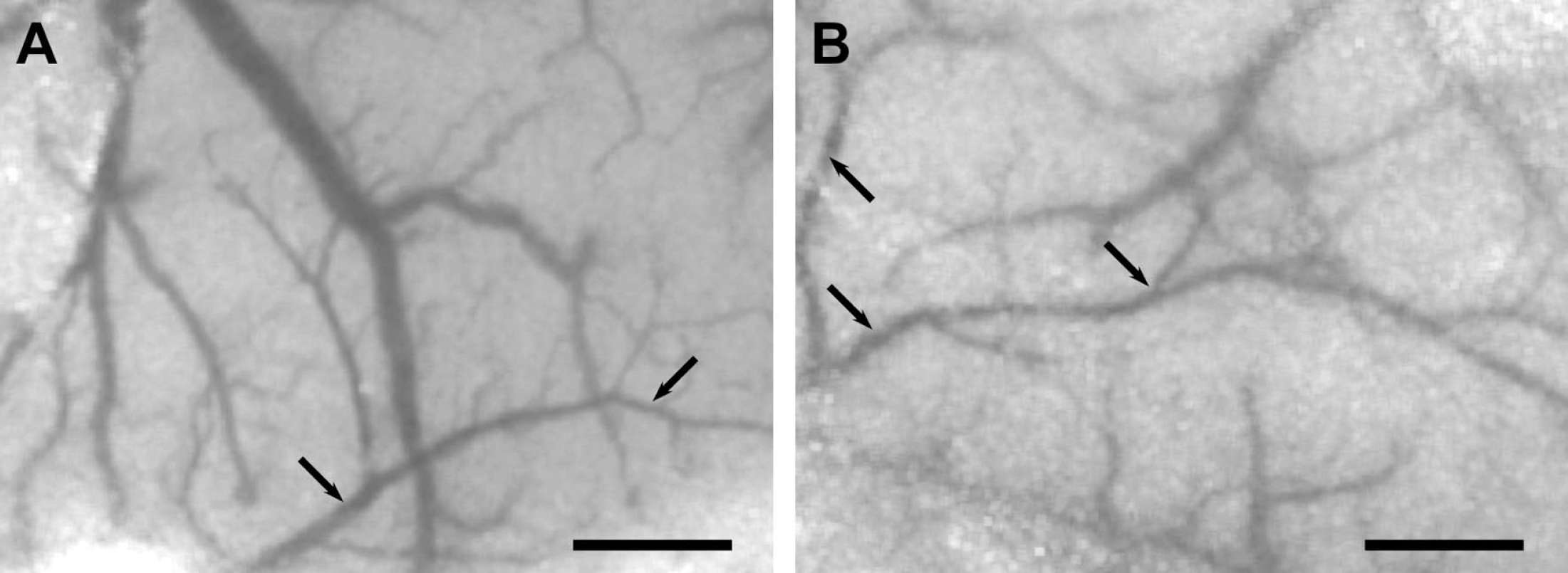
The technique for LSF has been described in detail elsewhere (Dunn et al., 2001). Briefly, a CCD camera (Cohu, San Diego, CA, U.S.A.) was positioned above the head, and a laser diode (780 nm) was used to illuminate the skull surface in a diffuse manner. The penetration depth of the laser is approximately 500 μm from the point laser light hits the tissue. When imaging through intact skull, the laser penetration depth should be calculated from the skull surface. The field of imaging was adjusted to range from 375 × 300 μm to 8 × 6 mm, using a variable magnification objective (×0.75 to ×3, Edmund Industrial Optics, Barrington, NJ, U.S.A.). Raw speckle images obtained in this manner were used to compute speckle contrast (Fig. 1), which is a measure of speckle visibility related to the velocity of the scattering particles. The speckle contrast is defined as the ratio of the standard deviation of pixel intensities to the mean pixel intensity in a small region of the image (Briers and Fercher, 1982). Ten consecutive raw speckle images were acquired at 15 Hz (an image set), processed by computing the speckle contrast using a sliding grid of 7 × 7 pixels, and averaged to improve signal to noise ratio. Speckle contrast images were converted to images of correlation time (τ_c) values, which represent the decay time of the light intensity autocorrelation function. The relationship among speckle contrast, K, and the τ_c is given by

FIG. 1.

Speckle contrast images obtained in mice through either a closed cranial window (A) or intact skull (B). The anatomical detail through the cranial window was better than intact skull; however, arteries (arrows) and veins (arrowheads) were also identified in the intact skull preparation, using anatomical cues and a stereomicroscope. Scale bar = 0.5 mm.

$$K=\frac{{\sigma }_s}{⟨I⟩}={[\frac{{\tau }_c}{2T}\{1-\exp (-2T/{\tau }_c)\}]}^{1/2}$$

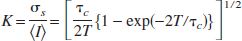
where T is the exposure time of the camera. In theory, the τ_c is inversely and linearly proportional to the mean velocity of the scattering particles (Briers et al., 1999). The precise relationship between τ_c and mean velocity is a complicated function of the light scattering properties of each individual particle and the velocity distribution of the scattering particles (Bonner and Nossal, 1981; Briers et al., 1999), which makes measurement of absolute velocity impractical.

The τ_c values can be used to determine relative changes in CBF velocity. Relative CBF images (percentage of baseline) were calculated by computing the ratio of a baseline image of τ_c values taken before experimental intervention such as hypercapnia or whisker stimulation, with an image at some later time point. At the end of each experiment, mice were sacrificed by exsanguination, and the residual flow value was determined after cardiac arrest and cessation of mechanical ventilation. This value was then taken as the biological zero CBF level, and subtracted from the CBF responses obtained throughout the experiment. In addition to examining relative changes in CBF within one animal, we used the inverse of the computed τ_c values (1/τ_c) as a measure of CBF in arbitrary units, to compare resting CBF between animals.

Thinning of the skull was not performed to avoid irregularities of skull texture or thickness, since these factors can influence the measured relative CBF changes, as well as 1/τ_c. Similarly, drying of the skull during prolonged experiments changed bone translucency and created an uneven texture. Therefore, after reflection of the scalp and periosteum, the skull surface was washed with saline, and then covered with a thin layer of mineral oil to prevent drying. Excess mineral oil was removed to avoid changes in its thickness in time. Mineral oil reduces the effective scattering of the skull and decreases the influence of the skull on the average penetration, by reducing the refractive index variations that lead to scattering. The arteries and veins were identified under stereomicroscopy based on their color and anatomical locations. To determine the changes in CBF, a region of interest (ROI) was placed over different tissue areas. In case of cortical tissue measurements, the ROI (0.1 to 1 mm²) was placed away from cortical vessels. CBF changes in arteries and veins were quantified by placing the ROI over a branch of middle cerebral artery (MCA), or a cortical vein, identified visually from the speckle contrast images. The hypercapnic CBF responses measured by LSF through a cranial window (n = 5) did not significantly differ from those measured through intact skull (data not shown). However, anatomical detail in transcranial speckle contrast images (Fig. 1B) was reduced compared to images obtained through a cranial window (Fig. 1A). Therefore, in transcranial LSF experiments, we routinely measured CBF changes in vessels of at least 25 μm or more in diameter using the x0.75 objective attachment. The size of the ROI was adjusted to be slightly larger than the diameter of the vessel, to integrate changes in vessel caliber. For hypercapnia and autoregulation experiments, three or four separate cortical ROIs were measured and averaged to account for intrinsic variations in CBF response.

Physiologic parameters were within normal limits. Blood pressure at the onset of experiments was comparable under α-chloralose and isoflurane anesthesia (79 ± 3 mm Hg vs. 84 ± 3 mm Hg, respectively, P > 0.1). However, hypercapnia caused a significant reduction in MABP in α-chloralose—anesthetized mice (Table 1), influencing the CBF measurements particularly in the arteries. To account for blood pressure fluctuations during hypercapnia, changes in CBF were converted to changes in cerebrovascular resistance (CVR, % of baseline) according to the following formula: 100(MABP_after/MABP_before)/(CBF_after/CBF_before). By definition CBF_before was taken as 100%.

TABLE 1.

Physiologic parameters before and during hypercapnia

	BP (mm Hg)	pH	pco2 (mm Hg)
Isoflurane
Normocapnia	79 ± 11	7.34 ± 0.04	37 ± 7
Hypercapnia	82 ± 16	7.20 ± 0.03	62 ± 4
α-Chloralose
Normocapnia	70 ± 10*†	7.30 ± 0.12	38 ± 7
Hypercapnia	60 ± 6	7.15 ± 0.09	62 ± 5

*

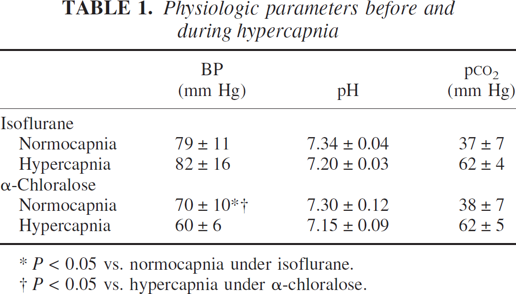
P < 0.05 vs. normocapnia under isoflurane.

†

P < 0.05 vs. hypercapnia under α-chloralose.

Experimental paradigms

Whisker stimulation. Experiments were performed either under isoflurane (n = 8), or α-chloralose (n = 6) anesthesia. Whiskers were trimmed (5 mm) and manually stimulated vertically (i.e., dorsoventral direction) using a cotton tip applicator (4 to 5 Hz, 1 minute), as described previously (Ayata et al., 1996). LSF image sets were averaged for 10 seconds. Whisker stimulation was started after the acquisition of the first image, which was taken as baseline. In this study, we did not attempt to reproduce the precise time course of functional coupling with high temporal resolution, and chose to visualize the acquired images in real-time during whisker stimulation. Hence, there is an apparent delay in the flow increase during whisker stimulation. Two or three ROIs (0.04 to 0.09 mm²) were placed in the whisker barrel field (between 0 to 1 mm posterior, 3.5 to 4.5 mm lateral from bregma), using speckle contrast images to avoid pial vessels. The amplitude of CBF increase was determined by averaging all ROIs. The highest increase in CBF during whisker stimulation was taken as response amplitude, and expressed as percent change from baseline. Whisker stimulation was repeated two or three times in each experiment to determine the maximum response. To better visualize the spatial relationship between the CBF increase during whisker stimulation and the pial vasculature, we used a thresholding paradigm in which 600 speckle images were acquired (10 Hz). Images between 20 and 50 seconds after the onset of whisker stimulation were averaged, and pixels showing more than 10% blood flow increase were superimposed on the speckle contrast image (Fig. 4).

In a separate group of mice (n = 7), we performed simultaneous LDF and LSF measurements. For this purpose, the LDF probe was placed over the whisker barrel cortex, and the laser light from the LDF probe was used to perform LSF. The ROI (100 × 100 μm) for the CBF calculation using LSF was placed at a fixed distance (0.4 mm) from the tip of the LDF probe in a posteromedial direction, to standardize laser intensity from the LDF probe. Consequently, the ROI included both cortical vasculature and capillary bed. At this distance, the ROI remained within the barrel cortex, and the laser light intensity did not saturate the camera.

Hypercapnia.

Hypercapnia was induced by 5% CO₂ inhalation (in 25% O₂, 70% N₂) for 5 minutes under either isoflurane (n = 6) or α-chloralose (n = 6) anesthesia. Arterial blood gas samples were obtained just before the onset and then at the termination of hypercapnia. The hypercapnic end-tidal CO₂ was usually between 7% and 8%, corresponding to an arterial pco₂ of 55 to 65 mm Hg. LSF images were obtained every 30 seconds, for a total of 20 images. The first two images were taken as baseline flow, and the highest increase during hypercapnia was taken as the response amplitude in each animal. Hypercapnia was repeated twice during each experiment to determine the average maximum response. CO₂ reactivity index was calculated by dividing the maximum increase in CBF (%) to the increase in arterial pco₂ (mm Hg) during hypercapnia.

Autoregulation.

Experiments were performed either under isoflurane (n = 6) or α-chloralose (n = 6) anesthesia. The upper limit of autoregulation was determined by intraperitoneal injection of phenylephrine at doses of 5 to 50 μg to stepwise elevate the MABP by approximately 10 mm Hg at a time, up to 150 mm Hg; increasing the MABP above this level frequently resulted in pulmonary edema and altered acid-base status, and was therefore not attempted. LSF images were obtained 2 to 4 minutes after a stable MABP level was achieved. CBF at a MABP of 80 mm Hg was taken as 100%, and subsequent changes were expressed relative to this value. The lower limit of autoregulation was determined by withdrawing blood from the arterial line to lower the mean arterial pressure by 10-mm Hg steps, allowing 3 to 5 minutes between the blood draws for stabilization. The upper and lower limits of autoregulation were determined by comparing CBF at each MABP level to baseline (i.e., CBF at 80 mm Hg), using one-way analysis of variance. The upper limit of autoregulation was taken as the MABP above which CBF was statistically significantly increased compared with CBF at a MABP of 80 mm Hg. Similarly, the lower limit of autoregulation was taken as the MABP below which CBF was statistically significantly decreased compared to CBF at a MABP of 80 mm Hg.

Resting CBF measurement using the [14C]iodoamphetamine technique

In these series of experiments, apoE-knockout mice (15 ± 3 weeks old, n = 4, and 60 ± 23 weeks old, n = 3) were used in addition to C57BL/6J (21 ± 10 weeks old, n = 4). In preliminary experiments, we observed that apoE-knockout mice had lower resting CBF values compared with wild-type mice (unpublished data); therefore, we aimed to determine how well LSF and [¹⁴C]iodoamphetamine techniques correlated under these conditions. For this, we first performed LSF and calculated the 1/τ_c, and then determined absolute resting CBF in the same animal using [¹⁴C]iodoamphetamine technique under α-chloralose anesthesia (Betz and Iannotti, 1983; Van Uitert and Levy, 1978), with minor modifications (Fujii et al., 1997; Yamada et al., 2000). The left femoral artery and jugular vein were cannulated. After determining MABP and blood gases, arterial blood was withdrawn continuously from the femoral artery at a rate of 0.3 mL/min. Then, 1 μCi of N-isopropyl-[methyl-1,3-¹⁴C]-p-iodoamphetamine in 0.1 mL saline was bolus injected into the external jugular vein over 10 seconds. Twenty seconds after injection, the animal was decapitated and the blood withdrawal terminated simultaneously. The brain was removed quickly, frozen in isopentane on dry ice, and the cortex was dissected. After adding Scintigest and incubating (50°C for 6 hours), scintillation fluid and H₂O₂ were added. Twelve hours after shaking, radioactivity in brain and blood were measured by liquid scintillation spectrometry. CBF was calculated according to previously described methods (Betz and Iannotti, 1983; Van Uitert and Levy, 1978).

Focal cerebral ischemia

Focal cerebral ischemia was induced by distal MCA occlusion. After general surgical preparation, mice were placed in a stereotaxic frame, and skull surface was prepared for LSF as described earlier. The temporalis muscle was separated from the temporal bone and removed. A burr hole (2 mm diameter) was drilled under saline cooling in the temporal bone overlying the MCA just above the zygomatic arch. The dura was kept intact and a 10–0 nylon suture was passed through the cortex behind the MCA just proximal to its bifurcation. The suture was then loosely tied and brain surface was covered with saline. In preliminary experiments we determined that passage of the suture behind the MCA uniformly induced one cortical spreading depression; therefore, after the placement of the suture we waited for 1 hour before ligating the MCA to allow the CBF changes induced by spreading depression to resolve. LSF imaging was started 1 minute before MCA ligation and continued throughout the experiment. A thresholding paradigm similar to that used for the spatial analysis of whisker response was applied by setting the threshold at 50% or less residual CBF compared to preischemic baseline. In addition, CBF profiles were generated along the mediolateral axis to determine the ischemic CBF gradient in the cortex.

Data acquisition and analysis. Blood pressure and end-tidal CO₂ were continuously recorded and analyzed using PowerLab (ADInstruments). Paired or unpaired Student's t-test was used to compare cortical capillary and arterial flow, and the effects of different anesthetics, respectively. Two-way repeated measures analysis of variance followed by Tukey multiple comparison test were used to determine the upper and lower limits of autoregulation and the effect of anesthetics. Results were expressed as percent change from baseline (± standard deviation). Regression analysis was used to test the correlation between 1/τ_c values and absolute CBF.

RESULTS

Whisker stimulation

Whisker stimulation increased CBF in the barrel cortex with an amplitude similar to previous observations using LDF (Fig. 2, Table 2) (Ma et al., 1996a; Wolf et al., 1997). The hyperemic response did not differ between animals anesthetized with α-chloralose (n = 6) or isoflurane (n = 8). The maximum response was usually reached within 20 seconds after the onset of whisker stimulation (Fig. 3). The maximum increase in CBF was similar when LDF and LSF measurements were obtained simultaneously within the same barrel field during whisker stimulation (21% ± 10% vs. 17% ± 5% for LDF and LSF, respectively; n = 7, P > 0.1). The peak CBF increases were recorded 0.5 to 1 mm posterior, and 3 to 4 mm lateral to bregma, corresponding to barrel fields as previously described (Woolsey and Van der Loos 1970). Furthermore, the blood flow changes were significantly higher within the MCA branches supplying the barrel cortex than within the barrel cortex capillary bed (27% ± 11% vs. 19% ± 8%, respectively, n = 14, isoflurane and α-chloralose groups combined, P < 0.05; Fig. 3, Table 2). As shown in Fig. 3, CBF often increased in regions adjacent to the barrel cortex, albeit to a lesser extent, and this variability seemed unrelated to differences in level of anesthesia, or arousal.

FIG. 2.

Whisker stimulation-induced hyperemia in barrel cortex. Entire whisker pad was manually stimulated for 1 minute at a frequency of 4 to 5 Hz. (A) Imaging field with respect to mouse skull, showing the approximate location of whisker barrel field (dashed lines). Scale bar = 1 mm. (B) Pseudocolor images of regional CBF elevations corresponding to whisker barrel fields, shown in panel A. A smaller increase was present in adjacent cortical fields, but not detected farther away (not shown). Color bar represents CBF as percent of baseline.

FIG. 3.

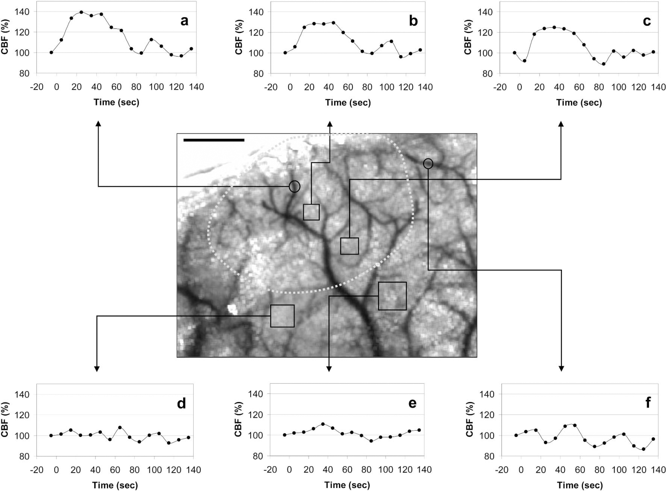
The time course of whisker stimulation-induced increase in CBF measured at six different ROIs using LSF. Whisker stimulation started between 0 and 10 seconds, and ended at 60 seconds. The LSF tracings are the average of two whisker stimulation trials in one mouse. Differential measurements were obtained from middle cerebral artery branches (circular ROIs) supplying either the barrel cortex (a) or outside (f), and from cortical capillary bed (square ROIs), either within the barrel cortex (b, c), or outside (d, e). Area marked by the dashed line indicates the approximate location of whisker barrel cortex (Woolsey and Van Der Loos, 1970). The amplitudes of measured CBF increases were typically smaller than the individual peaks identified in the two-dimensional flow map because of averaging within the ROI. Scale bar = 1 mm.

FIG. 4.

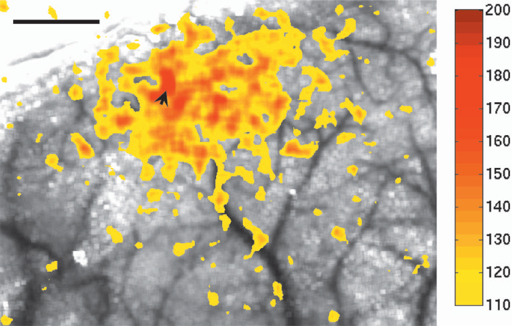
Whisker stimulation-induced relative increase in CBF (thresholded at 10% CBF increase) superimposed on the speckle contrast image of cortex and pial vasculature transcranially, to show the spatial relationship of flow increase and cortical surface structures. The earliest and highest increase was within an MCA branch (arrowhead). This type of thresholding allows detailed spatial analysis of functionally activated cortical fields. Color bar shows CBF as percent of baseline. Scale bar = 1 mm.

TABLE 2.

Cerebral blood flow response to whisker stimulation

	Cortex	Artery
Isoflurane	19% ± 6%	26% ± 9%*
α-Chloralose	19% ± 10%	28% ± 13%*

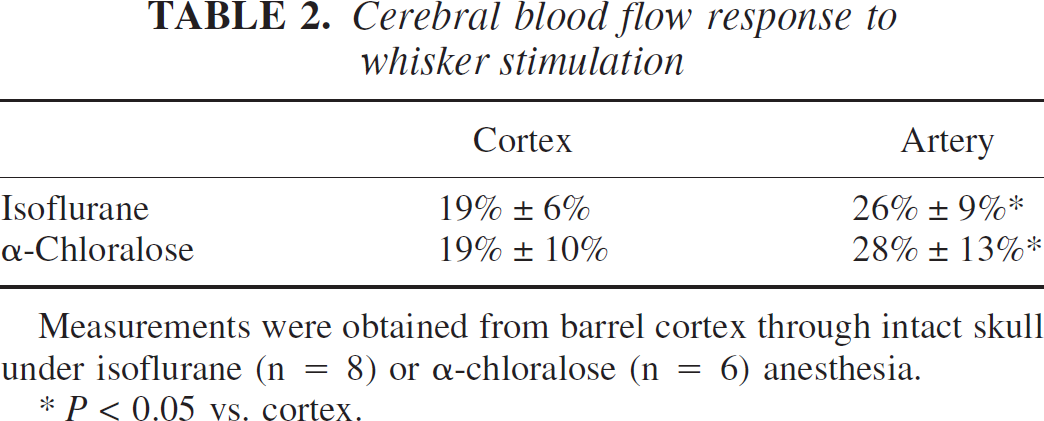
Measurements were obtained from barrel cortex through intact skull under isoflurane (n = 8) or α-chloralose (n = 6) anesthesia.

*

P < 0.05 vs. cortex.

Hypercapnia

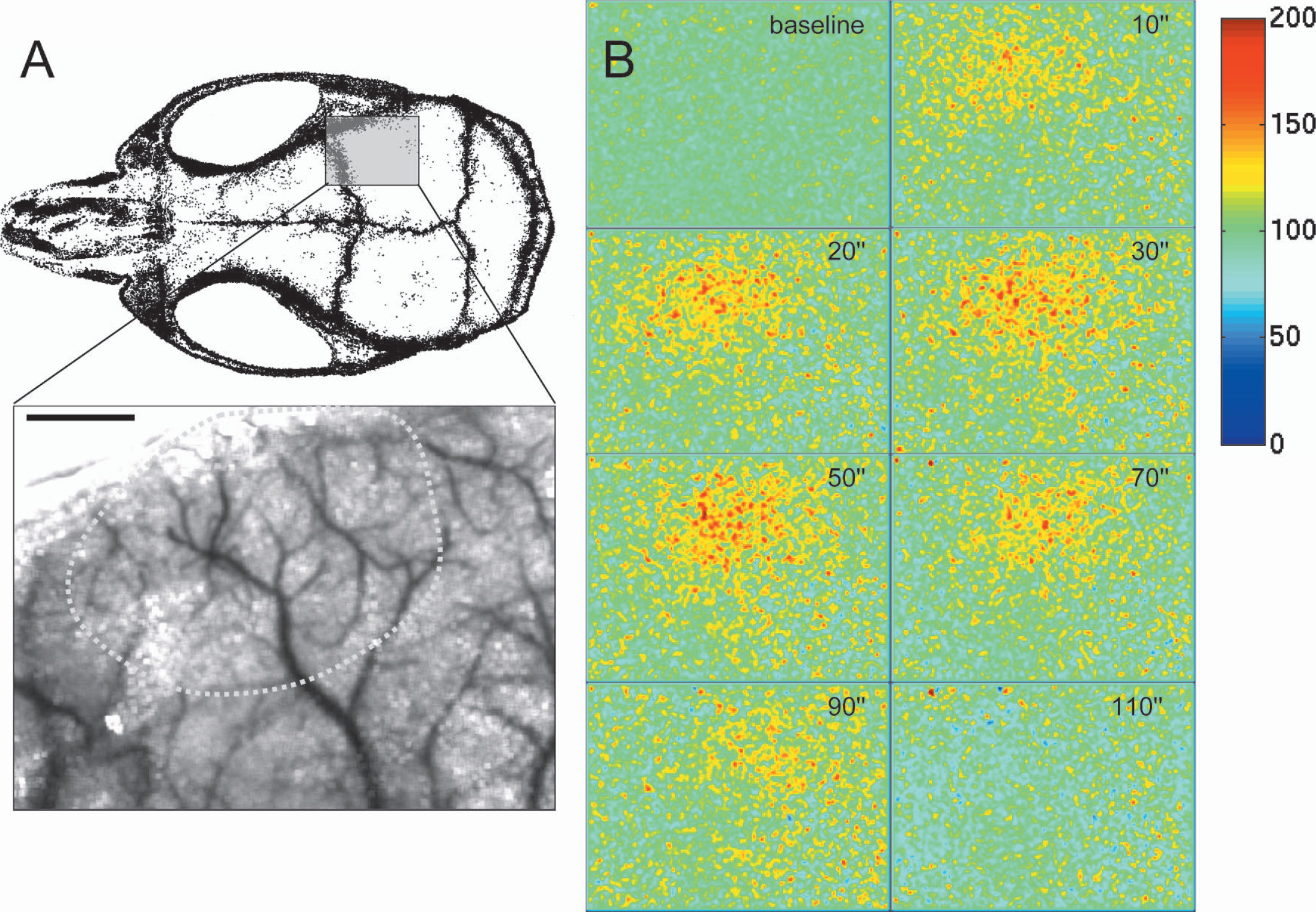
Breathing 5% CO₂ (pco₂ approximately 60 mm Hg, Table 1) in α-chloralose—anesthetized mice caused a global increase in CBF and decrease in CVR (Fig. 5, Table 3), similar in amplitude to our previous observations using LDF (Dalkara et al., 1995; Ma et al., 1996b). The CO₂ reactivity index was 1.4 ± 0.3, compared to a previously published value of 1.8 (Dalkara et al., 1995). CBF increase was slightly larger in pial arteries and veins, although this difference did not reach statistical significance (P > 0.05, n = 6, Table 3). Hypercapnic hyperemia was attenuated by 63% in animals anesthetized with isoflurane (n = 6) compared with α-chloralose (n = 6, P < 0.05) (Table 3).

FIG. 5.

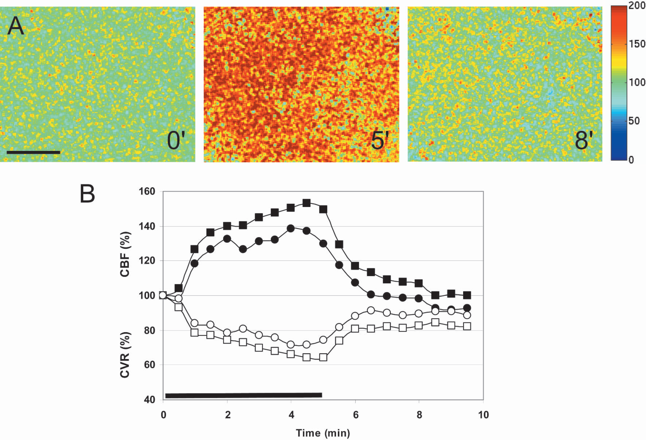
Hypercapnic hyperemia in mouse parietal cortex. (A) Pseudocolor images showing a relatively homogeneous increase in CBF throughout the cortex, taken at baseline, 5 and 8 minutes after the onset of hypercapnia (5% for 5 minutes). The flow increase in arteries was not significantly different than the cortex (scale bar = 0.5 mm). Color bar shows CBF as percent of baseline. (B) The time course of hypercapnic hyperemia in a representative experiment. Measurements were obtained every 30 seconds. Circle, artery; square, cortex; filled symbols, CBF; clear symbols, CVR. Horizontal bar represents hypercapnia.

Autoregulation

The upper and lower MABP limits for CBF autoregulation were 110 and 40 mm Hg, respectively, when measured by LSF in α-chloralose—anesthetized mice (n = 6, Fig. 6). Isoflurane anesthesia completely abolished the ability to maintain constant CBF with changes in MABP (n = 6).

FIG. 6.

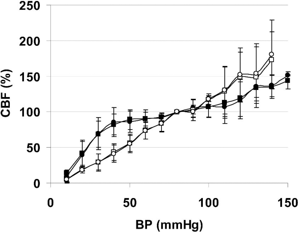
Autoregulation of CBF in mouse cortex. Phenylephrine (intraperitoneal), and controlled bleeding were used to elevate or lower the blood pressure by approximately 10 mm Hg at a time. Statistically significant differences from the baseline CBF readings were observed at 120 and 40 mm Hg under α-chloralose anesthesia. Isoflurane abolished autoregulation. Circle, artery; square, cortex; filled symbols, α-chloralose anesthesia; clear symbols, isoflurane anesthesia.

TABLE 3.

Hypercapnic hyperemia under isoflurane or α-chloralose anesthesia

	ΔCBF (%)			ΔCVR (%)Cortex
	Cortex	Artery	Vein	Cortex	Artery	Vein
α-chloralose	38 ± 25*	43 ± 31*	44 ± 34*	–37 ± 9†	–38 ± 13†	–40 ± 9†
Isoflurane	14 ± 7	17 ± 9	14 ± 9	–6 ± 7	–9 ± 6	–6 ± 6

*

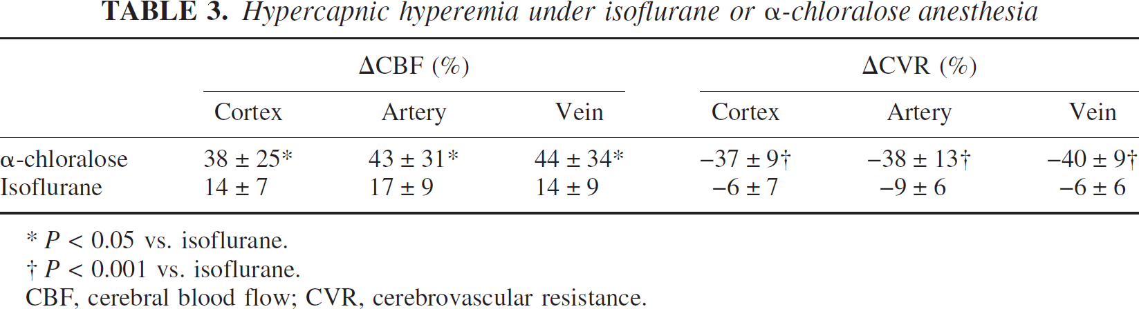
P < 0.05 vs. isoflurane.

†

P < 0.001 vs. isoflurane.

CBF, cerebral blood flow; CVR, cerebrovascular resistance.

Correlation time values and resting CBF

Because the contact properties between the LDF probe and tissue are highly variable, LDF does not measure resting CBF reliably and therefore cannot be used to compare baseline data between animals. Once the LDF probe is moved, the baseline is no longer reliable. The correlation time (τ_c) values represent the decay time of the light intensity autocorrelation function obtained from speckle contrast images. To validate the inverse correlation time (1/τ_c) as a measure to compare resting CBF between different animals, we first determined the 1/τ_c values from the entire dorsal cortical surface, and then performed absolute CBF measurements using the [¹⁴C]iodoamphetamine technique in the same animal. There was a linear relationship between the absolute CBF (range studied 75 to 130 mL · 100 g⁻¹ · min⁻¹) and 1/τ_c values obtained from the same hemisphere (R² = 0.77, P < 0.001, Fig. 7). Furthermore, repeated measurements of 1/τ_c values from individual brain regions within a single animal were highly reproducible under stable physiologic conditions (standard deviation ≤ 10% of mean). In a separate group of mice, we showed that resting 1/τ_c in mice anesthetized with α-chloralose was approximately half of resting 1/τ_c in mice anesthetized with isoflurane (5,186 ± 2,514 s⁻¹ [n = 6] vs. 9,600 ± 2,936 s⁻¹ [n = 10], respectively; P < 0.01). This finding was consistent with the previously published effects of isoflurane to increase resting CBF by about 30%, and α-chloralose to reduce it by 30%, at the doses used in this study (Kehl et al., 2002; Lenz et al., 1998; Okamoto et al., 1997; Szabo et al., 1983).

FIG. 7.

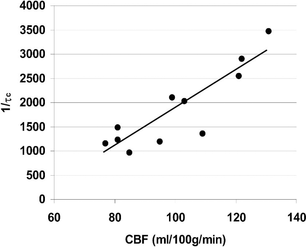
Relationship between inverse correlation time values (1/τ_c) obtained from LSF, and absolute cortical blood flow determined using [¹⁴C]iodoamphetamine technique under resting state (regression analysis, P < 0.001). To calculate the τ_c values, five LSF image stacks were obtained every 30 seconds and averaged, approximately 5 minutes before decapitation, for absolute resting CBF measurements using the [¹⁴C]iodoamphetamine technique. Each data point represents one animal.

Focal cerebral ischemia

Distal MCA ligation caused an abrupt CBF decrease within the MCA territory (Fig. 8, n = 5). To determine the cortical regions with moderate to severe ischemia, we applied a thresholding paradigm such that regions of cortex with 50% or less residual CBF (compared with preischemic baseline) were highlighted and superimposed on the speckle contrast image (Fig. 9A). At 1 minute after MCA ligation, ischemic cortex with 50% or less residual CBF extended from 2.5 mm anterior to bregma to 2.5 mm posterior, in anteroposterior axis, and from 2 mm lateral from midline to the hemispheric edge, in mediolateral axis (Fig. 9A). To determine the gradient of CBF reduction after distal MCA ligation, we quantified the percent reduction in CBF along the mediolateral axis at the level 0.6 mm posterior to bregma, and averaged the CBF profiles (Fig. 9B). By doing this we found that, flow within anterior cerebral artery territory (i.e. medial 1 mm of cortex) consistently showed a 10 to 20% reduction in CBF immediately after distal MCA occlusion. More laterally, residual CBF within the MCA territory declined from 80% to 30% of preischemic baseline between 1.2 and 2.2 mm lateral from midline (at the level of 0.6 mm posterior to bregma; Fig. 9B, vertical lines). The residual blood flow in the ischemic core was probably due to collateral blood supply from branches of MCA proximal to the occlusion site as well as from anterior cerebral artery; however, a contribution from the blood flow within the dura and skull cannot be excluded.

FIG. 8.

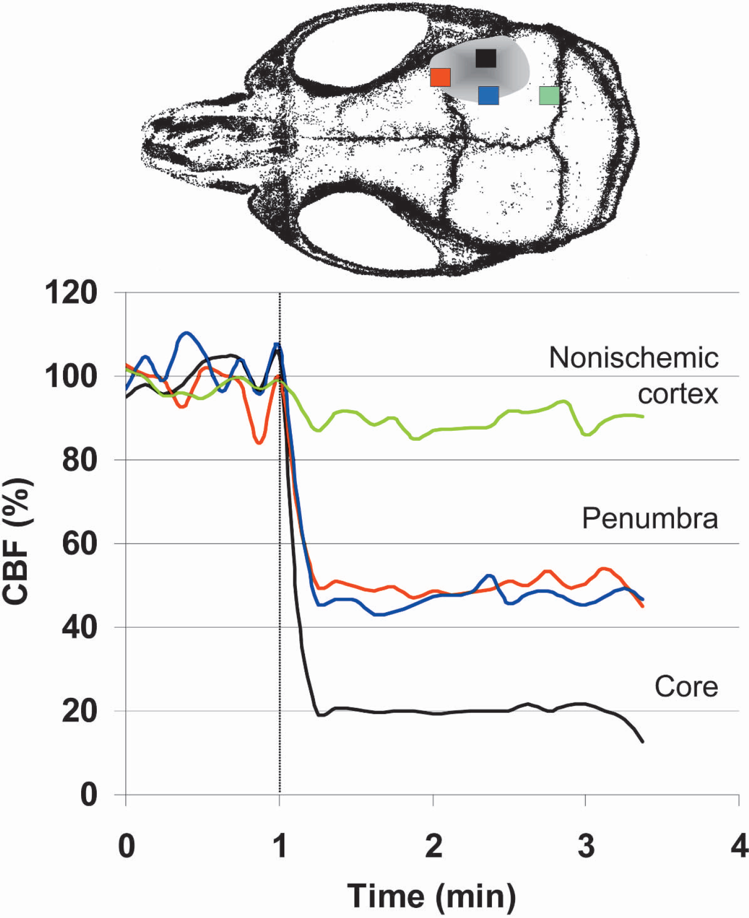
Time course of CBF changes during the first 2 minutes of distal MCA occlusion (dashed line). Shaded area indicates the approximate location of the ischemic cortex. Four regions of interest were placed in the core (black), penumbra (red and blue), and nonischemic cortex (green) to quantify the CBF changes. CBF in the ischemic core abruptly dropped to 20% of baseline immediately after MCA occlusion. Penumbral CBF reduction was milder at approximately 50% of baseline, whereas nonischemic cortex had normal CBF.

FIG. 9.

(A) Two-dimensional map of CBF changes 1 minute after distal MCA occlusion through a temporal craniotomy (arrow) from a representative experiment. The imaging field was located on the right hemisphere (A, anterior; P, posterior; L, lateral; S, sagittal suture). The axis labels indicate distance from midline (vertical axis), or from bregma (horizontal axis), in millimeters. The blue highlight indicates the spatial distribution of ischemic cortex with ≤50% residual CBF compared with preischemic baseline. Thresholded relative CBF image was superimposed on the speckle contrast image. Color bar shows CBF as percent of baseline (B) The relative CBF profile 1 minute after distal MCA occlusion plotted along the mediolateral axis at 0.6 mm posterior to bregma (n = 3). Three zones are identified based on the CBF gradient: a) the medial cortex with normal CBF (80 to 100% of baseline CBF); b) the steep portion of the ischemic CBF drop from 80% to 30% of baseline CBF (i.e., “hemodynamic penumbra”); and c) a uniform and severe reduction in CBF at the center of ischemic cortex (20 to 30% of baseline CBF; i.e., “hemodynamic core”).

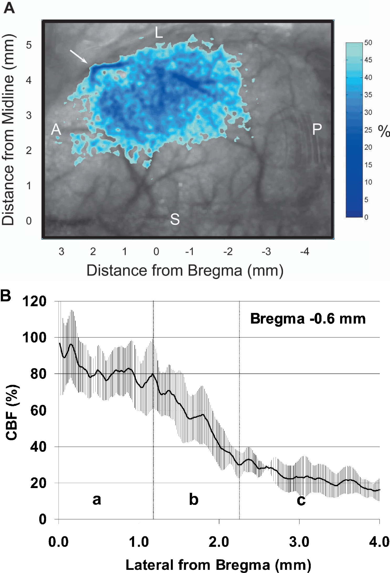
DISCUSSION

We showed that LSF reproduces the magnitude of well-known cerebrovascular responses to metabolic activation, hypercapnia, and changes in blood pressure (i.e., autoregulation), previously studied using LDF. In addition, we showed in real-time the two-dimensional regional CBF increase in barrel cortex in response to stimulation of all whiskers, and illustrated the flow changes through an intact mouse skull. Furthermore, by achieving a high spatial resolution, we could differentially study the degree of CBF changes within the cortical capillary bed or pial vasculature. Finally, we mapped the early ischemic CBF changes in a distal MCA occlusion model with high spatial resolution.

The laser speckle technique is primarily a measure of the velocity of scattering particles (i.e., red blood cells); however, in practice, we consistently observed a close agreement in the amplitude of CBF changes between laser speckle and LDF in a variety of paradigms including functional activation and hypercapnia. Therefore, our study suggests that LSF is comparable to LDF for the study of physiologic changes in CBF.

Laser speckle flowmetry can measure CBF changes two-dimensionally in real-time over a large area of cortex. Its spatial resolution is determined by the laser wavelength, the quality of the optics, the optical properties of the tissue, and the amount of pixel averaging to estimate the speckle contrast. For our experimental conditions, the pixel size is 4 to 13 μm, depending on the level of optical magnification (x3 to x0.75), which is better than most currently available laser-Doppler scanners. The field of view can be adjusted from less than 1 mm to several centimeters. While the theoretical temporal resolution of LSF is currently limited by the frame rate of the camera, in practice the signal-to-noise ratio requires averaging sequential camera frames, thus reducing temporal resolution, and/or averaging separate experimental trials. If online visualization of the acquired images is desired, imaging speed is limited by the computer processing speed. The need for averaging arises because of the relatively high noise level in LSF, due to physiologic variations such as heartbeat and respiration. Since the speckle pattern is highly motion sensitive, any motion artifact alters the speckle contrast. This constitutes one of the advantages of imaging through an intact skull, where brain pulsations reflecting arterial or intrathoracic pressure fluctuations are minimized; for this reason, a closed cranial window is preferred over an open one, when a higher resolution is needed. Recording in an intact skull preparation also avoids surgical trauma and brain temperature fluctuations, and prevents cortical swelling and herniation during hyperemic responses. However, spatial resolution is reduced when imaging through an intact skull, and only those vessels larger than 25 μm in diameter can be reliably measured using the described setup.

Although LSF is conceptually simple, and easy to implement, several issues deserve comment. To ensure proper sampling of the speckle pattern, the aperture of the imaging lens must be set correctly, which determines the speckle size at the camera plane (Briers, 2001). For example, if the aperture is too wide, multiple speckles will be imaged onto a single pixel resulting in artificially low speckle contrast values. The optimal aperture setting, defined in terms of the numerical aperture (NA) of the imaging system is given by NA = 1.22ΛM/d_p, where d_p is the size of a pixel, Λ is the wavelength of light, and M is the magnification. When the aperture is set at its optimal value, the size of the speckles matches the size of the pixels so that each pixel samples only one speckle. Therefore, when the magnification is changed, the aperture setting must also be changed. One consequence is that the light level at the camera cannot be adjusted by changing the aperture since the aperture is set by the above equation. Instead, light level at the camera can be adjusted by changing the output power of the laser source.

Laser-Doppler flowmetry and related techniques provide relative measurements of temporal variations in CBF, and therefore cannot be used to compare resting CBF between individual or groups of animals. This limitation is mainly due to variations in the surface properties between the LDF probe and the tissue studied, as well as variations in the complex microvascular structures sampled by LDF, and can only be overcome by averaging a large number of measurements (Soehle et al., 2001). In this study we showed that the correlation time (τ_c) values for speckle fluctuations are highly reproducible, and can be used to compare resting CBF between animal groups. To validate the use of τ_c values, we compared CBF obtained by the quantitative [¹⁴C]iodoamphetamine technique to CBF as estimated by 1/τ_c. The correlation was highly significant within the range of CBF values studied (75 to 130 mL · 100 g⁻¹ · min⁻¹; P < 0.001, Fig. 7). However, we cannot rule out the possibility of deviation from linearity at extremely high or low CBF levels. Therefore, the relationship shown in Fig. 7 is not intended to be complete over ranges of CBF outside 75 to 130 mL · 100 g⁻¹ · min⁻¹, but shows the feasibility of using 1/τ_c values as a screening tool to estimate the differences in resting CBF between groups of animals. This was exemplified by comparing the resting 1/τ_c values in α-chloralose– or isoflurane-anesthetized mice. More experiments are required to determine the exact relationship between 1/τ_c and absolute CBF over a wider range of CBF values. We noted that several factors influenced the 1/τ_c values: the optical magnification level, the laser light intensity, and variations in the refractive properties of intact skull. Therefore, if one desires to use correlation time values to compare resting CBF between animals, the optical magnification, the intensity of surface illumination, and the skull thickness must be identical between groups. Furthermore, surface illumination should be even throughout, and measurements must be obtained from areas with uniform translucency.

Whisker stimulation-induced blood flow increase within arteries supplying the barrel cortex was larger (28%) compared with the increase in capillaries (19%). One explanation for this finding is that a few arteriolar branches provide the increased flow to entire barrel cortex, and therefore the flow increase is concentrated, yielding a larger change. Our data showed a similar trend for larger arterial blood flow increases in hypercapnia, where blood flow increase is global, but the difference between the two did not reach statistical significance (Table 3). We used a ROI slightly larger than the arteriolar diameter to detect vasodilation in addition to increased blood flow velocity (Cox et al., 1993). We also used a CBF thresholding paradigm to perform a spatial analysis of the whisker response (Fig. 4) to determine the recruitability of cortex during sensory stimulation. Previous studies of functional activation have focused on CBV changes using intrinsic optical signals, as well as reflectance spectroscopy to determine hemoglobin oxygenation (Jones et al., 2001, 2002; Lindauer et al., 2001).

Interestingly, the whisker responses we measured over the capillary bed in barrel cortex were somewhat smaller, whereas arterial blood flow increases were larger, compared with our previous data using LDF in mice (24%) (Ayata et al., 1996). One potential explanation for this discrepancy is volume averaging by LDF. The LDF probe measures flow in pial arterioles as well as cortical tissue, even if the probe is deliberately placed away from major vessels. Therefore, LDF measures an integrated response within the capillary bed and pial arterioles during hyperemia. Our data suggest that LDF detects a greater arteriolar contribution than LSF. The choice and depth of anesthesia, and the penetration depth of laser light, may also have contributed to differences from prior studies in mice (Gotoh et al., 2001; Lindauer et al., 1993, 1999; Ma et al., 1996a).

The penetration depth of the detected light is a complicated function of the tissue optical properties (scattering coefficient, scattering anisotropy, and absorption coefficient). Using Monte Carlo simulations, we estimated that the penetration depth of the detected photons can be up to 1 to 2 mm, which is consistent with other analyses of the same imaging geometry (Kohl et al., 2000). However, although a portion of the detected light does penetrate to these depths, the penetration depth at any pixel contains a wide distribution. This distribution is weighted towards the surface, and therefore, the average penetration depth is 0.5 to 0.75 mm for the assumed optical properties (scattering coefficient μ_s = 100 cm⁻¹, scattering anisotropy g = 0.9, absorption coefficient μ_a = 0.01 cm⁻¹), from the point laser light first hits the tissue.

Finally, using the excellent spatial and temporal resolution provided by LSF, we developed a distal MCA occlusion model where CBF changes can be mapped through the intact skull before, during, and after occlusion in mice. By using this approach, we found that there is a segment of cortical tissue at the margins of a focal ischemic lesion wherein the CBF decreases steeply from 80% to 30% (Fig 9B, “b”). We believe this region represents the border zone between anterior and MCA, and reflects the underperfused tissue at risk. The term “hemodynamic penumbra” aptly describes this zone. According to this scheme, hemodynamic penumbra represents brain tissue that lies between the border of tissue originally supplied by the occluded artery, and the farthest point where blood flow from collateral arteries can reach. By studying the hemodynamic penumbra with high temporal and spatial resolution, LSF provides an opportunity to examine the natural evolution of ischemic injury and the utility of potential treatments.

In summary, we showed that LSF is highly suitable to study cerebrovascular physiology in mice. It provides excellent spatial resolution, even through intact skull, allowing identification and measurement of blood flow changes within pial vasculature, separate from the cortical capillary bed. The size of imaging field is adjustable, making it possible to study CBF within a single cortical whisker barrel (Dunn et al., 2003) or in the entire brain, including all vascular territories bilaterally and simultaneously, without sacrificing spatial resolution. LSF has a temporal resolution approaching real-time, allowing monitoring of rapid changes in blood flow, such as arterial occlusion, and metabolic coupling upon functional cortical activation. When applied to a distal MCA occlusion model, LSF can quantify the ischemic burden and its time course. In addition, LSF can be used to make comparisons of resting CBF between animal groups, an advantage over LDF. Among potential applications of LSF, those models with significant spatial heterogeneity in CBF changes (e.g., focal cerebral ischemic penumbra, functional activation), or those with intrinsic arterial pathology (e.g., cerebral amyloid angiopathy, CADASIL, atherosclerosis), are the conditions where LSF may be most beneficial.