
Abstract
The graphical analysis method, which transforms multiple time measurements of plasma and tissue uptake data into a linear plot, is a useful tool for rapidly obtaining information about the binding of radioligands used in PET studies. The strength of the method is that it does not require a particular model structure. However, a bias is introduced in the case of noisy data resulting in the underestimation of the distribution volume (DV), the slope obtained from the graphical method. To remove the bias, a modification of the method developed by Feng et al. (1993), the generalized linear least squares (GLLS) method, which provides unbiased estimates for compartment models was used. The one compartment GLLS method has a relatively simple form, which was used to estimate the DV directly and as a smoothing technique for more general classes of model structures. In the latter case, the GLLS method was applied to the data in two parts, that is, one set of parameters was determined for times 0 to T1 and a second set from T1 to the end time. The curve generated from these two sets of parameters then was used as input to the graphical method. This has been tested using simulations of data similar to that of the PET ligand [11C]-d-threo-methylphenidate (MP, DV = 35 mL/mL) and 11C raclopride (RAC, DV = 1.92 mL/mL) and compared with two examples from image data with the same tracers. The noise model was based on counting statistics through the half-life of the isotope and the scanning time. Five hundred data sets at each noise level were analyzed. Results (DV) for the graphical analysis (DV
The interpretation of positron emission tomography (PET) data in physiologic terms is dependent upon the estimation of model parameters. These model parameters which incorporate the effects of both the tissue uptake and the plasma delivery of the tracer are used to quantify PET data and thus allow intersubject comparisons. The nonlinear least squares (NLS) methods can provide statistically accurate estimates of model parameters. These methods, which are based on a particular model structure, generally require considerable computation time. The linearized version of the standard compartment models (Blomqvist, 1984; Evans, 1987) provide a more efficient method of parameter estimation. Graphical analysis represents a further simplification in which the set of linear equations is transformed into a linear plot (Logan et al., 1990). Although this is applicable to a multicompartment system, only two parameters are determined, the slope and the intercept, which are combinations of the model parameters. In the case of reversibly binding ligands, the slope is the distribution volume (DV). The strength of the graphical analysis is that it does not require a particular model structure since in many cases one model may not equally fit all data sets from the same structure and region of interest. When the model structure does not quite fit the data, a bias can be introduced into the model parameter of comparison, generally the distribution volume (DV). In the case of noisy data, the linearized equations can also introduce a bias, because the error term at any given time point also contains the error terms at the earlier time points (Feng et al., 1993, 1996). As a result, the graphical method on average will underestimate the DV and this underestimate is greater with larger DVs (Hsu et al., 1997; Slifstein and Laruelle, 1999; Abi-Dargham et al., 2000). However, the effect on any given data set depends upon the nature of the noise; for example, when one particular data set deviates in a seemingly nonrandom way from the “true” data (Figs. 2A and 3A), all analysis methods will exhibit an apparent bias. This can only be addressed by reducing the noise source in the data or averaging over data sets, etc.
Feng et al. (1996) have developed a solution to the bias problem in the case of specific compartmental models called the generalized linear least squares (GLLS) method. In the case of the one-tissue compartment model, there are two parameters to be estimated and the GLLS equations for parameter estimation take on a relatively simple form involving the inversion of a 2 × 2 matrix. This one-compartment GLLS method was adapted to use as a smoothing technique for more general classes of model structures. This is accomplished by applying the GLLS method to the data in two parts, that is, to determine one set of parameters for times 0 to T1 and a second set from T1 to the end time. The curve generated from these two sets of parameters can then be used as input to the graphical method to generate an unbiased estimate of the DV. This has been tested using simulations of data similar to that of the PET ligands [11C]raclopride which binds to the D2 receptor (Volkow et al., 1993) and [11C]-d-threo-methylphenidate which binds to the dopamine transporter (Volkow et al., 1995). This combination of the GLLS method and the graphical method provides the possibility of retaining the model independent type of analysis without the bias inherent in the linear methods while still maintaining a fairly simple method of analysis. Results from this method are compared with the DV calculated directly from the solution to the one-compartment GLLS method and to the NLS method as well as to graphical analysis without smoothing.
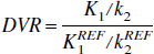
This method was also applied to the simplified reference tissue model of Lammertsma and Hume (1996) and Gunn et al. (1997). The equation was modified to allow a linear solution for k2 as in Feng's method. Estimates of three parameters were generated in this case as opposed to two when the input function is measured. The same two part procedure was used to smooth the data as was done with the DV and the graphical method was applied to the smoothed data using the reference region and an average efflux constant (Logan et al., 1996). This was compared to the graphical method without smoothing and to the distribution volume ratio (DVR) determined directly from the linear solution of the simplified reference tissue model (Lammertsma and Hume, 1996).
The input function and reference tissue techniques were also applied to human PET data from a 11C raclopride (RAC) and [11C]-d-threo-methylphenidate (MP) study using regions from the basal ganglia where both tracers concentrate.
Theory
The one-tissue compartment model is described by
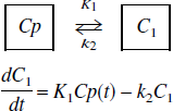
where Cp(t) is the plasma tracer concentration at time, t; C1 is the tissue tracer concentration; K1 and k2 are the transport constants, plasma to tissue and tissue to plasma, respectively. The linear form of this model is the set of equations (for scan times t1)
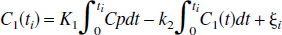
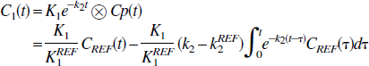
where the equation errors, ζ i , are not statistically independent because each succeeding one depends upon the previous ones. This can result in biased parameter estimates (Feng et al., 1996). To overcome the bias problem in the solution of the one-compartment model, Feng et al. (1993) introduced the GLLS method that removes the bias. The GLLS form of Eq. 1b is
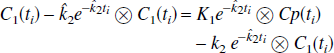
where ⊗ denotes convolution and C1 (t) is the measured tissue tracer concentration. This can be written in matrix form as

where
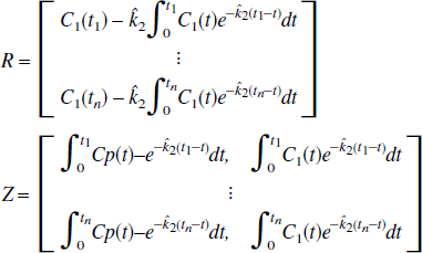
The solution is
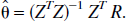
The parameter
Because the one-compartment model is somewhat restrictive, the above procedure was adapted to be applicable to a general PET data set and does not require a particular model structure. This is to be accomplished by applying the GLLS method for one-compartment to the data in two parts-that is, determine one set of parameters for times 0 to T1 and a second set of parameters for T1 to the end. The equation analogous to Eq. 2a for times ti > T1 is
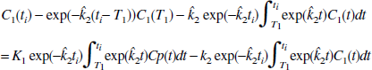
Using the two sets of ĥ to generate a “smoothed” time-activity data set, the simple GLLS model of Eq. 2 will be tested to see if it can approximate data from more complex models. Applying the graphical method for reversible tracers to the smoothed data set should generate an unbiased estimate of the distribution volume (DV), if this smoothing technique is valid.
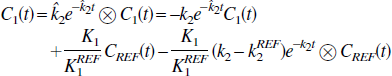
This procedure can be extended to the graphical analysis with a reference region. Using for the reference region
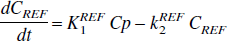
and substituting for Cp(t) from Eq. 3 gives
which is the form of the equation used by Lammertsma (1996) in which the k2 here is in place of k2a = k2/(1 + BP) in that article. Expressing Eq. 4 in the form of Eq. 2 gives
which allows for an iterative linear solution for k2 given an initial guess (
as in the simplified reference tissue model (Lammertsma and Hume, 1996). Both of these techniques are explored.
MATERIALS AND METHODS
The above procedures have been applied to data simulated from the two-tissue compartment model given by
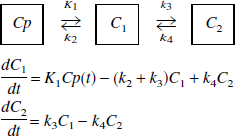
using measured plasma input functions, Cp(t). The radioactivity corresponding to a simulated region of interest (ROI) is given by C1 + C2. Two examples were used for these simulations which are similar to data from studies with RAC and MP and the plasma input functions were taken from actual PET studies. The model constants used for the RAC simulation data were K1 = 0.15 mL/min/mL, k2 = 0.36 min 1, k3 = 0.18 min−1, and k4 = 0.05 min−1 for a DV = 1.92 mL/mL. For the reference region simulations, a one-tissue compartment model was used with K1 = 0.08 mL/min/mL and k2 = 0.192 min−1. For the MP simulated data, K1 = 0.6 mL/min/mL, k2 = 0.06 min−1, k3 = 0.5 min−1, and k4 = 0.2 min−1 for a DV = 35.0 mL/mL For the reference tissue, the model parameters were K1 = 0.62 mL/min/mL and k2 = 0.062 min−1.
For comparison with the simulated data, human PET data from one RAC and one MP study were used. The PET scanner was a Siemens HR+, 63 slices, 4.5 × 4.5 × 2.4 mm full width half maximum (FWHM) in three-dimensional mode (see Wang et al. (2000) for experimental details using human subjects on the HR+). An arterial input function was measured for both tracers and plasma samples were analyzed for unchanged tracer (see Ding et al. (1997) and Volkow et al. (1993) for plasma sampling protocols). For the RAC study, 7.69 mCi was injected and 7.3 mCi was injected for the MP study. The scanning times were the same as used in the simulations. To increase the signal on each plane, contiguous planes were summed giving images with 4.8 mm FWHM. For both RAC and MP, one plane at the level of the basal ganglia was analyzed combining right and left. This gave a region containing 193 pixels for RAC and 237 pixels for MP. Data were analyzed both as the average of the pixels, which was taken to be the “true” value, and as the individual pixels.
There are a number of sources of noise in the PET image. The noise model used here is random, related to counting statistics. Noise is increased in the later time frames that have lower count rates because of radioactive decay. Taking into account scan times and the half-life of the isotope, the following formula was used to introduce random noise
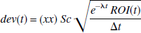
where ROI(t) is the original (noise free) simulated radioactivity (C1 + C2) at time t, e−λt ROI(t) refers to radioactivity not corrected for decay, eλt refers to the decay correction where λ is the half-life of the isotope which is either 110 or 20.4 minutes for the simulation of 18F or 11C. xx is a pseudo random number from a gaussian distribution with zero mean and variance of one, Sc is a scale factor that determines the level of noise, and Δt is the scan length. The simulated ROI with noise (ROIN) is given by

where ROI(t) corresponds to either RAC or MP and eλt dev(t) is the noise contribution at time t. The effect of introducing the decay factor is to take into account the difference in noise properties of the PET isotopes 11C and 18F with their different half-lives. Although the examples used here are both from 11C studies, this provides a mechanism for determining the effects of temporal differences in noise levels because the later scans of a 11C study will have significantly more noise relative to the earlier scans than an 18F study given the same scanning schedule. The amount of noise introduced in the simulations depends upon both the scale factor, Sc, and the half-life used in the decay factor. For the examples presented here, Sc ranged from 0.25 to 8. The average noise in the different sets of simulations is compared by
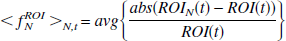
where ROI(t) is the original (“true”) data, ROIN(t) is the data with noise, and avg is the average over all time points (t) and over all data sets (N). A measure of how well the estimated ROI data approximates the original data is given by
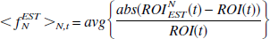
where ROINEST is the “smoothed” data set.
The scanning sequences used were the same as for the PET experiments. For RAC this was a total of 20 frames, 10 frames of 60 seconds and 10 frames of 300 seconds for 20 frames. For MP there were 22 frames, 10 × 60 seconds, 4 × 300 seconds, and 8 × 450 seconds. Data were analyzed graphically taking the average of slopes between 25, 30, to 75 and 25, 30, to 79 minutes for MP and 23, 28, to 53 and 23, 28, to 58 minutes for RAC. Region of interest estimates were determined using the one-tissue compartment fit for the entire time course and by the two part analysis. For the two part analysis, T1 was taken to be 10 minutes. However, to assure a smooth transition between the two regions, the fit to the first part was taken to be somewhat longer, 15 to 18 minutes, and the second part was begun at 8 minutes. The choice of 8 minutes insured a sufficient number of points in each region and also times for graphical analysis were all included in the second region. The DVs were redetermined using the smoothed data. Whether the estimated ROI data used for the analysis was from the two part or one part fit (the original Feng formulation) depended upon which gave the best fit to the (noisy) data set in a least squares sense. The DV was also determined by optimizing the model parameters for the two-compartment model for RAC and for the one-compartment model for MP. The starting parameters were taken to be the “true” values ± a random amount of 25% of the parameter value. The DV based on the optimized parameters is given by (K1/k2)(1 + k3/k4) for RAC and K1/k2 for MP. The one-compartment model was sufficient to recover the true distribution volume for the simulated MP data.
The DVR was also calculated using the reference region as described in Logan et al. (1996) and using the simplified reference model of Lammertsma et al. (1996) adapted to the linear iterative form of Eq. 5, which requires only an initial estimate of k2 designated
Solution of the differential equations and optimization of model parameters were accomplished using routines in Numerical Recipes in C (Press et al., 1988). Numerical integrations of the convolutions in Eqs. 2, 4, and 5 were performed using the routine “qtrap” also from Numerical Recipes in C (Press et al., 1988). A linear interpolation between time points was used for the ROI data. Equal weights were used in all of the linear analyzes.
RESULTS
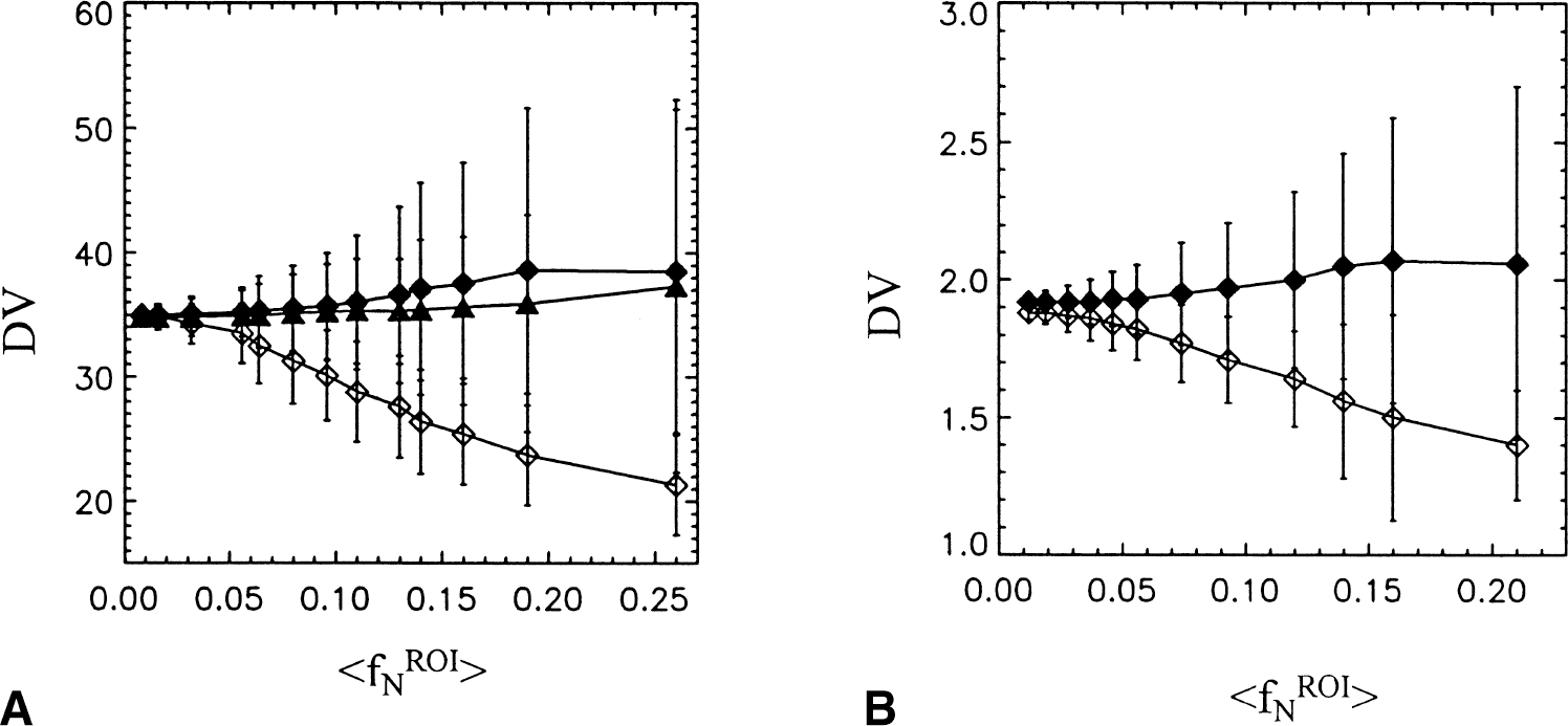
Results from the analyzes of the MP simulated data using the 11C and 18F factors in noise generation are given in Tables 1A and 1B, respectively. Plots are also shown of the mean and standard deviation of DVG, DVF, and DVFG for 11C in Fig. 1A. The average values over the 500 data sets of fNROI>t, <fNEST>t, the graphically determined DV, DVG, are reported as well as DVFG, which refers to the DV determined from the smoothed ROI data (ROIEST), whether by two part smoothing operation or from the one-compartment fit, whichever gave the best fit to ROIN. (At the higher noise levels this was generally the two part fit because of its greater flexibility.) Also given are DVF, the DV determined using the one-compartment solution of Eq. 2a (Feng's method), and DVNLS, determined from the model fit using the differential equations directly. The corresponding coefficients of variation (CV) reported as the standard deviation/mean are given in parentheses. As expected, DVG decreases with increasing noise. From Table 1A, (11C) DVG shows a 18% decrease in the mean as fNROI>N,t increases from 0.008 to 0.11. At the highest noise level tested (fNROI>N,t =0.26), the decrease in DVG was 40%. Similar results were observed by (Abi-Dargham et al., 2000) in simulations based on [11C]NNC 112. The DV generated using the 2 part fit (DVFG) shows an increase in average value with increasing noise, 10% over the true value at the highest noise level. Both DVF and DVNLS based on the one-compartment model gave the same results with a much smaller increase in both the DV and coefficient of variation. At intermediate noise levels (fNROI> = 0.10), DVFG, DVF, and DVNLS give similar results. For all methods, the CV increases with noise but the 2 part fit has a somewhat larger CV because of the increased flexibility of the fit. Also, at the highest noise levels, the GLLS method fails in some cases in the determination of the solution vector, θC . For Sc = 8, 35 out of 500 DV determinations were either out of range (<0 or >100) or failed to generate a solution θC . For the 18F decay factor (Table 1B), the average value for DVFG changes very little with increasing noise and the CV is smaller than that for 11C noise, basically the same as for DVF and DVNLS. The decrease in DVG with increasing noise is also less, a decrease of 11% with increase in fNROI>N,t from 0.023 to 0.14. When fNROI>N,t is on the order of 0.14, the CVs for the 11C simulations are 50% greater than those of the 18F simulations (0.23 and 0.09, respectively for DVFG). The ROI estimates, {ROINEST(t)}, generated by the smoothing technique provide a better approximation to the original data than do the noisy data sets, {ROIN(t)}, as measured by the ratio fNEST>Nt/(fNROI>Nt which is on the order of 0.4 to 0.5 for all noise levels in both simulations.
Distribution volumes for MP simulated data with “true” DV of 35 using 11C and 18F noise from Eq. 8 with Sc as shown
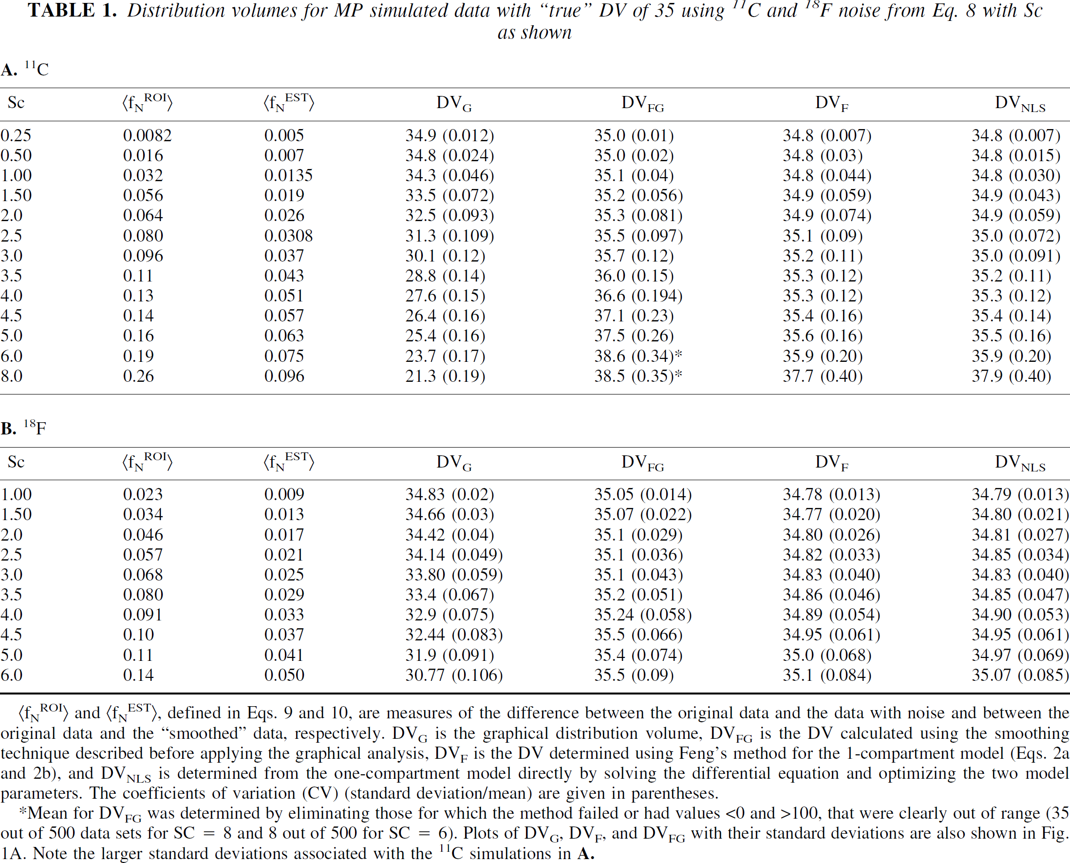
(fNROI) and (fNEST), defined in Eqs. 9 and 10, are measures of the difference between the original data and the data with noise and between the original data and the “smoothed” data, respectively. DVG is the graphical distribution volume, DVFG is the DV calculated using the smoothing technique described before applying the graphical analysis, DVF is the DV determined using Feng's method for the 1-compartment model (Eqs. 2a and 2b), and DVNLS is determined from the one-compartment model directly by solving the differential equation and optimizing the two model parameters. The coefficients of variation (CV) (standard deviation/mean) are given in parentheses.
Mean for DVFG was determined by eliminating those for which the method failed or had values <0 and >100, that were clearly out of range (35 out of 500 data sets for SC = 8 and 8 out of 500 for SC = 6). Plots of DVG, DVF, and DVFG with their standard deviations are also shown in Fig. 1A. Note the larger standard deviations associated with the 11C simulations in A.
Figure 2 (♦) illustrates simulated data (MP) generated with noise based on 11C. For these simulations fNROI>t = 0.10 and 0.095 for Fig. 2A and 2B, respectively. DVG was 43 and 30 mL/min/mL for Fig. 2A and 2B, respectively, whereas the smoothed data gave 44 and 35.9. The smoothed data in Fig. 2A differed from the “true” data significantly at later time points although still providing a good fit to the simulated data. In Fig. 2B, the smoothed data provides a good fit to the “true” data. Distribution volumes from the 1-compartment model (DVNLS) were 38.8 and 36.7 mL/mL.
Simulated time-activity data for example [11C]-d-threo-methylphenidate (MP). Original data (data without added noise) indicated by the solid line has distribution volume (DV) = 35 mL/min/mL. Data with noise added and 11C decay factor is indicated by ♦. The estimated region of interest (ROI) data is indicated by diam;. In both cases, the smoothed data appears to describe the noisy data but in A it differs from the “true” data.
Summaries of the data for RAC are given in Tables 2A and 2B. At the lowest noise level, the smoothing operation actually introduces more noise because fNEST>N,t is greater than fNROI>N,t (0.012 and .035, respectively). The RAC data indicate a 26% decrease from the true value in DVG for fNROI>N,t = 0.21, the highest noise level for 11C (Table 2A). For comparable noise levels, as measured by fNROI>N,t, DVG is 13% less for 11C and 6.4% less for 18F (Table 2B) (fNROI>N,t = 0.12). This indicates the greater sensitivity to noise in the later scans (because of 11C vs. 18F) as was also observed with MP. DVFG values from both sets of noise simulations show an increase with an increase in noise. The DVF in both cases underestimates the DV by approximately 10%. The CVs for all measures of DV increase with increasing noise. As with MP, the method fails more frequently as the noise increases. The DVNLS increases somewhat with increasing noise. To test the effect of varying the starting values of the model parameters, DVs were compared using both the true and the randomly displaced as initial values in the optimization procedure in the direct solution of the differential equations. For Sc = 2, there was a small improvement in using the “true” values, DVNLS = 1.93(0.08) mL/mL; but for Sc = 3.5, DVNLS = 1.99(0.22) mL/mL, the same as when the initial values were displaced from the true values.
Distribution volumes for RAC simulated data with “true” DV of 1.92 using 11C and 18F noise from Eq. 8 with Sc as shown
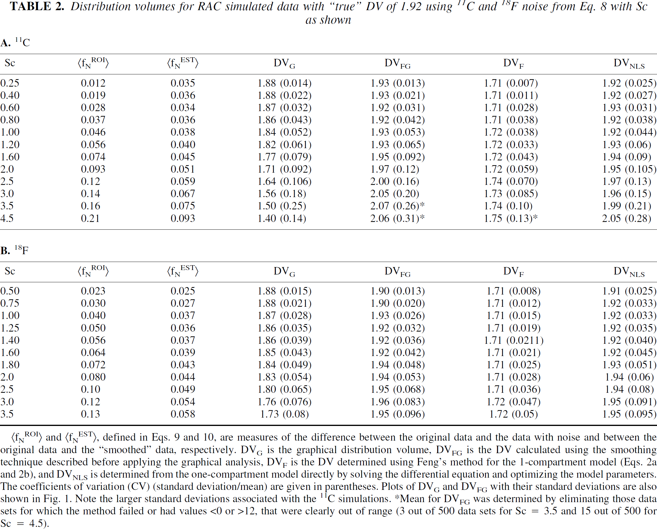
(fNROI) and (fNEST), defined in Eqs. 9 and 10, are measures of the difference between the original data and the data with noise and between the original data and the “smoothed” data, respectively. DVG is the graphical distribution volume, DVFG is the DV calculated using the smoothing technique described before applying the graphical analysis, DVF is the DV determined using Feng's method for the 1-compartment model (Eqs. 2a and 2b), and DVNLS is determined from the one-compartment model directly by solving the differential equation and optimizing the model parameters. The coefficients of variation (CV) (standard deviation/mean) are given in parentheses. Plots of DVG and DVFG with their standard deviations are also shown in Fig. 1. Note the larger standard deviations associated with the 11C simulations. *Mean for DVFG was determined by eliminating those data sets for which the method failed or had values <0 or >12, that were clearly out of range (3 out of 500 data sets for Sc = 3.5 and 15 out of 500 for Sc = 4.5).
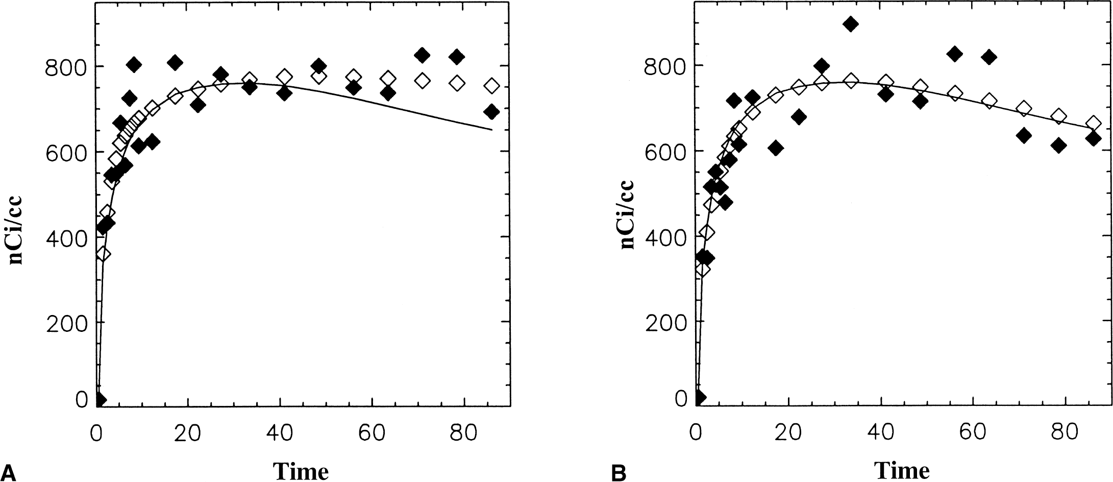
Figure 3 illustrates examples from RAC (♦) generated with noise based on 11C (fNROI>t = 0.10). In Fig. 3A, the smoothed data underestimates the “true” data and in Fig. 3B, the smoothed data is close to the “true” data. DVG is 1.58 (Fig. 3A) and 1.70 (Fig. 3B) mL/mL. The smoothed data (diam;) has fNEST>t = 0.051 (Fig. 3A) and 0.034 (Fig. 3B). DVFG = 1.74 (Fig. 3A) and 1.90 (Fig. 3B) mL/min/mL and DVNLS from the 2-compartment model was 1.73 (Fig. 3A) and 1.85 (Fig. 3B) mL/mL. DVF = 1.61 (Fig. 3A) and 1.71 (Fig. 3B) mL/mL.
Simulated time-activity data for example 11C raclopride (RAC). Original data (data without added noise) indicated by the solid line has DV = 1.92 mL/mL. Data with noise added and 11C decay factor is indicated by ♦. The estimated region of interest (ROI) data is indicated by ⋄. In both cases the smoothed data appears to describe the noisy data but in
Tables 3 and 4 present summaries of simulations of DVR calculations using reference tissue data. Average values over all 500 data sets of DVRG with the average k2 (K2 -REF ) (Logan et al., 1996), DVRFL calculated from the parameters of the simplified reference tissue model (Lammertsma and Hume, 1996), DVRFG calculated graphically using the smoothed data, and k2 -REF and DVRFG calculated graphically without k2 -REF . For MP, DVRFG calculated using the k2REF determined from the reference region and the “true” data was also reported (last column).
Distribution volume ratios for MP simulated data with “true” DVR of 3.5 using 11C noise from Eq. 8 with Sc as shown
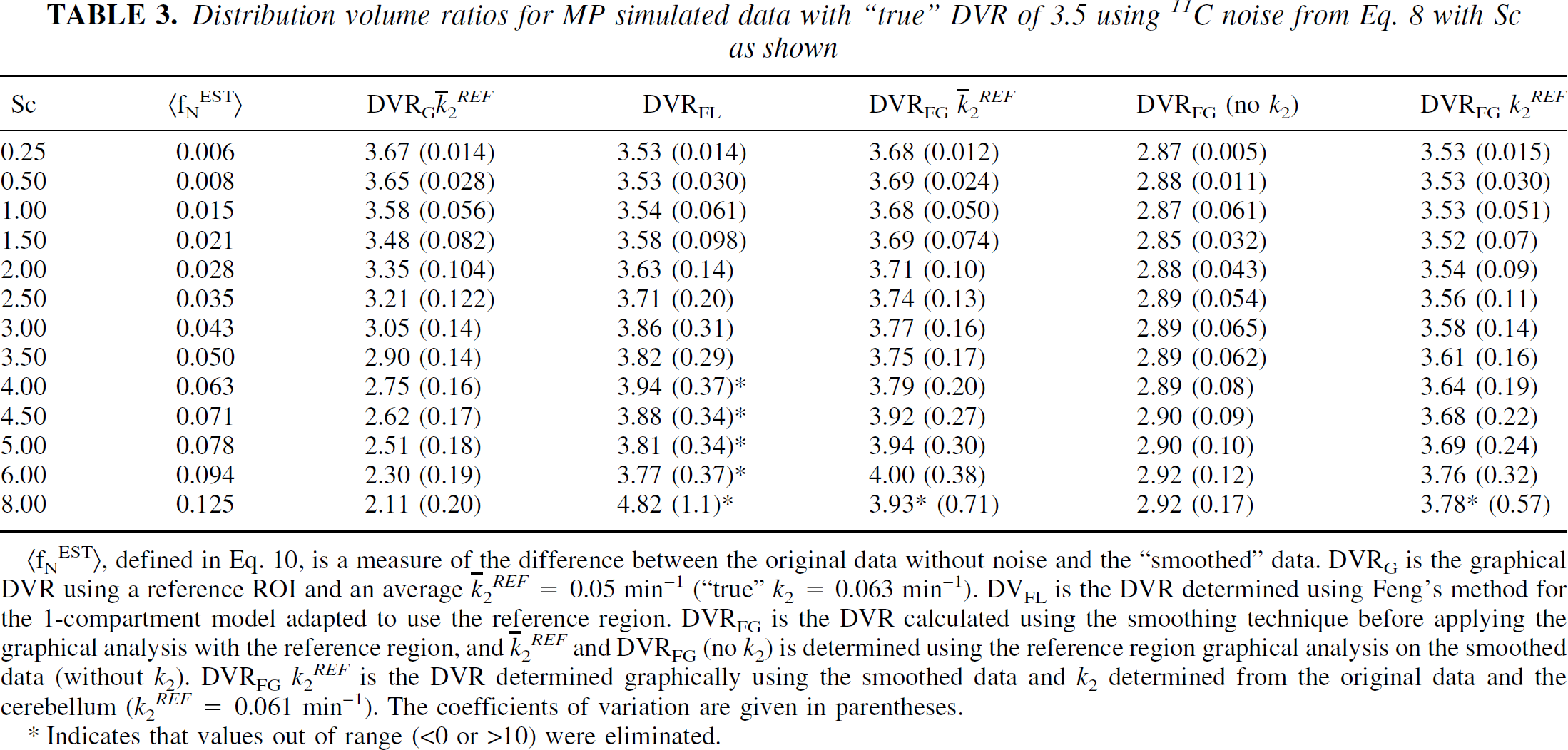
(fNEST), defined in Eq. 10, is a measure of the difference between the original data without noise and the “smoothed” data. DVRG is the graphical DVR using a reference ROI and an average
Indicates that values out of range (<0 or >10) were eliminated.
Distribution volume ratios for RAC simulated data with “true” DVR of 4.6 using 11C noise from Eq. 8 with Sc as shown
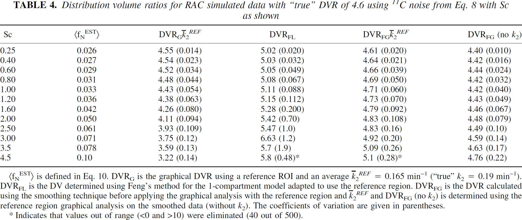
(fNEST> is defined in Eq. 10. DVRG is the graphical DVR using a reference ROI and an average
Indicates that values out of range (<0 and >10) were eliminated (40 out of 500).
For MP (Table 3), the DVRG is somewhat larger (5%) than the true value at the lowest noise level. This is because k2 -REF for the reference region differs from the actual k2 used in the simulations. For the same reason DVFG (k2 -REF ) also somewhat overestimates the DVR. DVRFL provides a good estimate at low noise levels, but the CVs increase more rapidly with noise than the other methods. At the highest noise levels, the means and CVs reported in Table 3 (*) were obtained by eliminating values <0 and >10 (approximately 7% of the values at the highest noise level). For MP, which conforms to a one-tissue compartment model, the linearized simplified reference tissue method does provide the correct value of k2 -REF (k2 -REF = 0.062 ± 0.017 for Sc = 3, and 0.064 ± 0.027 for Sc = 6). Using 0.062 for k2REF gives the results reported in the last column of Table 3. Although DVRFG (no k2) underestimates the DVR, the CVs are less and there is very little variation in mean from the lowest to highest noise level.
Besides
For RAC at the lowest noise level (Sc = 0.25, Table 4) all DVRs except DVRFL are within 5% of the true value. The means of DVRG, DVRFG (
Figures 4 and 5 illustrate data generated using the reference tissue method for MP and RAC. The solid line indicates the original data. The input data were taken to be the original ROI and reference region data to see how well the methods work without the effects of added noise. In Fig. 4, the fit generated using the linearized reference tissue method (⋄) reproduces the original data set very closely (DVR = 3.6 mL/mL). In Fig. 5, the ROI data generated using the 2 part fit described previously is indicated by ⋄ and the fit generated using the reference tissue method is indicated by ♦. The true DVR was 4.6 and the DVRFG generated graphically from the 2 part fit was 4.62. The DVR calculated from the model parameters using the reference tissue method was 5.05 mL/mL, however, the DVR calculated graphically using the ROI estimated by the reference tissue method was 4.82 mL/mL. For DVRFG, the average value of k2 (0.165 min−1) was used, although for this data neglecting k2 introduces only a small error.
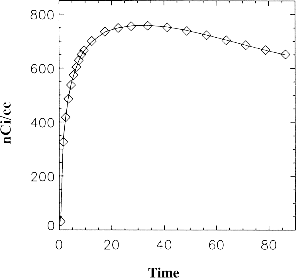
Data generated using the reference tissue method for [11C]-d-threo-methylphenidate (MP) (⋄) from Eq. 4. The original data is indicated by the solid line. The input data were taken to be the original region of interest data and reference region data without noise. The reference tissue method reproduces the original data.
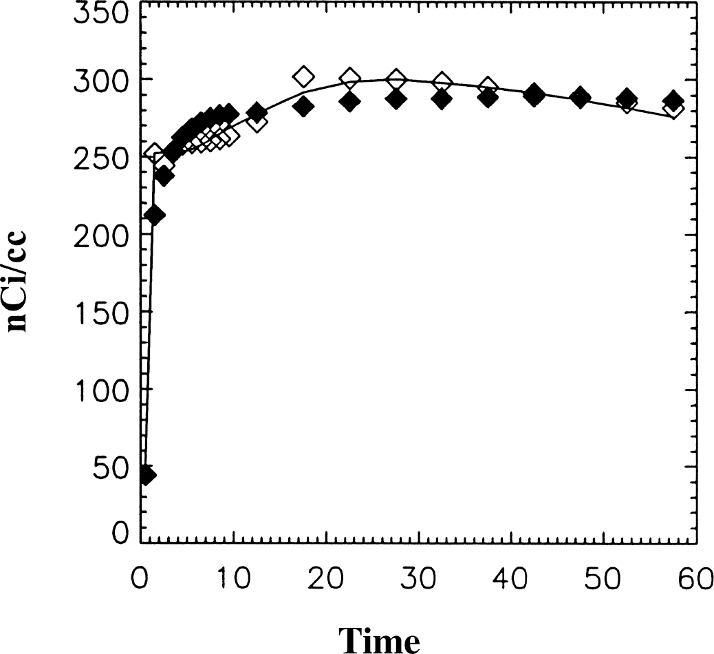
Data generated using the reference tissue method (without added noise) for 11C raclopride (RAC) (♦). The distribution volume ration (DVR) based on the calculated parameters was 5.05 from Eq. 6. The solid line is the original data that has DVR = 4.6. The region of interest (ROI) data indicated by ⋄ represent the estimated ROI fit using the two part fit with the reference region input. The DVR generated physically using this data was 4.66 using the average k2 and 4.5 without k2, both of which are very close to the true value and better estimates than the original reference tissue method.
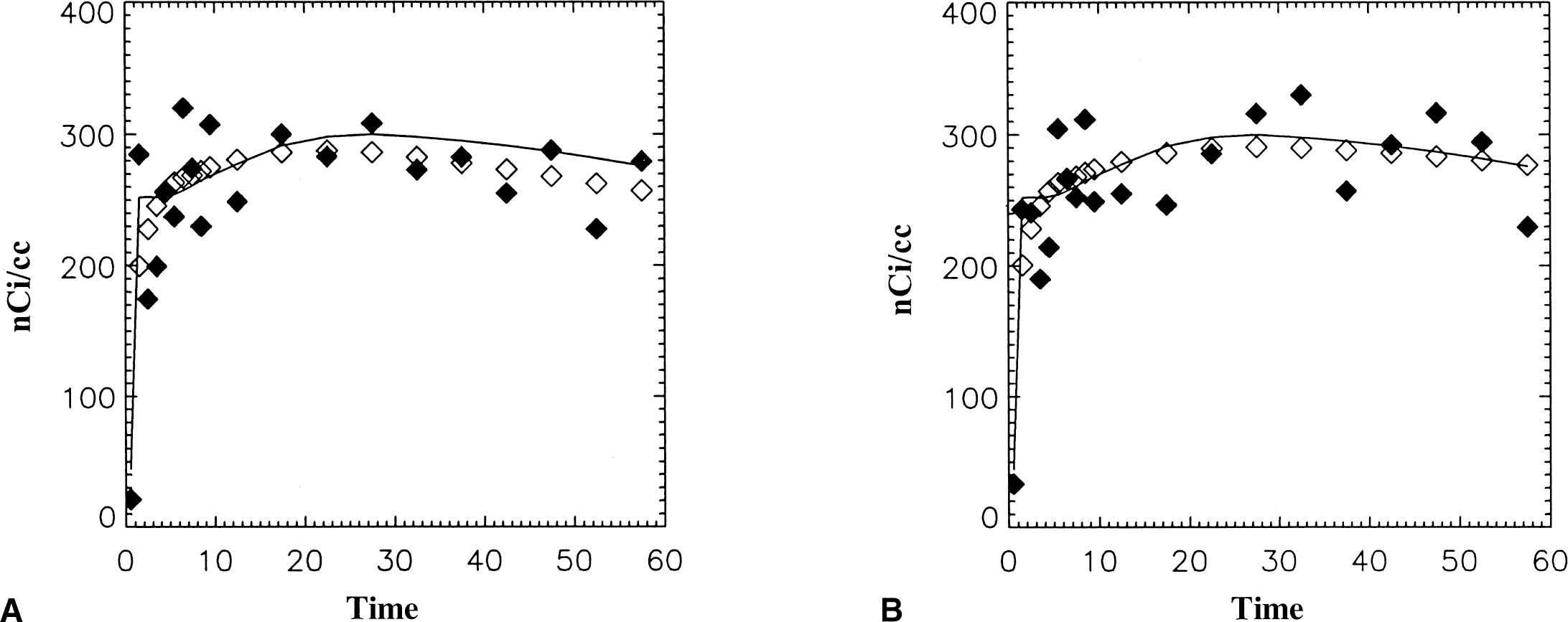
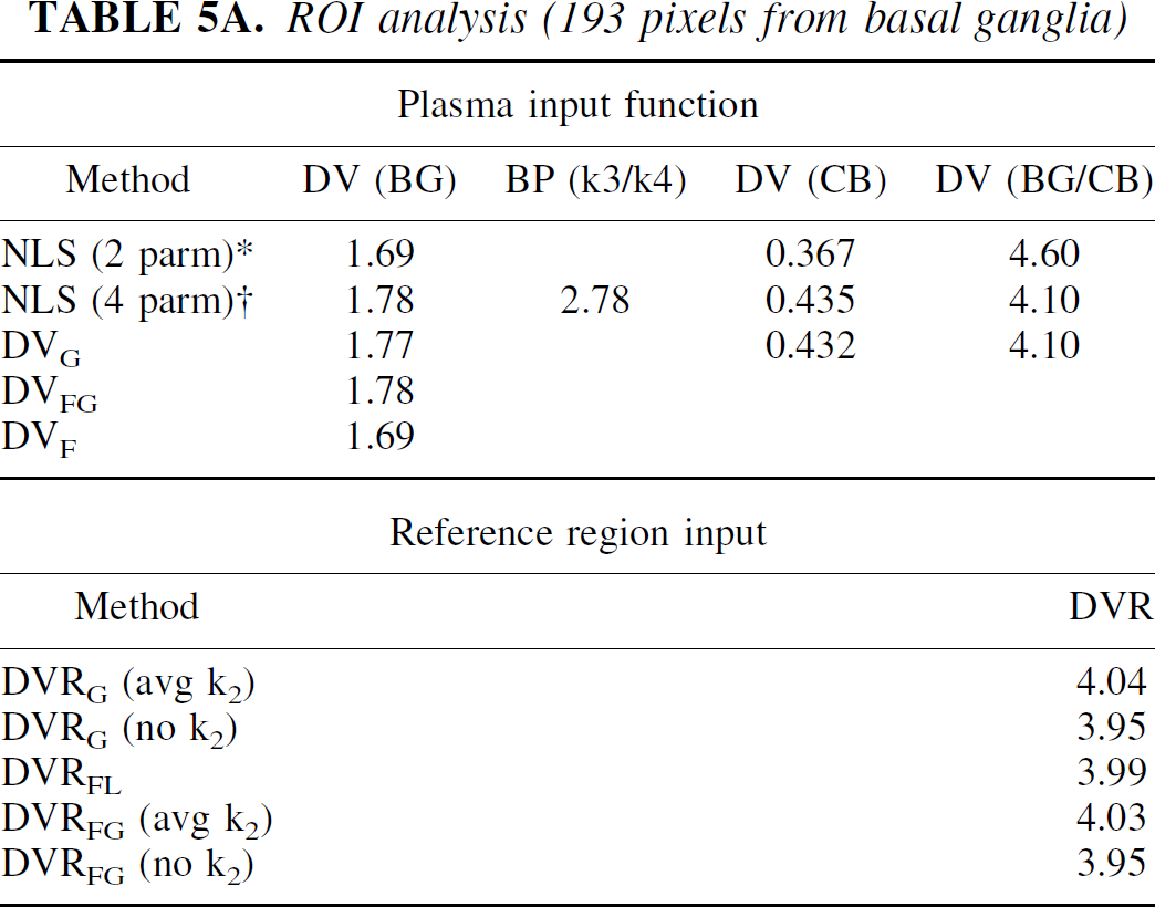
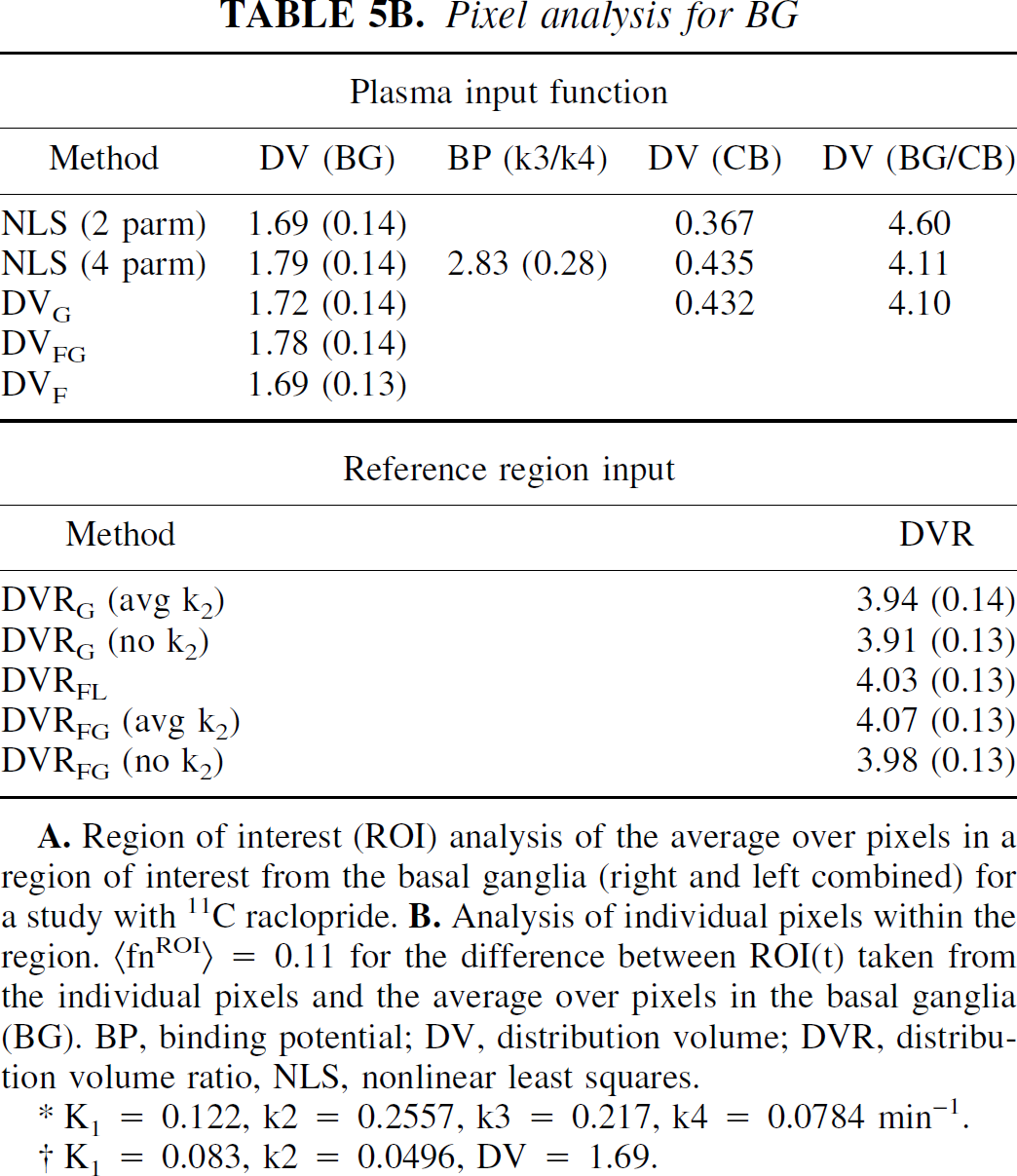
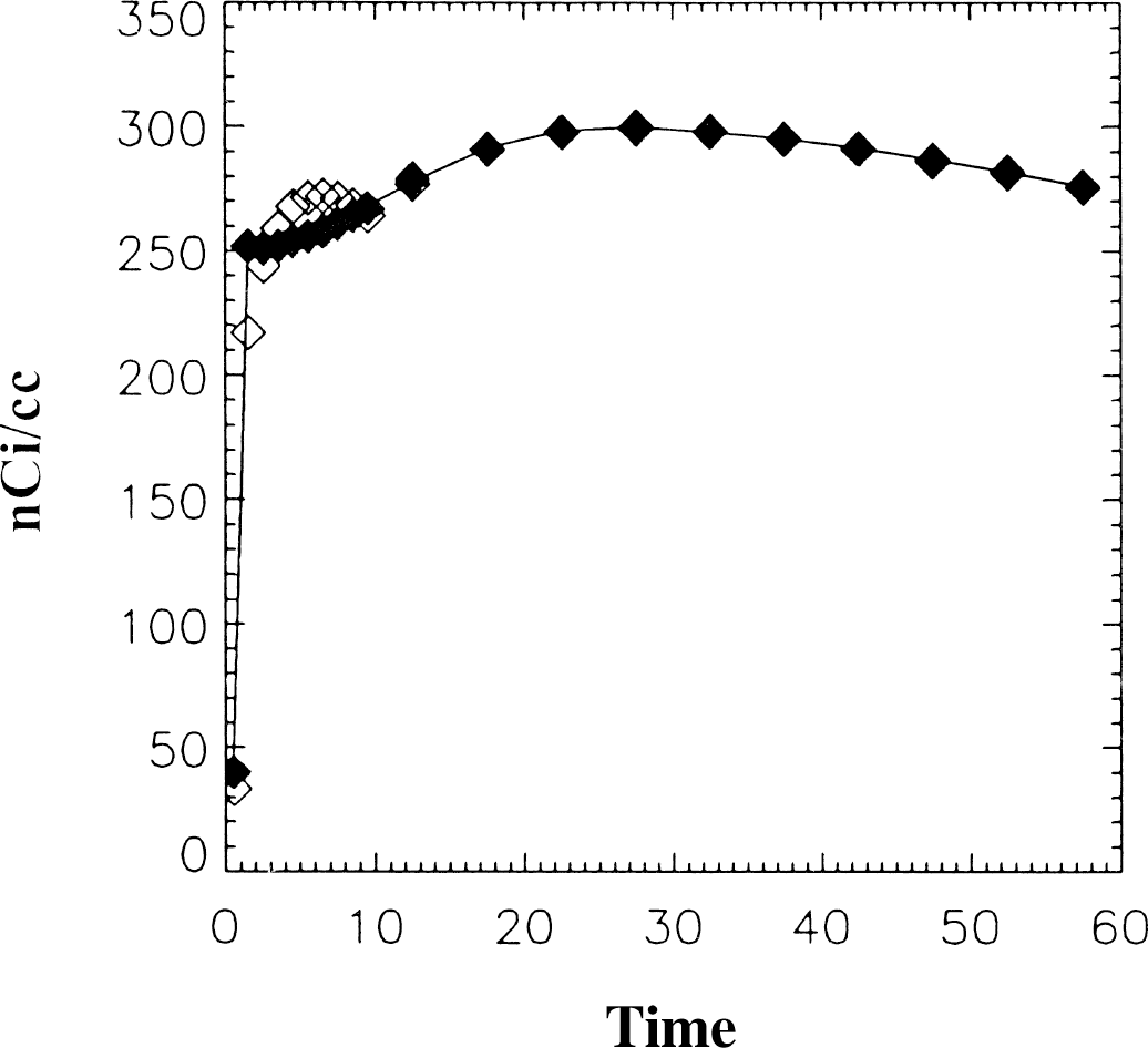
Table 5 presents the analysis of image data from a RAC study on the HR+. One hundred ninety-three pixels from one plane including right and left basal ganglia were used. In Table 5A, results from the ROI analysis of this data are given. Both 1- and 2-tissue compartment models were used to analyze the data from the basal ganglia (BG) and the cerebellum (CB), which was used as the reference region. For both regions, the two-tissue compartment gave a better fit to the data and agreed more closely with the graphical analysis. This was only a small difference in the BG, but the DV for the CB was 15% greater using the 2-compartment model. The binding potential (BP), defined as k3/k4, is 10% less than its estimation as DVR-1, using either the graphical or 2-compartment model for BG and CB DVs. Based on the 1-compartment model for CB, DVR-1 is 25% greater. The Feng method gave the same result as the NLS method for a one-compartment model. The DVR estimates were in close agreement for all methods. Results from the analysis of time-activity curves of the individual pixels are given in Table 5B. The average values of all methods were the same as for the ROI analysis except for DVG, which was 3% less. The binding potential, k3/k4, was in agreement with ROI analysis although with a CV of 0.28. The DVR data was also in good agreement with the ROI data. Although it is not possible to know the “true” data, using the average ROI data as a measure of the “true” data, fNROI> N,t was found to be 0.11. A plot of data from one pixel is shown in Fig. 6, with the image data indicated by ♦ and smoothed data is indicated by ⋄ with the solid line. The DVs from the various methods are in good agreement (within 6%).
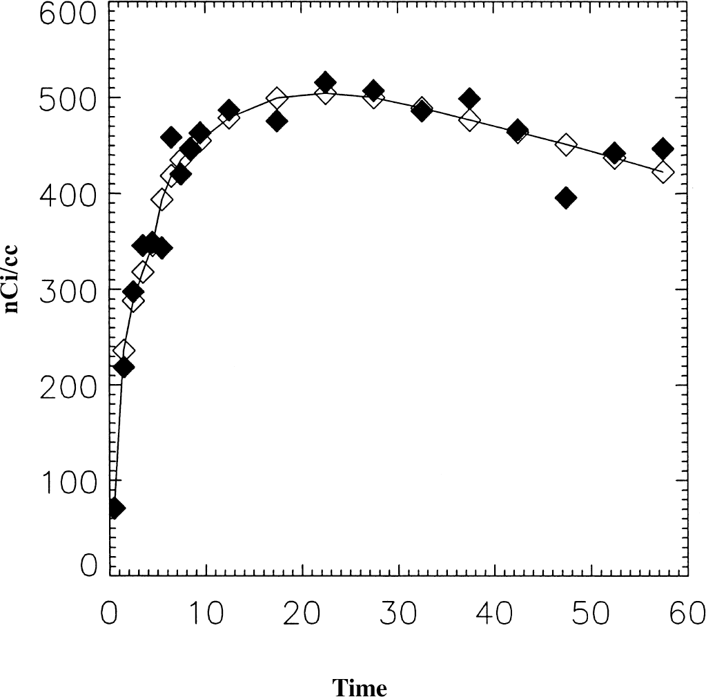
Data from a raclopride study representing one pixel at the level of the basal ganglia (♦). The smoothed data is indicated by ⋄. DVG = 1.8, DVFG = 1.91, DVF = 1.83, and DVNLS = 1.91 mL/mL.
ROI analysis (193 pixels from basal ganglia)
Pixel analysis for BG
K1 = 0.122, k2 = 0.2557, k3 = 0.217, k4 = 0.0784 min−1.
K1 = 0.083, k2 = 0.0496, DV = 1.69.
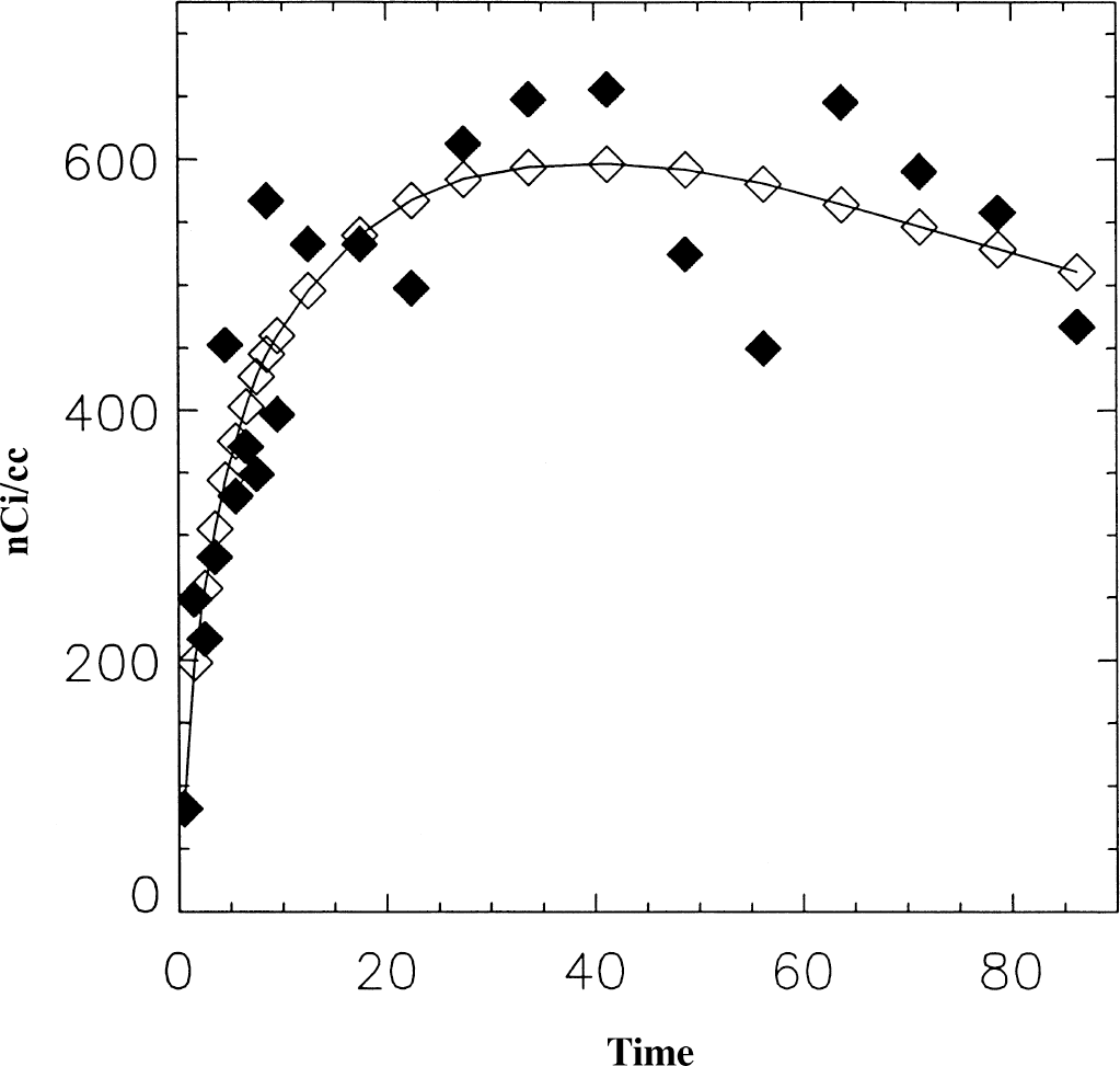
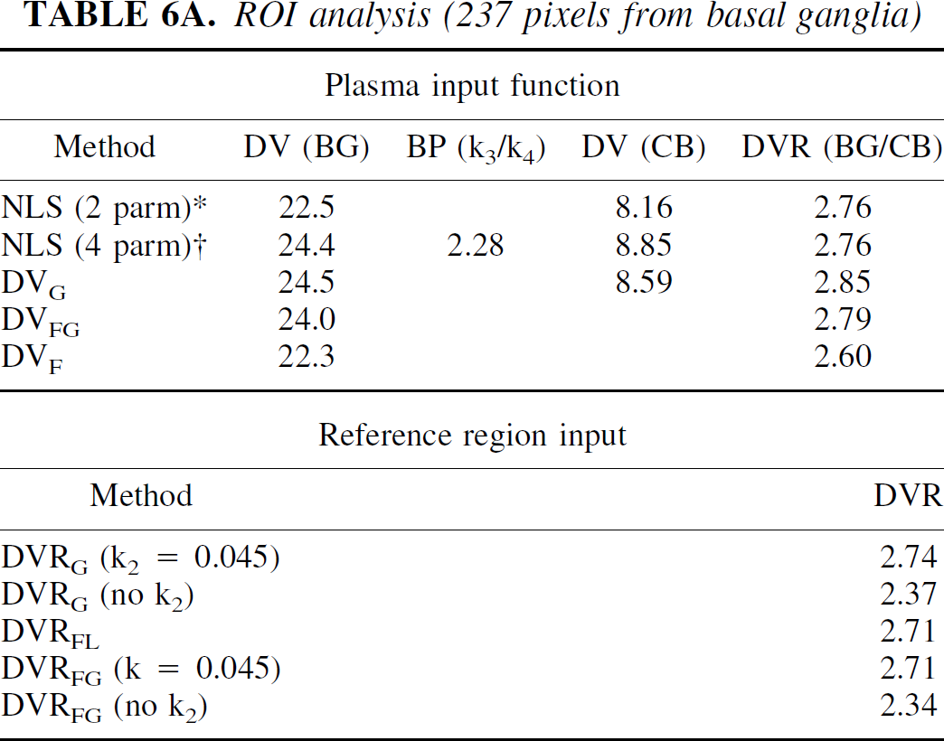
Table 6 presents the analysis of image data from a MP study on the HR+. Two hundred thirty-seven pixels from one plane including right and left basal ganglia were used. In this case, the image appears more noisy than the RAC study with fNROI> N,t = 0.18, also using the average time-activity curve as a measure of the “true” data. An example from this data set is shown in Fig. 7. In this example there was a small difference between DVs from the one- and two-compartment models for both BG and CB. The two-compartment model gave a slightly better fit to the data for the BG (the ratio of X2 for two-compartment to the one-compartment model was 0.64). This ratio was 0.10 for CB. DVG was closer to the 2-compartment value. Parameter values from the linearized reference tissue method were k2REF = 0.045, k2 = 0.02 min−1, and K1/K1REF = 1.19, which is in excellent agreement with values from 1-compartment model (NLS), 0.046, 0.019 min−1, and 1.16, respectively. In the pixel analysis, DVF agrees well with NLS (2 parm) (23.5 and 22.8 mL/mL, respectively), as expected because they both represent a 1-compartment model. Similarly, DVFG and NLS (4 parm) agree (25.1 and 25.6 mL/mL). The binding potential (k3/k4) calculated from the pixel analysis using the 2-compartment model has a large CV but is in reasonable agreement with DVR-1 based on DVFG or the DVR from the model solutions. The binding potential calculated from the ROI analysis is somewhat larger. DVG in the pixel analysis underestimates the DV by 20%. Similarly, DVRG in the pixel analysis underestimates the DVR, whereas in the ROI analysis, DVRG is in good agreement with the other methods. In the pixel analysis, DVRFG using k2 = 0.045 min−1 is close to the ROI values. Without k2, the DVRFG underestimates the DVR by 20%, assuming the “true” value to be 1.8. DVRFL is much more sensitive to noise with a large CV. This perhaps could be improved by using k2REF determined from the ROI analysis.
Data from a [11C]-d-threo-methylphenidate (MP) study representing one pixel at the level of the basal ganglia (♦). The smoothed data is indicated by ⋄. DVG = 20.4, DVFG = 26.7, DVF = 27.5, and DVNLS = 26 mL/mL.
ROI analysis (237 pixels from basal ganglia)
Pixel analysis for BG
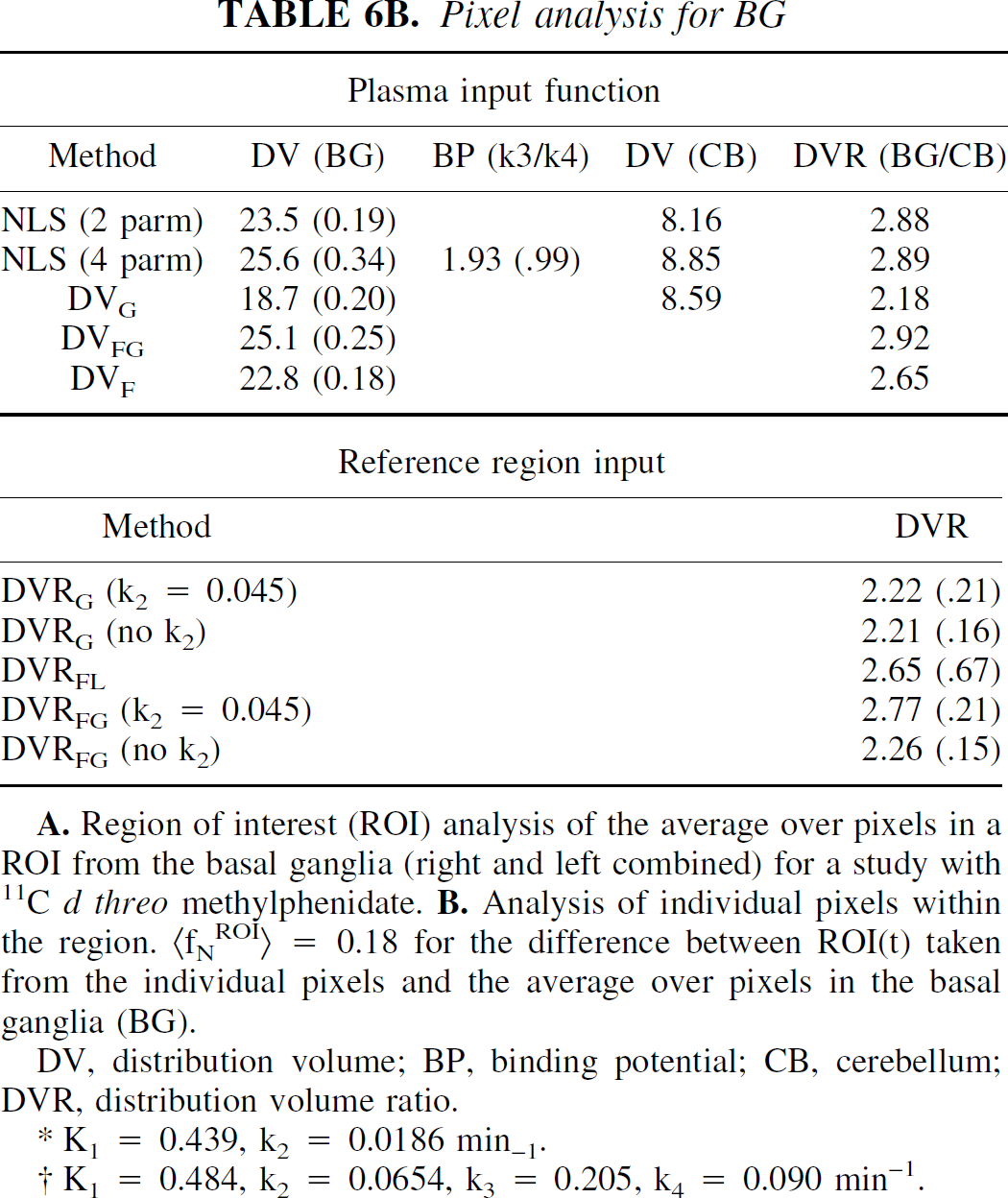
DV, distribution volume; BP, binding potential; CB, cerebellum; DVR, distribution volume ratio.
K1 = 0.439, k2 = 0.0186 min-1.
K1 = 0.484, k2 = 0.0654, k3 = 0.205, k4 = 0.090 min−1.
DISCUSSION
Graphical analysis of PET data has the advantage of being a rapid, easily applied method. In addition, it is model-independent and will yield the total distribution volume of a ROI whether it conforms to a 1-, 2-, or multi-tissue compartment model. However, the primary drawback is that it is subject to bias in the DV estimates when the time-activity data contain noise. This is less of a problem with small DVs and for ROI data; however, for the generation of DV images and in the case of noisy ROI data with higher DV values it would be useful to have a method that preserves the model-independent approach but estimates the total DV without a bias. To this end we have tested an adaptation of Feng's bias-free linear method for parameter estimation of the one-compartment model using simulation data based on the PET ligands, raclopride (DV = 1.92 mL/mL) and d-threo-methylphenidate (DV = 35 mL/mL), with varying amounts of noise. We also have performed some preliminary tests on image data using the same tracers for comparison. The kinetic parameters used in the simulations for these two ligands are very different illustrating two general examples. For MP, the binding constants, k3 = 0.5 and k4 = 0.2 min−1, are rapid and the large value of the DV is due to the slower tissue to plasma efflux, k2. In the other example (RAC), k2 is large (0.36 min−1) but the ligand receptor dissociation constant k4 in this example is considerably smaller (0.05 min−1). A result of these different kinds of kinetics is that a 2-compartment model is required to describe RAC, but an accurate measure of the total DV can be obtained from a 1-compartment model for MP. Why 1 set of parameters requires a 2-compartment model and the other does not has to do with the impulse response function of the 2-compartment model given by A1 exp(-α1t) + A2 exp(-α2t) (Carson et al., 1998), where A1,2 and α1,2 are combinations of K1, k2, k3, and k4,
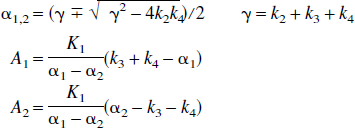
If one of the exponential terms dominate, a one-compartment model will adequately describe the data. Following (Carson et al., 1998) whether a two-compartment fit is required can be determined by considering the fraction of the area of the response function due to the second term for time T, that is
For RAC (simulated data), the ratio of Eq. 6 is 0.38 at 5 minutes, 0.168 at 20 minutes, 0.13 at 30 minutes, and 0.100 at 60 minutes. For MP (simulated data), the corresponding values are 0.017, 0.005, 0.0036, and 0.002. Therefore, MP appears as a one-compartment model, whereas RAC represents a two-compartment model.
For the image data (RAC), the ratios are 0.25, 0.10, and 0.085 for 5, 20 and 30 minutes and 0.078, 0.029, and 0.0208 for the same times for MP image data. The RAC image data still requires a 2-compartment model, but MP image data is not as clear as the simulation data and small differences between DVs are seen for the 1- and 2-compartment models. This introduces some ambiguity into what should be taken as the “true” value for the DV in this example. Also, attempts to estimate the BP directly are likely to be subject to large errors when the integrated response function ratios are small.
Because the RAC data requires a two-compartment model, the authors must verify that the method used here can in fact describe the two-compartment model. This is illustrated in Fig. 8. The solid line is the two-compartment solution to Eq. 7 and ⋄ represents the two part fit using Feng's one-compartment model. The two part fit differs slightly from the true model at early time points but is identical with the model at later times, which determine the DV. An “exact” fit to the model (indicated by ♦ in Fig. 8) can be obtained by including a third term in the smoothing operation of the first time interval so that Eq. 2a has an additional term on the righthand side consisting of Q exp(-
Data generated using the two part fit (without added noise) for 11C raclopride (RAC). ** indicates the fit using 3 parameters and ** indicates the fit using 2 parameters. The solid line is the original data. Distribution volumes were the same for both (1.91).
In many instances, data from RAC studies can be described by a one-compartment model, in which case the Feng method for a one-compartment model would be adequate. There are many cases in which little difference exists between the fits for a one- or two-compartment model (Koeppe et al., 1991; Carson et al., 1997). There are also instances in which the “nonspecific” reference regions are better described by a 2-compartment model. This has been observed for some studies with the radioligands 11C raclopride (for example, Logan, 2000) and 18F spiperone (Logan et al., 1987). Also, Abi-Dargham et al. (2000) observed that a two-compartment model gave a somewhat better fit to cerebellar data for the D1 ligand, [11C]NNC 112. In cases such as these this method would be applicable without the necessity of determining which model to apply.
Although values close to the original DV or DVR were recovered in the mean, there are large variances at the higher noise levels. Certainly some data sets have DVs that differ considerably from the mean (for example, Figs. 2A and 3A). Some difficulties are encountered with all methods in the presence of significant noise. This smoothing appears to do a good job in the intermediate range. Furthermore, the failure rate increases at high noise levels. When the data differ from the “true” signal, the noise even when random can introduce an apparent bias because of the finite number of measurements. By combining several data sets (as in an ROI) a value closer to the true value is obtained. In the case of the graphical analysis, the combining must be performed before the analysis to eliminate the noise and the bias. Also, the bias can be reduced by combining time frames.
The advantage of the linear methods, the graphical methods or the GLLS method of Feng, over that of the nonlinear least squares method is that they provide a considerable savings in computing time, which is especially important in constructing images because of the large numbers of pixels and multiple slices. The time required to generate solutions in the nonlinear approach is dependent upon how close the initial guess is to the best solution and how noisy the data is. The method proposed here is not as rapid as the graphical approach, but because it converges in one or two iterations it provides a considerable savings in time over NLS methods. The reference region method of Lammertsma and Hume (1996) and Gunn et al. (1997), implemented in the linear form of Feng, is also a rapid method that works well when data conform to a one-compartment model, as in the example MP. However, for the two-compartment example, RAC, it overestimates the DVR somewhat at low noise and the overestimate increases at higher noise levels with the CV becoming very large. Similar problems have been observed with the simplified reference tissue model when either the reference region or the receptor containing region cannot be described by a one-tissue compartment model, although use of the more general reference tissue model (Lammertsma et al., 1996) may not have these problems. In any case, the two part smoothing using the same simplified method followed by graphical analysis gives the original DVR. There is some susceptibility to noise at high noise levels resulting in larger CVs.
This method should be able to provide unbiased estimates of the DV (or DVR) for ROI data or images with intermediate noise levels. At high noise levels particularly with 11C tracers, the DV or DVR will be overestimated with a large CV. If a 1-tissue compartment model is appropriate, then the Feng analysis with a measured input function appears to work well even at higher noise levels. The DVR calculations using the smoothing without k2 provides estimates with the lowest CVs but can underestimate the DVR for ligands with slow efflux such as MP. This can be improved by extending the analysis times for the graphical analysis. For RAC, however, the DVR estimate without k2 is good even at the highest noise levels. The smoothing method does work well for the two examples of image data presented here. More extensive testing on images with different tracers and different DVs will be performed to establish limits of applicability. The difficulties of parameter estimation in the presence of significant noise are illustrated in Figs. 2A and 3A in which the smoothed data appears to provide a good description of the noisy data but does not provide accurate estimations of the DV.
The noise level in PET data is most frequently a problem for short-lived isotopes (such as 11C) at longer time periods because of radioactive decay. In this study, we investigated the feasibility of a combination of the GLLS and the graphical methods to provide a bias-free estimate of the DV. However, because these methods have significant CVs at high noise levels, it also would be desirable to reduce the noise through improved counting statistics for the generation of parametric images.