Sage Journals: Discover world-class research

Abstract

Monitoring of local oxygen pressure in brain white matter (tipo₂) and of local hemoglobin oxygen saturation (rSo₂) with near-infrared spectroscopy (NIRS) are increasingly employed techniques in neurosurgical intensive care units. Using frequency-based mathematical methods, the authors sought to ascertain whether both techniques contained similar information. Twelve patients treated in the intensive care unit were included (subarachnoid hemorrhage, n = 3; traumatic brain injury, n = 9). A tipo₂ probe and an NIRS sensor were positioned over the frontal lobe with the most pathologic changes on initial computed tomography scan. The authors calculated coherence of tipo₂ and rSo₂, its overall density distribution, its distribution per data set, and its time evolution. The authors identified a band of significantly correlated frequencies (from 0 to 1.3 × 10³ Hz) in more than 90% of the data sets for coherence and overall density distribution. Time evolution showed slow but marked changes of significant coherence. By means of spectral analysis the authors show that tipo₂ and rSo₂ signals contain similar information, albeit using completely different registration methodologies.

Keywords

Near-infrared spectroscopy (NIRS)Frequency analysis Multitaper analysis Modeling

Despite medical and technological advances in neurosurgical intensive care, severe traumatic brain injury and severe subarachnoid hemorrhage still carry a poor prognosis. Invasive monitoring of cerebral oxygenation has recently been proposed as a means for the detection and prevention of cerebral ischemia in comatose patients (Vinas et al., 1998). This is even more desirable, inasmuch as it is assumed that episodes of insufficient cerebral oxygenation enhance secondary brain damage (Purves, 1972). Thus several new continuous oxygen monitoring technologies, like the registration of regional brain tissue Po₂ (tipo₂) and the monitoring of regional oxygen saturation (rSo₂) with near-infrared spectroscopy (NIRS), have been brought into clinical practice in order to monitor cerebral oxygen metabolism.

Registration of the regional partial oxygen pressure (tipo₂) was clinically introduced in 1993 (Maas et al., 1993) and several reports (Dings et al., 1998; Kiening et al., 1996; Meixensberger et al., 1998) were published that proved the technical stability and the applicability of this device in daily clinical practice. Furthermore, some authors (Kiening et al., 1996) deduced a clinical usefulness and a prognostic value of this method, which could not, however, be verified by others (Vinas et al., 1998).

Reports about the usefulness of NIRS are contradictory as regards its technical reliability and clinical value (Büchner et al., 2000; Henson et al., 1998). Some of these studies report technical insufficiencies (Büchner et al., 2000; Kiening et al., 1996) of the measuring device itself; others question the results produced by the device, as being unrealistic for physiologic reasons (Schwartz et al., 1996). Other studies (Lewis et al., 1996), however, report useful and reasonable results with this methodology.

It is our opinion that both methods have potential for clinical application. Our goal, therefore, was to find a solution to these inconsistencies and contradictions. We approached the issue under the following assumption: tipo₂ and rSo₂ are dependent on the oxygen that is delivered to brain tissue. Thus, at least somehow, the signals must be related to each other and, to some extent, must present similar information, provided any of the two signals gives reasonable data. To be successful in our investigation, we should also be able to define and reconstruct a relevant and clinically meaningful part of each signal. We then could pursue the clinical usefulness of both methods based on these reconstructed curves. As a prerequisite all procedures used should be based on a sound mathematical basis.

Herein we report the first steps of our work, the frequency analysis of the tipo₂ and NIRS data, and an assessment of whether these two signals are related to each other.

MATERIALS AND METHODS

Patients and data monitoring

Twelve patients with closed traumatic brain injury (n = 9) and aneurysmal subarachnoid hemorrhage (n = 3) were included in the study prospectively. All patients were automatically ventilated and sedated through registration time. Eleven patients were male; 1 was female. Mean age was 34 years (range 18–76 years). The study was approved by the local ethics committee, and the relatives of the patients had given their informed consent. The treatment of these patients was performed according to the general guidelines used in the neurosurgical intensive care unit and was not influenced by the study.

A flexible polarographic Clark-type microcatheter (LICOX System; GMS mbh, Kiel, Germany) designed for continuous brain tipo₂ monitoring was inserted into frontal white matter. The catheter placement was guided by a specific introducer that was tightly fixed on a special skull screw. After insertion the catheter was firmly Luer-locked onto the introducer. The insertion depth of the probe was 34 mm (from dura level to catheter tip). Proper location of the catheter was ascertained using computed tomography scan. The measured tissue surface area was approximately 17 mm², and the data were output as partial oxygen pressure in mm Hg.

The cerebral oximeter sensors (INVOS 3100; Somanetics, Troy, MI, U.S.A.) consisted of one near-infrared light transmitter and two detectors (placed at a distance of 30 and 40 mm from the transmitter) housed within an adhesive strip. Near-infrared light at 730- and 810-nm wavelengths was used for maximum tissue penetration. It is postulated by the manufacturer that, using this sensor, near-infrared light is scattered by the tissues in two parabolic curves. The detector placed 30 mm from the transmitter receives light scattered predominantly from the scalp and skull, whereas the detector placed at 40 mm receives light scattered from the skull, scalp, and the brain tissue.

The distance of the two detectors allows intracranial penetration of more than 15 mm. The device measures a mixed venous–arterial oxygen saturation of the brain cortex based on hemoglobin saturation. Hereby 70% of the oxygen seen by the sensor originates from the venous compartment, 30% from the arterial compartment. This distribution is based on the assumption that cerebral vasculature has a greater volume of venous blood than arterial. The data are presented as rSo₂ index in arbitrary units (AU). The NIRS sensor was placed ipsilaterally to the tipo₂ probe on the patient's forehead and was secured with adhesive tape both to keep it fixed firmly in place and to achieve appropriate shielding from ambient light. We selected as registration site the frontal lobe with the most evident pathologic changes in primary computed tomography scan (otherwise, the right frontal lobe).

A multichannel digital-to-digital and analog-to-digital recording system was used for data storage. All patients were under camera observation during the registration period. The mean recording time was 4.5 days. Pertinent patient data and related information are shown in Table 1.

TABLE 1.

General clinical data

No.	Initials	Diagnosis	Age	Gender	Measuring time (hours)	No. of data points	No. of segments
1	E.B.	TBI	47	M	77	18,441	9
2	A.G.	TBI	18	F	43	10,245	5
3	W.H.	TBI	28	M	34	8,196	4
4	G.L.	TBI	63	M	102	24,588	12
5	A.P.	TBI	32	M	26	6,147	3
6	N.R.	TBI	27	M	9	2,049	1
7	O.R.	SAH	34	M	51	12,294	6
8	J.S.	SAH	43	M	17	4,098	2
9	J.S.	TBI	16	M	17	4,098	2
10	M.W.	TBI	76	M	26	6,147	3
11	Z.R.	SAH	32	M	17	4,098	2
12	Z.S.	TBI	36	M	17	4,098	2

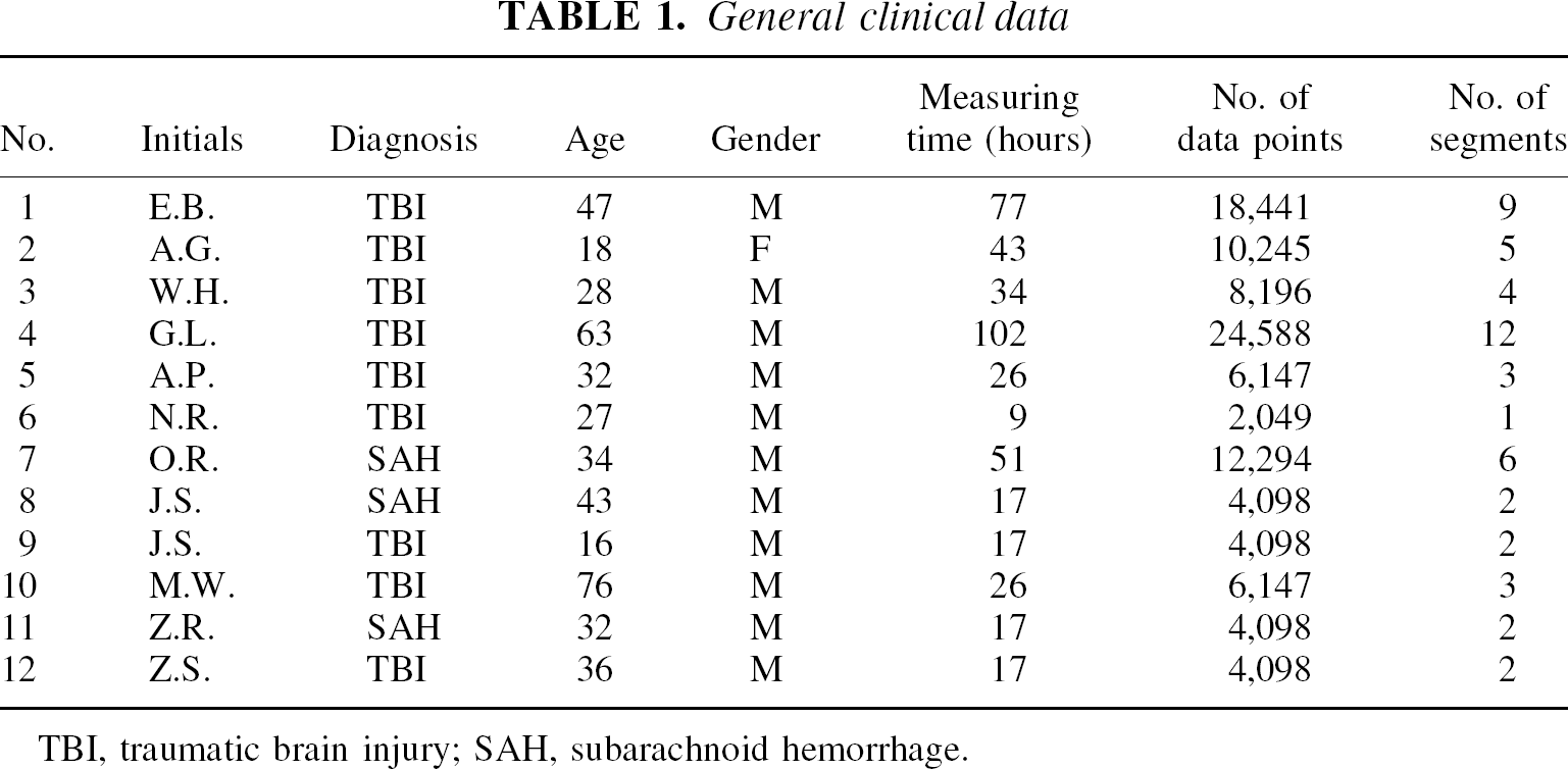
TBI, traumatic brain injury; SAH, subarachnoid hemorrhage.

Data preparation

All data were registered in 15-second intervals (0.07 Hz). First, we defined the time segments that were suitable for further analysis. We checked the quality limits, which were set by the manufacturers of the devices. We took into account only tipo₂ values above 15 mm Hg, because below that limit these data are technically unreliable (Lewis et al., 1996). Similarly, the rSo₂ data were limited to a range of 15 to 95 AU, according to the manufacturers' recommendations. We defined as obvious artifacts changes in absolute values with frequencies higher than the sample rate and spikes, which we could identify by camera observation as external disturbances. Such segments were also excluded. Furthermore, we made sure that the data of both devices had been recorded simultaneously, based on the internal computer clock of the devices.

Our next step was to split the remaining data sets of both signals in corresponding time-synchronized segments of 2,049 points, corresponding to approximately 8.5 hours each. This odd length was chosen for numerical reasons, to obtain optimal information by the algorithms used. However, we considered this interval to be long enough to contain relevant dynamical fluctuations. As a result we achieved 50 data sets comprising 427 hours of measuring time.

Data analysis

Mathematical methods. In principle all our analyses are based on the well-known mathematical lemma of Fourier, which states that every real-valued curve could be decomposed into sinusoidal waves without loss of information. The computational implementation for time series of this mathematical lemma is called fast-Fourier transformation (FFT). Usually the result of such a FFT is depicted as a so-called power spectrum, which shows the squared amplitude of each sinusoidal wave of the decomposition for each occurring frequency. Because of the finiteness of real-world time series the FFT often encounters difficulties, such as spectral leakage or sidelobing: part of the spectral information is lost for technical or computational reasons and the results, therefore, are adulterated. To overcome this problem, so-called window techniques have been introduced to minimize the loss of spectral information. An encouraging development on this sector it the multitaper method (MTM) established by Ghil and Yiou (1996). In contrast to standard window techniques that use only one fixed window, the MTM uses several different windowing functions—“tapers”—to calculate several spectral estimates S_k(f) of the real spectrum S(f), which is then a weighted sum of the different estimates. We found 5 × 3π tapers to be the best-suited choice of windowing for our data. Therefore, we always calculated five spectral estimates, where each estimate is smoothed by a special windowing function (i.e., a 3π taper or discrete prolate spheroidal sequence). The MTM spectrum is then obtained as:

S (f) = \sum_{k = 0}^{4} ω_{k} (f) S_{k} (f)

(1)

where ω_k(f) denotes a special weight for each estimate (Thompson, 1982). The method of choosing this weight is a theory on its own. In all of our calculations, we used a fully data-adaptive and recursive procedure that estimates bias and variance of each spectral estimate. These different estimates are calculated as:

S_{k} (f) = {(∣ \sum_{t = 0}^{n - 1} x (t) \frac{ν_{t, k} (n, W)}{a_{k}} e^{- i 2 π f (t - \frac{n - 1}{2})} ∣)}^{2}

(2)

where α_k is 1 for k even and the complex number i for k odd. n is the length of the dataset and v_t,k(n,W) denotes the k^th 3π taper. The window width of this taper is specified by the variable W, which in our case—due to the 3π taper—equals 3 xf_R, where f_R = 1/nΔt is the so-called Rayleigh frequency (with Δt denoting the sample interval of the data). This frequency specifies the lowest frequency resolvable by the FFT.

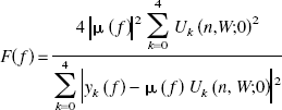
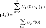
A second advantage of the MTM is a built-in statistical test, similar to the well-known F test, to check for the significance of each occurring frequency. Each figure in our work depicts lines pertaining to different levels of significance. This F variance–ratio test (Thompson, 1982) for the significance of line components can be constructed through the statistics F(f):

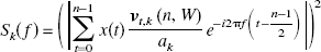
F (f) = \frac{4 ∣ μ (f) ∣^{2} \sum_{k = 0}^{4} U_{k} {(n, W; 0)}^{2}}{\sum_{k = 0}^{4} {∣ y_{k} (f) - μ (f) U_{k} (n, W; 0) ∣}^{2}}

(3)

In this formula the spectral estimates are represented by the function y_k(f), which is defined as:

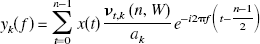
y_{k} (f) = \sum_{t = 0}^{n - 1} x (t) \frac{ν_{t, k} (n, W)}{a_{k}} e^{- i 2 π f (t - \frac{n - 1}{2})}

(4)

The real spectral estimates are therefore simply the absolute square of y_k(f):

S_{k} (f) = ∣ y_{k} (f) ∣^{2}

(5)

The function μ(f) is defined through the formula:

μ (f) = \frac{\sum_{k = 0}^{4} U_{k} (0) y_{k} (f)}{\sum_{k = 0}^{4} U_{k}^{2} (0)}

(6)

The function U_k(n,W;f - f₀) is defined as the FFT of v_t,k(n,W), which again means the k^th 3π taper. Thus the choice of the tapers has a direct influence on the statistical test (i.e., the significance of each occurring frequency).

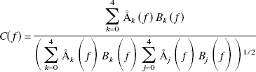
Based on these two mathematical concepts, we calculated the coherence or crosscorrelation of corresponding INVOS and LICOX data. The coherence is a well-known mathematical instrument for calculating the amount of common information enclosed by different time series. Because this method is also based on an FFT, it shows, for each frequency, whether the corresponding sinusoidal wave is a part of both time series and therefore common information. First, the MTM spectra of each single time series is obtained; the coherence is then calculated by the following formula, where we again used 5 × 3π tapers:

C (f) = \frac{\sum_{k = 0}^{4} Å_{k} (f) B_{k} (f)}{{(\sum_{k = 0}^{4} Å_{k} (f) B_{k} (f) \sum_{j = 0}^{4} Å_{j} (f) B_{j} (f))}^{1 / 2}}

(7)

where A_i and B_i denote the five different multitaper estimates of each time series and Å_i, B_i are their complex conjugates. To calculate the significance of the coherence amplitude a confidence test (Brillinger, 1981) similar to the F variance–ratio test was used. The coherence of each frequency was thereby compared to the coherence of two uncorrelated white noise signals (two purely random signals) and statistically evaluated. We always chose a significance level of 90%, denoting that for two purely random signals only ten percent of the frequencies need occur to be statistically significant.

Our first step was to find out whether the significantly coherent frequencies were concentrated in a specific frequency window or were scattered throughout the total spectrum. We counted how often each frequency occurred as significantly coherent through all the data sets. The resulting number for each frequency was normalized by division through the number of coherence computations (= data sets). Because we could identify a well-defined frequency band of high correlation, for our second step we calculated the percentage of significant coherent frequencies with significance greater than or equal to 90% within this band for each data set. The corresponding results were compared with the corresponding percentage of correlation of two uncoupled white noise signals. This procedure was necessary to make sure that within each single data set this frequency window was relevant and to exclude the possibility that the results of step one were merely the result of a summation over all data sets.

The third step was to evaluate the time course of the coherence through the total unsplit data set of each patient, enabling us to find exact time segments of high coherence and their duration. We therefore chose a window with a fixed length of 2,049 points and calculated the percentage of coherent frequencies according to the analysis of each data set. We then shifted the window by 4 points (corresponding to one minute) and did the same calculation again. This procedure was repeated until we reached the end of the patient's data set.

Finally, as a fourth step we reconstructed new curves by means of the significant frequencies to compare them to the original ones.

RESULTS

Step 1

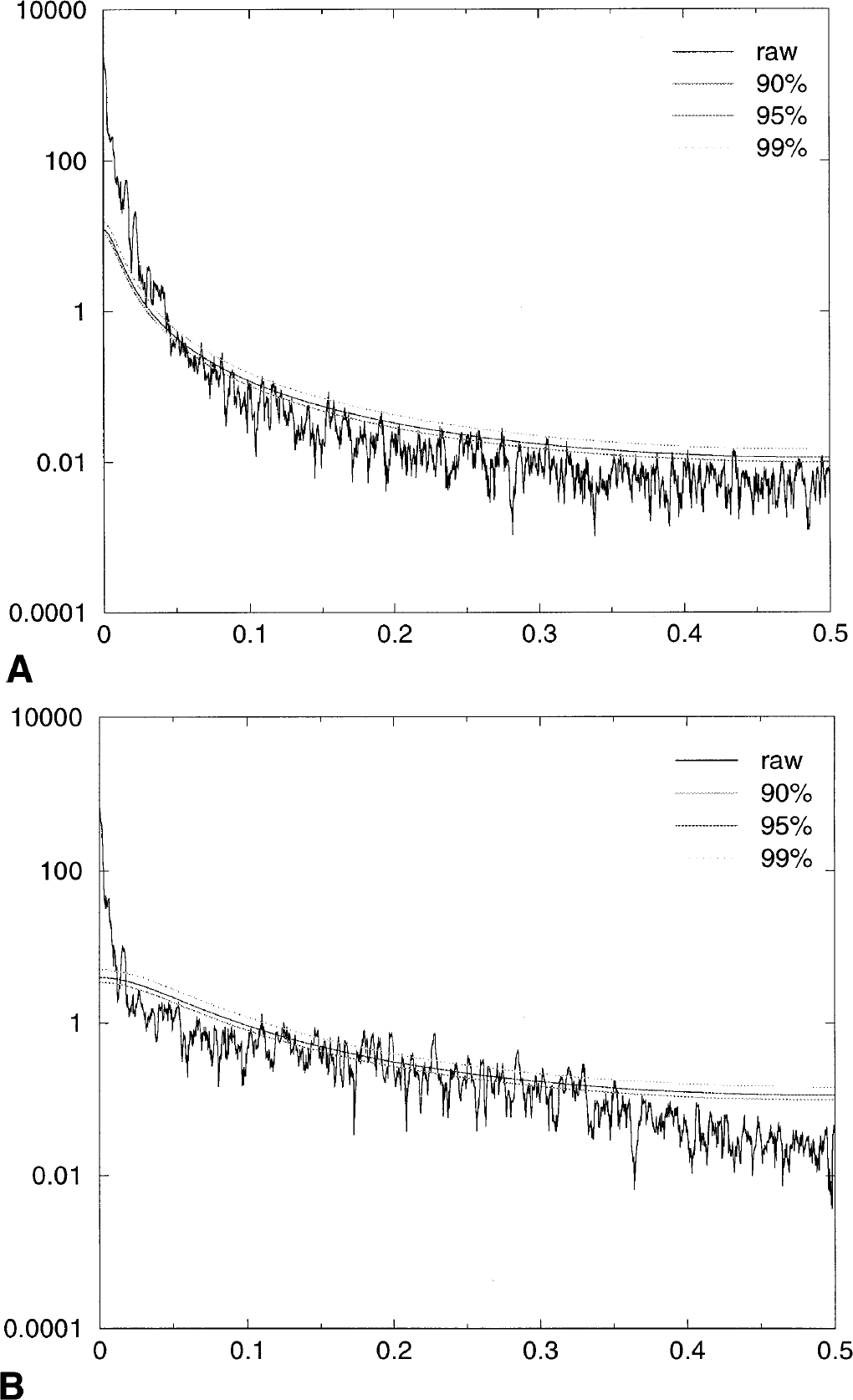
Figure 1 shows typical MTM spectra on which the coherence analysis is based. The tipo₂ spectrum (Fig. 1A) and the corresponding rSo₂ spectrum (Fig. 1B) show significant frequencies above the 90% limit, from 0 to 1.4 × 10⁻³ Hz. In the figures the significance levels of 90%, 95%, and 99% of statistical testing are given; many of the significant frequencies lie above 99%. Similar results can be seen for the coherence spectrum of the corresponding data sets. Again, significant coherence exists for lower frequencies (Fig. 2).

FIG. 1. (A)

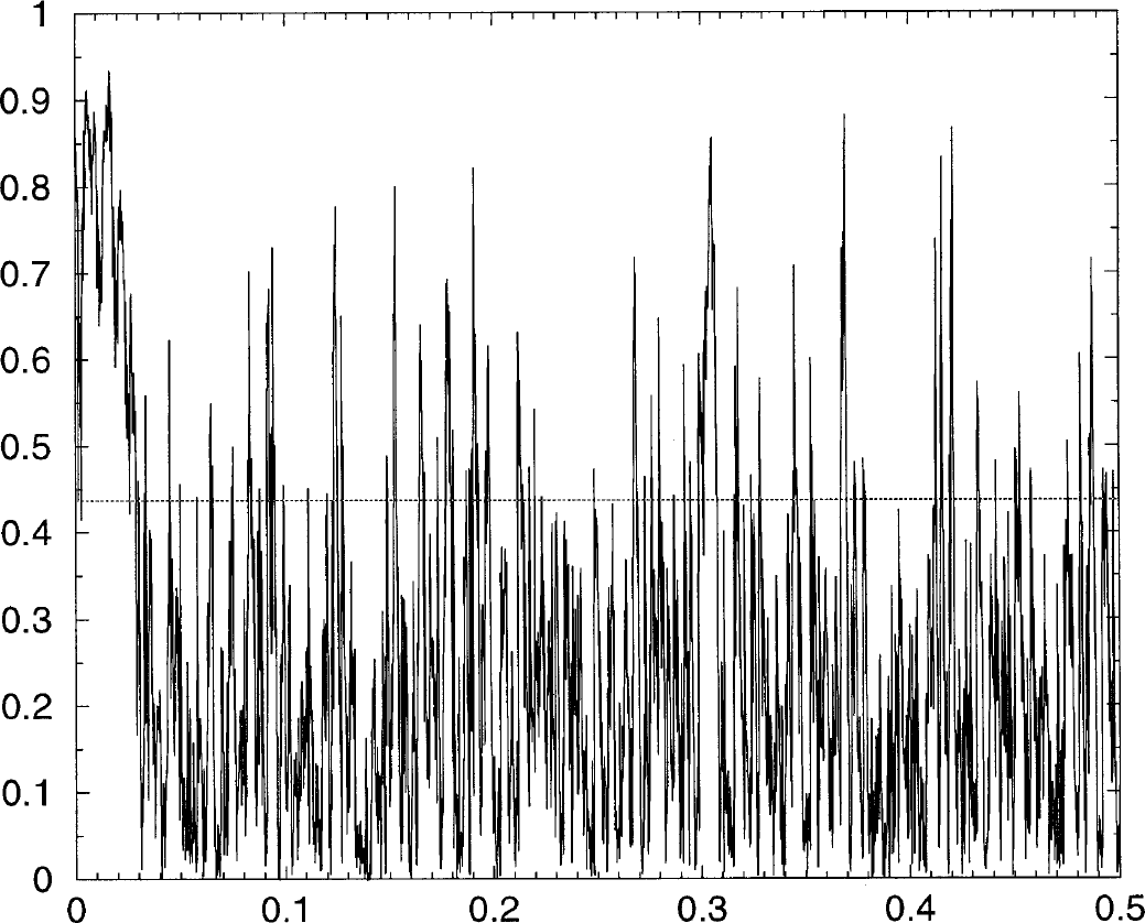
A typical multitaper method (MTM) spectrum of a tipo₂ data set. The x-ordinate shows the frequencies in units of the Rayleigh frequency (see Mathematical methods), whereas the y-ordinate represents the squared amplitude of each frequency in arbitrary units and is depicted in logarithmic notation. The respective significance levels of the statistical test used are presented as lines. (B) The MTM spectrum of the time corresponding rSo₂ data set is depicted in the same manner as Fig. 1A.

FIG. 2.

The coherence spectrum of both data sets of Figs. 1A and 1B. The x-axis represents the frequencies in units of the Rayleigh frequency; the y-axis shows the coherence of each occurring frequency, which is a unit-less number between 0 and 1. The horizontal line corresponds to the 90% significance level.

Figure 3 shows the normalized distribution of the significant frequencies summed up over all data sets. The line at 0.1 corresponds to pure white noise. We found a clear continuous peak in a frequency band from 0 to 1.4 × 10³ Hz, corresponding to a time resolution of maximally 12.5 minutes. This shows that most of the significant coherences are located within a well-defined frequency band and are not scattered through the total spectrum.

FIG. 3.

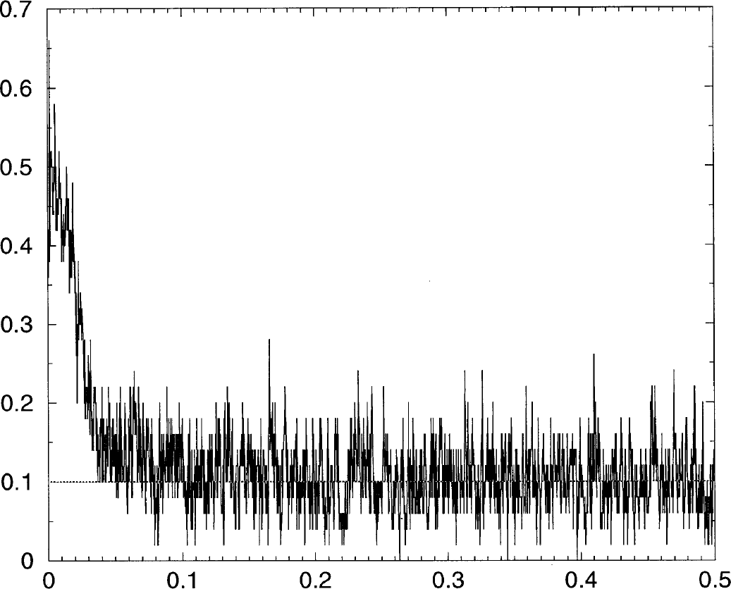
The distribution of significant coherent frequencies through all data sets. The x-axis represents the frequencies in units of the Rayleigh frequency; the y-ordinate represents the percentage of data sets with significant coherence for the particular frequency. The line at 0.1 belongs to the theoretical result for 2 uncorrelated white noise signals.

Step 2

Analysis within the single data sets yielded the result that 46 out of 50 sets had more significant coherent frequencies within this window as compared with uncoupled white noise signals (Fig. 4). This corresponds to 88% of all data sets.

FIG. 4.

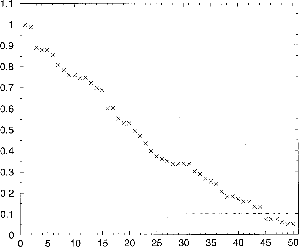
The percentage of the significant frequencies of each data set within the frequency band from 0 to 0.02 in units of the Rayleigh frequency. The x-axis represents each single data set denoted by a number; the y-axis, the percentage of significant frequencies. The horizontal line at 0.1 represents the theoretical result for uncorrelated white noise signals.

Step 3

We performed 23 windowed coherence computations through the total registration time of each patient. We observed time periods with a high coherence, which alternated with periods of low correlation (Fig. 5). We found, however, no clear time-dependent pattern behind those changes. We can therefore simply state this fact. Figure 5 shows a representative example of such a time evolution of coherence for patient 1.

FIG. 5.

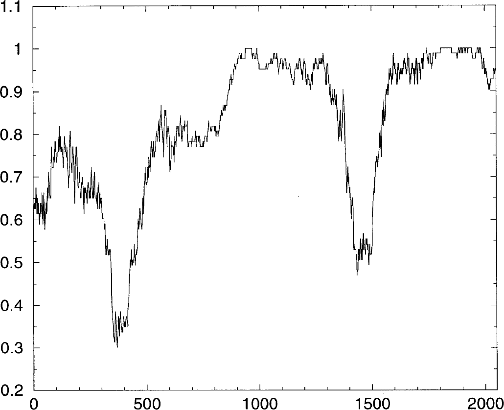
Windowed coherence of the complete data set of patient 5. The x-ordinate gives the number of time steps corresponding to the number of time-shifted coherence calculations that were done. The y-axis shows the percentage of significantly coherent frequencies within the defined frequency band of 0 to 0.02 for each window.

Step 4

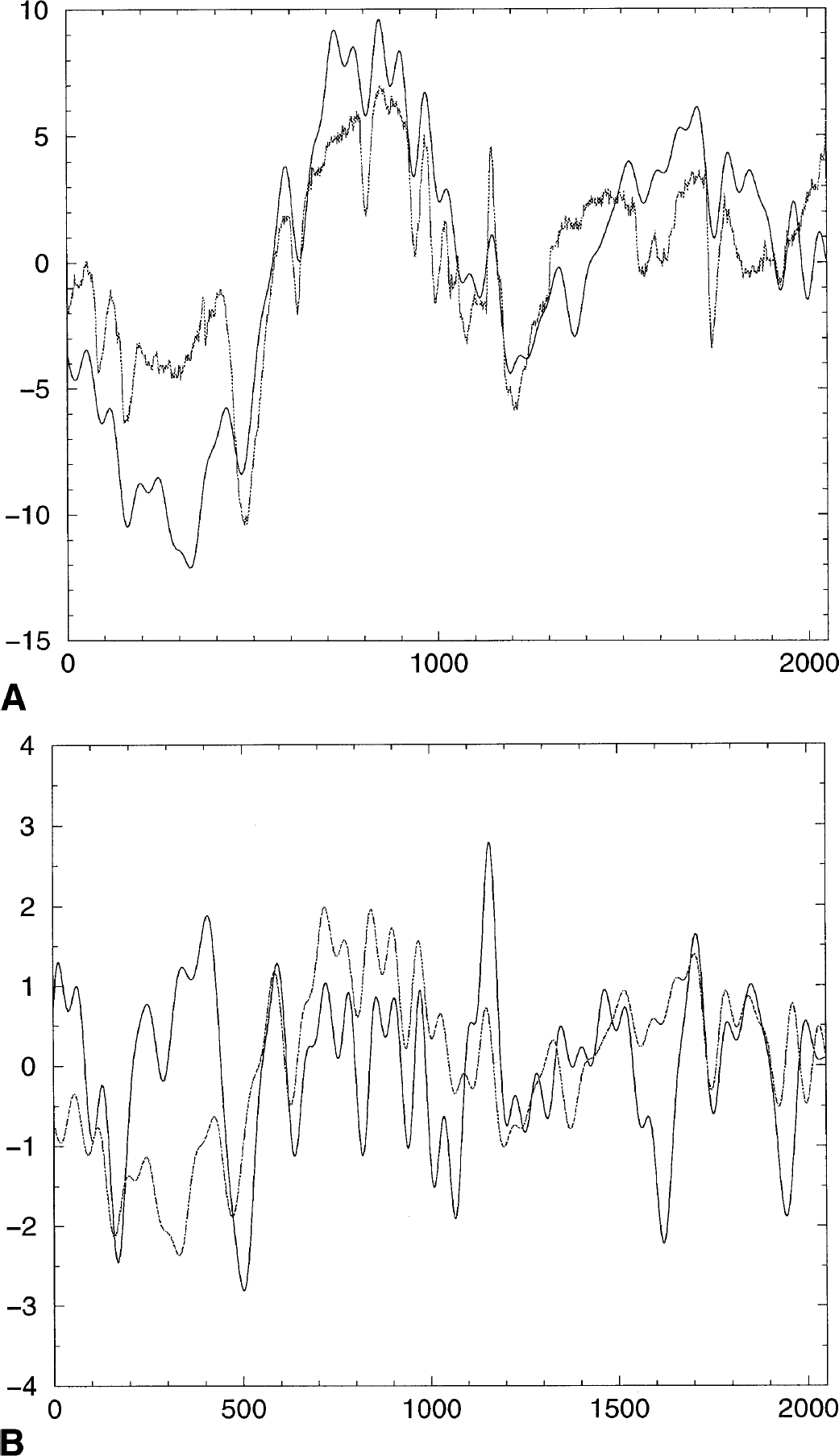
Using the significant frequencies within the identified frequency band we reconstructed both signals. Figure 6A shows an original and reconstructed tipo₂ curve, and Fig. 6B shows an example of reconstructed tipo₂ and rSo₂ curves. One can clearly see that the higher frequencies are cut off and that the main course of the signal is well represented.

FIG. 6. (A)

The original tipo₂ curve (solid line) and its reconstruction (dashed line). The x-ordinate represents the number of used data points; the y-ordinate shows the value of the tipo₂ measurement. For mathematical reasons the mean value of the tipo₂ measurement is subtracted from the data sets. (B) Reconstructions of a tipo₂ data set (dashed line) and its time corresponding reconstruction of the rSo₂ data (solid line).

DISCUSSION

The MTM used here provides a novel means for spectral estimation (Thompson, 1982) and signal reconstruction (Park et al., 1987) of a data set that is believed to exhibit a spectrum containing both continuous and singular components. The MTM analysis is therefore able to detect low-amplitude harmonic oscillations in a relatively short and noisy data set with a high degree of statistical significance. Provided enough background information about the data under analysis is present, more meaningful information about harmonic, anharmonic, and quasiperiodic elements and background noise of the data can be deduced. This method has been widely applied to problems in geophysical signal analysis, in which data are short and noisy. Because our data showed comparable properties we chose this methodology.

Our results demonstrate a significant correlation between tipo₂ and rSo₂ data within a frequency band of 0 to 1.4 × 10⁻³ Hz. These findings have several implications. From a mathematical perspective we can state that tipo₂ and rSo₂ contain similar information there. It is thereby important to note that the primary selection of the relevant frequencies was achieved purely by a mathematical analysis based on statistical testing. This was our primary and only criterion and no clinical considerations were taken into account.

There are several other points that have the potential to underline the validity of our results. The use of only a part of the total coherence frequency spectrum emphasizes the reasonability of our findings, because it is rather unlikely that two methodologies measuring different parameters at different locations should have an absolutely identical frequency spectrum. Furthermore, we had introduced an additional criterion for significance besides mathematical testing versus white noise: the significant frequencies should not be single peaks but rather a broad band. This implies stability and precludes spurious results, which can occur despite statistics. In our study the significant coherence is located over a broad frequency band (Fig. 2). We did not take into account single significant peaks in this study, despite possible relevance. Similarly, our results seemed realistic because, in the windowed analysis (Fig. 5), the significantly coherent periods were longer lasting events. These again represent more stable conditions of the system and, therefore, have a higher probability. A fast switching of coherence to noncoherence and vice versa and a short duration of each condition would make us more suspicious in terms of stability of our findings. In general, of course, we want to emphasize that a higher time resolution of the monitoring devices could give additional insights and further relevant information for the faster frequencies.

The discussion about the reliability of the NIRS methodology as applied in our study can be answered in a positive manner. Our analysis shows that the rSo₂ data seem to be meaningful in comparison to tipo₂ data, provided tipo₂ itself yields useful information. We state this with confidence because tipo₂ registration is a methodology that has been used for more than 40 years (Purves, 1972) and has been recently tested extensively in various studies (Kiening et al., 1996; Meixensberger et al., 1998) with the new intracranial probes.

One general prerequisite, however, is the careful application of NIRS technology. In our study we applied the NIRS sensor according to the manufacturer's prescription, without, however, any further specific measures. In addition, we had to check overall data quality before further evaluation. This is, however, a necessary precaution for every long-time registration procedure of data of any kind.

From a physiologic point of view both methods are able to reflect similar dynamical changes of cerebral oxygen metabolism within the selected time resolution. The assumption that tipo₂ and NIRS probes are measuring completely different aspects of oxygen metabolism in patients in neurosurgical intensive care cannot be supported by our data. Instead, they yield comparable information, and it is therefore reasonable to explore the correlation of tissue tipo₂ and rSo₂ data further. This reasoning is justified further under the following physiologic premises: NIRS measures the oxygen saturation of hemoglobin in brain grey matter. It is strictly related to the vascular bed with a relation of arterial to venous hemoglobin of 30% to 70% (Henson et al., 1998). In detail blood pressure, lung function, cardiac output, and autoregulation of cerebral vessels (blood volume) play a significant part in the regulation of this parameter, as well as brain metabolism. Furthermore, the freely soluble oxygen in the blood serum must be taken into account. This oxygen is dependent on the Fio₂ and is regulated by the partial pressure equilibrium between blood and air in the lungs. Tipo₂ data represent the partial pressure of O₂ in white brain matter and depend on all the parameters mentioned in the context of rSo₂ (Purves, 1972). In addition, we have to account for the diffusion of the oxygen from the vessels to white matter. This depends on the tissue properties and the length of the diffusion path. Thus, both parameters have quite a number of common physiologic dependencies that make our findings reasonable and that justify further studies.

We believe that our analysis could be a good starting point for future research in the field due to our discovery of several basic points: tipo₂ and NIRS seem to be related to each other. A meaningful curve of both parameters is available. This curve is reconstructed on purely mathematical grounds and all steps of curve analysis were based on statistical tests. No physiologic assumptions played a major role in the analysis and filtering of the data. The next, more interesting step now will be to correlate these curves to clinical events and to find physiologic explanations why or why not these two parameters correlate in specific situations.

References

Brillinger

B.R.

(1981) Time series, data analysis and theory. San Francisco: Holden-Day Press.

Büchner

Meixensberger

Dings

Roosen

(2000) Near infrared spectroscopy—not useful to monitor cerebral oxygenation after severe brain injury. Zentralbl Neurochir 61:69–73.

Dings

Meixensberger

Jager

Roosen

(1998) Clinical experience with 118 brain tissue oxygen partial pressure catheter probes. Neurosurgery 43:1082–1095.

Ghil

Yiou

(1996) Spectral methods: What they can and cannot do for climatic time series. In: Decade climate variability: dynamics and predictability ( Anderson

Willebrand

, eds), Amsterdam: Elsevier pp 445–448.

Henson

L.C.

Calalang

Temp

J.A.

Ward

D.S.

(1998) Accuracy of a cerebral oximeter in healthy volunteers under conditions of isocapnic hypoxia. Anesthesiology 88:58–65.

Kiening

K.L.

Unterberg

A.W.

Bardt

T.F.

Schneider

G.H.

Lanksch

W.R.

(1996) Monitoring of cerebral oxygenation in patients with severe head injuries: Brain tissue PO2 versus jugular vein oxygen saturation. J Neurosurg 85:751–757.

Kirkpatrick

P.J.

Smiclewski

Czosnyka

Menon

D.K.

Pickard

J.D.

(1995) Near-infrared spectroscopy use in patients with head injury. J Neurosurg 83:963–970.

Lewis

S.B.

Myburgh

J.A.

Thornton

E.L.

Reilly

P.L.

(1996) Cerebral oxygenation monitoring by near-infrared spectroscopy is not clinically useful in patients with severe closed-head injury: A comparison with jugular venous bulb oximetry. Crit Care Med 24:1334–1338.

Maas

A.I.R.

Fleckenstein

de Jong

D.A.

van Santbrink

H.M.

(1993) Monitoring cerebral oxygenation: Experimental studies and preliminary clinical results of continuous monitoring of cerebrospinal fluid and brain tissue oxygen tension Acta Neurochir 59(suppl):S50–57.

10.

Meixensberger

Jager

Dings

Baunach

Roosen

(1998) Multimodal hemodynamic neuromonitoring—quality and consequences for therapy of severely head injured patients. Acta Neurochir Suppl (Wien) 71:260–262.

11.

Metz

Holzschuh

Bein

Woertgen

Rothoerl

Kallenbach

Taeger

Brawanski

(1998) Monitoring of cerebral oxygen metabolism in the jugular bulb: Reliability of unilateral measurements in severe headinjury. J Cereb Blood Flow Metab 18:332–343.

12.

Park

Lindberg

C.R.

Vernon

F.L.

III (1987) Multispectral analysis of high frequency seismograms. J Geophys Res 92:12675–12684.

13.

Purves

M.J.

(1972) The physiology of the cerebral circulation. Cambridge, UK: Cambridge University Press.

14.

Robertson

C.S.

Contant

C.F.

Gokaslan

Z.L.

Narayan

R.K.

Grossman

R.G.

(1992) Cerebral blood flow, arteriovenous oxygen difference, and outcome in head injured patients. J Neurol Neurosurg Psychiatry 55:594–603.

15.

Schreiber

(1997) Nonlinear time series analysis. In: Nonlinear time series analysis ( Kantz

Schreiber

, eds), Cambridge, UK: Cambridge University Press.

16.

Schwartz

Litscher

Kleinert

Jobstmann

(1996) Cerebral oximetry in dead subjects. J Neurosurg Anesthesiol 8:189–193.

17.

Thompson

D.J.

(1982) Spectrum estimation and harmonic analysis. IEEE Proc 70:1055–1056.

18.

Vinas

Verweij

B.H.

Muizelaar

J.P.

(1998) Invasive monitoring of cerebral oxygenation. Crit Rev Neurosurg 8:31–40.

Comparison of Near-Infrared Spectroscopy and Tissue Po 2 Time Series in Patients after Severe Head Injury and Aneurysmal Subarachnoid Hemorrhage

Abstract

Keywords

MATERIALS AND METHODS

Patients and data monitoring

Data preparation

Data analysis

RESULTS

Step 1

Step 2

Step 3

Step 4

DISCUSSION

References