Sage Journals: Discover world-class research

Abstract

Arborization pattern was studied in pial vascular networks by treating them as fractals. Rather than applying elaborate taxonomy assembled from measures from individual vessel segments and bifurcations arranged in their branching order, the authors' approach captured the structural details at once in high-resolution digital images processed for the skeleton of the networks. The pial networks appear random and at the same time having structural elements similar to each other when viewed at different scales—a property known as self-similarity revealed by the geometry of fractals. Fractal (capacity) dimension, D_cap, was calculated to evaluate the network's spatial complexity by the box counting method (BCM) and its variant, the extended counting method (XCM). Box counting method and XCM were subject to numerical testing on ideal fractals of known D. The authors found that precision of these fractal methods depends on the fractal character (branching, nonbranching) of the structure they evaluate. D_cap s (group mean ± SD) for the arterial and venous pial networks in the cat (n = 6) are 1.37 ± 0.04, 1.37 ± 0.02 by XCM, and 1.30 ± 0.04, 1.31 ± 0.03 by BCM, respectively. The arterial and venous systems thus appear to be developed according to the same fractal generation rule in the cat.

Keywords

Box counting method Digital image processing Extended counting method Fractal dimension Fractal geometry Pial vascular networks

Blood supply of the brain is provided by a richly arborized network of vessels running along its surface (within the pia mater) connecting a few large arteries of primary supply (aa. carotes internae and aa. vertebrales) to thousands of arteries approximately 40 to 100 μm in diameter perforating the brain cortex. Further intracortical ramifications give branches ultimately connecting with the capillary rete—a dense mesh of endothelial tubes—creating the primary site of exchange for the brain's cells. It is important to understand the design of transfer routes nature uses to interconnect the four inputs of the brain's vasculature to the innumerable perforating arteriolar segments of the pial networks feeding the intraparenchymal circulation, as well as that of the pial venular networks collecting flow from it. In contrast with other organs, a large segment of the brain's arteriolar and venular networks is developed outside the organ boundaries rendering themselves to relatively easy visualization. Hence, the goal of the current study was twofold: first, to elaborate digital video technology for high-definition documentation of the pial arterial and venous networks in the cat, and second, to characterize their geometrical design as captured in their fractal properties.

Previous structural descriptions of the pial vasculature (Bär, 1980, Duvernoy et al., 1981; Hudetz et al., 1987; Mchedlishvili and Kuridze, 1984) were based on the use of elaborate taxonomy by the Horsfield (Singhal et al., 1973) and the Strahler (Jiang et al., 1994; Strahler, 1957) classification. It is difficult if not impossible to compare individual networks or networks from different species in a simple, conclusive manner using these extensive data sets.

Instead, statistical variations in these data sets were used to characterize changes in the networks in response to influence by species, age, and level of oxygenation or arterial pressure. The taxonomical approach translates the complex geometry of the pial networks into an elaborate and extensive data set without attempting to identify the concept of design. In contrast, the fractal approach yields a single measure of structure, the fractal dimension by fitting the fractal model of design to the spatial data set.

Fractal methods seem to gain on influence in structural studies of the vascular system. They have been used in studies of the retina (Family et al., 1989; Landini et al., 1993), lungs (Gan et al., 1993; Jiang et al., 1994; Weibel, 1991), heart (Bassingthwaighte et al., 1990; van Beek et al., 1989), kidney (Xu et al., 1994), and chorioallantoid membrane of the chicken embryo (Kurz et al., 1998; Sandau and Kurz, 1996), in addition to discriminating normal from cancerous vascularization (Gazit et al., 1997). To the authors' knowledge, this is the first article to analyze the arborization in the pial system using fractal methods.

MATERIALS AND METHODS

Video imaging of the pial vasculature

Images of the pial vasculature were obtained in the cat. The associated experimental procedures were conducted according to the Guide for Care and Use of Laboratory Animals published by National Institutes of Health (NIH), and were approved by the NIH Fogarty International Center and the Regional Committee of Science and Research Ethics of the Semmelweis University of Medicine. Video imaging was performed in vivo in the cat as follows.

Cats (2.5 to 3.5 kg in weight) were anesthetized by alpha-chloralose (50 mg/kg body weight, intraperitoneal). Closed cranial window technique reported earlier (Eke et al., 1979) was used to visualize an area of 12 mm in diameter over the brain cortex on the right side over the suprasylvanian gyrus. The size of the video image of the pial network corresponded to an area of 8 × 6 mm positioned over the gyrus in such a way that sulci are not shown on these images. Bolus injection of isotonic saline into the ipsilateral lingual artery was used to identify the arterial and venous networks based on their respective mean transit times (Eke, 1983; Eke et al., 1979). Digital images of the arterial and venous networks under epi-illumination were taken at 589 nm at a 640 × 480 pixel @ 8 bit resolution.

Digital image processing

The NIH Image program was used on a Macintosh Quadra 660 AV computer (Apple Computer, Cupertino, CA, U.S.A.) to process the digitized video images for a single line trace of the pial networks. Each step of this procedure is shown in Fig. 1. The gradient in the raw image needed to be removed before skeletonizing. It is the combined effect of the epi-illumination geometry and slight curvature of the brain cortex that reduces the contrast of small branches in the center and periphery of the image. This was eliminated as follows. First, the raw image was subject to repeated (50×) smoothing, an equivalent to optical defocusing. The resulting image is deprived of definitions of the vascular features but retains the gradient in the intensity profile of the image background. Subtracting the defocused from the raw image resulted in a corrected image with equally enhanced contrast for most of the features of the pial vasculature, against an evenly “illuminated” background. Definition of these images was improved by manual tracing their laser prints, followed by scanning the images at 600 dots per inch resolution. In the final step, the resulting black and white bitmapped image was skeletonized to yield a one-pixel-wide trace of the network suitable for fractal analysis.

FIG. 1.

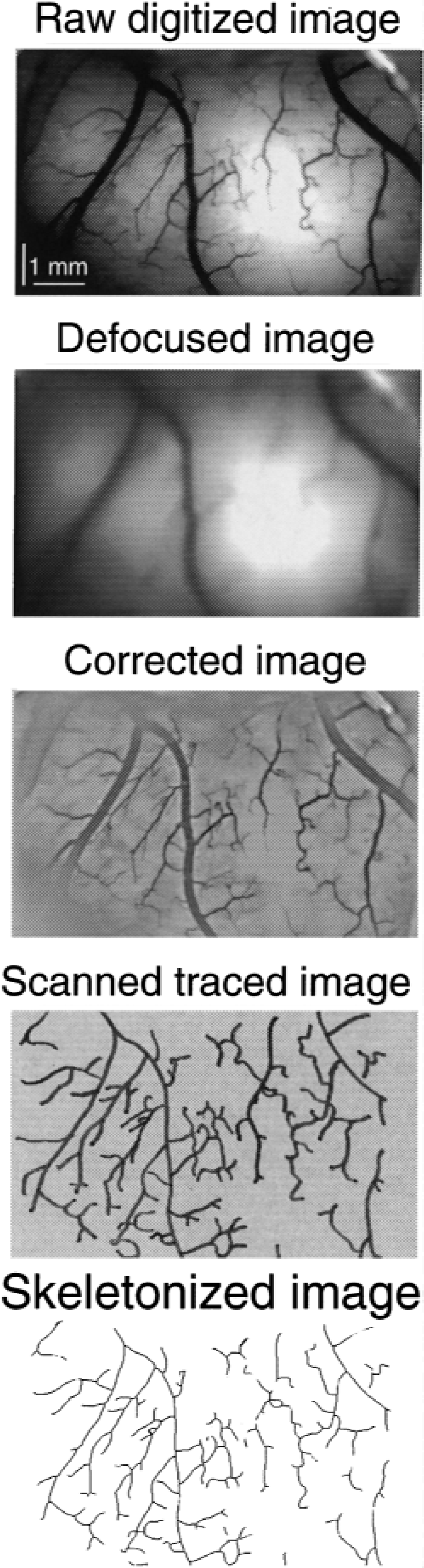
Processing the image of the cat brain cortex for a single pixel trace of the pial arterial network. The arterial network seen in Fig. 4 (first on the left) is used as an example for extracting the network's skeleton suitable for fractal analysis.

Assessing the curvature of the pial surface

Because the inner surface of the skull is not uniform because of the presence of imprints by vessels, gyri, and adhesions by the dura mater, the curvature of the pial surface was approximated by that of the outer surface of the skull where the burr hole location was known (Fig. 2, top panel). A cast of the skull of an adult cat was made in wax from the top to the level of the external auditory meati in horizontal position. The cast was securely mounted into a stereotaxic headholder (David Koppf Instruments, Tujunga, CA, U.S.A.) in horizontal position. A stainless steel spinal needle (18 gauge, Becton, Dickinson and Co., Rutherford, NJ, U.S.A.) was clamped into the electrode holder of the instrument in vertical position. Stereotaxic coordinates were acquired in a square raster of 31 × 17 mm reaching over the site of the burr hole (rostral medial corner at 6 mm, caudal medial corner at −25 mm from the bregma in the midline). Raster spacings were 1 mm along the X and Y, and 0.1 mm along the Z-coordinates. The needle probe at x, y raster coordinates was slowly lowered under visual control by a lupe until the tip made contact with the surface of the cast, at which point the Z-coordinate value, z, was read.

FIG. 2.

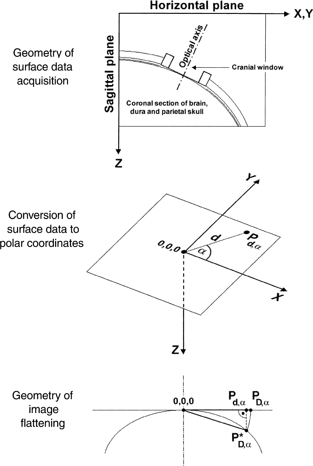
Schematic representation of geometrical correction of two-dimensional digitized images of pial networks for the three-dimensional curvature of the pial surface. Quantitative surface data was collected in the horizontal plane along the outer surface of the feline skull in a stereotaxic device (top). The surface data set was converted to polar coordinates with its origo (0,0,0) set to the center of the digitized image (middle). The orthograde (parallel to the optical axis) projection of the three-dimensional pial surface onto the digitized image was corrected by flattening based on the spatial data set (bottom). The curvature shown in the figure is exaggerated for demonstration purposes (notice the slight curvature profiles in Fig. 3.).

Each coronal and sagittal profile in the three-dimensional set of spatial coordinates (x, y, z) representing the surface geometry of the skull (Fig. 2, top panel) was fitted by a fourth order polynome, f(x) and f(y), respectively. The radius of the curved surface at each point, r, was determined from the parameters of the polynome as (1 + (f′(x))²)^1.5/ f′(x), and (1 + (f′(y))²)^1.5/ f′(y), where f′ and f′ denote the first and second derivatives, respectively. The distance from the outer surface of the skull to the pial surface was approximated by 3 mm, which was then subtracted from r yielding a corrected radius, r*. Curvatures in the sagittal and coronal planes, c_s and c_c, were calculated as 1/ r*.

Correcting for curvature by flattening

The steps of spatial transformations of image pixel data yielding an image corrected for the curvature of the pial network were as follows. Image dimensions were converted from pixel to millimeter to allow for geometric transformations in the spatial domain using the curvature data sets, c_s and c_c. c_s and c_c were geometrically transformed into c*_s and c*_c, which were centered rectangular to the optical axis of the video imaging system. In other words, X-, Y-, Z-coordinates of the image center became 0,0,0 mm (Fig. 2, middle panel). With this as reference point, polar coordinates were used in subsequent transformations. Three-dimensional image data of the networks were created by projecting each image point, P_d,α, in the focal plane in orthograde direction (parallel to the optical axis) onto the curved pial surface at the corresponding location P*_D,α. P*_D,α found in the three-dimensional image data set on the pial surface gave the coordinates of the corresponding location in the flattened image, P_D,α, in the two-dimensional focal plane. Finally, the network's image was visualized by using the non-uniformial interpolation function as implemented in the Grid Data Module of the MATLAB software (MathWorks, Natick, MA, U.S.A.).

Fractal analysis

The current fractal analysis of the pial vasculature is built on assessing the capacity dimension (D_cap) that derives from the self-similarity dimension, D (see Appendix). If D_cap is calculated by using contiguous, nonoverlapping boxes, the box counting dimension (D_BCM) is obtained (Liebovitch and Toth, 1989). In the authors' studies, the standard and extended version (Sandau and Kurz, 1996) of the box counting dimension were used.

Demonstrating additional fractal properties of the pial network: geometrical transformations

Fractal properties, such as self-similarity or self-affinity, scaling relationship, and scaling range (see Appendix) are characterized in a single parameter—the fractal dimension. Its value itself is no single proof of the fractal nature of the structure. Positive results of additional tests, such as when the network is found invariant to a variety of linear geometric transformations (for example, shift, rotation, scaling), should be used to firm up the indication as given by D that the pial network's design is most likely fractal. The transformations were performed (n = 1 to 30 times) in the following sequence: shifting the raw image horizontally by 10% of the image, rotating in increments of 3 n degrees, vertical scaling by a factor of 2.

Statistical analyses

The precision of linear regression fit used by box counting method (BCM), the coefficient of determination (r²), and the standard error of estimates were used as implemented in the SigmaStat program (SPSS; San Raffael, CA, U.S.A.).

The Mann–Whitney U test and the Student's t-test for independent samples tested the significance of difference between groups. Significance was accepted at a level P < 0.01. The mean squared error (MSE = SD² + bias²) was used to give a combined characterization of bias and variance in estimates of D_cap.

RESULTS

Transformation of pial networks from three-dimensional curved to two-dimensional planar geometry does not influence their fractal dimension in the imaged region of the brain cortex

The maximum curvature that was found for the pial surface within the imaged area of the brain cortex in the sagittal and coronal planes was 0.0216 mm⁻¹ and 0.0657 mm⁻¹, respectively. There was a gradual increase in the latero-frontal direction in the coronal profiles and a valley of minimal values in the sagittal profiles in the latero-caudal direction (Fig. 3A). As seen in Fig. 3B, these curvatures are so small that when they are used to remap the pixel values of a test pattern, the changes in the geometry, if any, are hardly noticeable. The same is seen for the exemplary arterial pial network No. 1. The insignificant influence of curvature on the planar fractal analysis of the pial networks also are demonstrated by the fact that D s for the raw and flattened (curvature corrected) networks differ only in the third decimal values (Table 1).

FIG. 3.

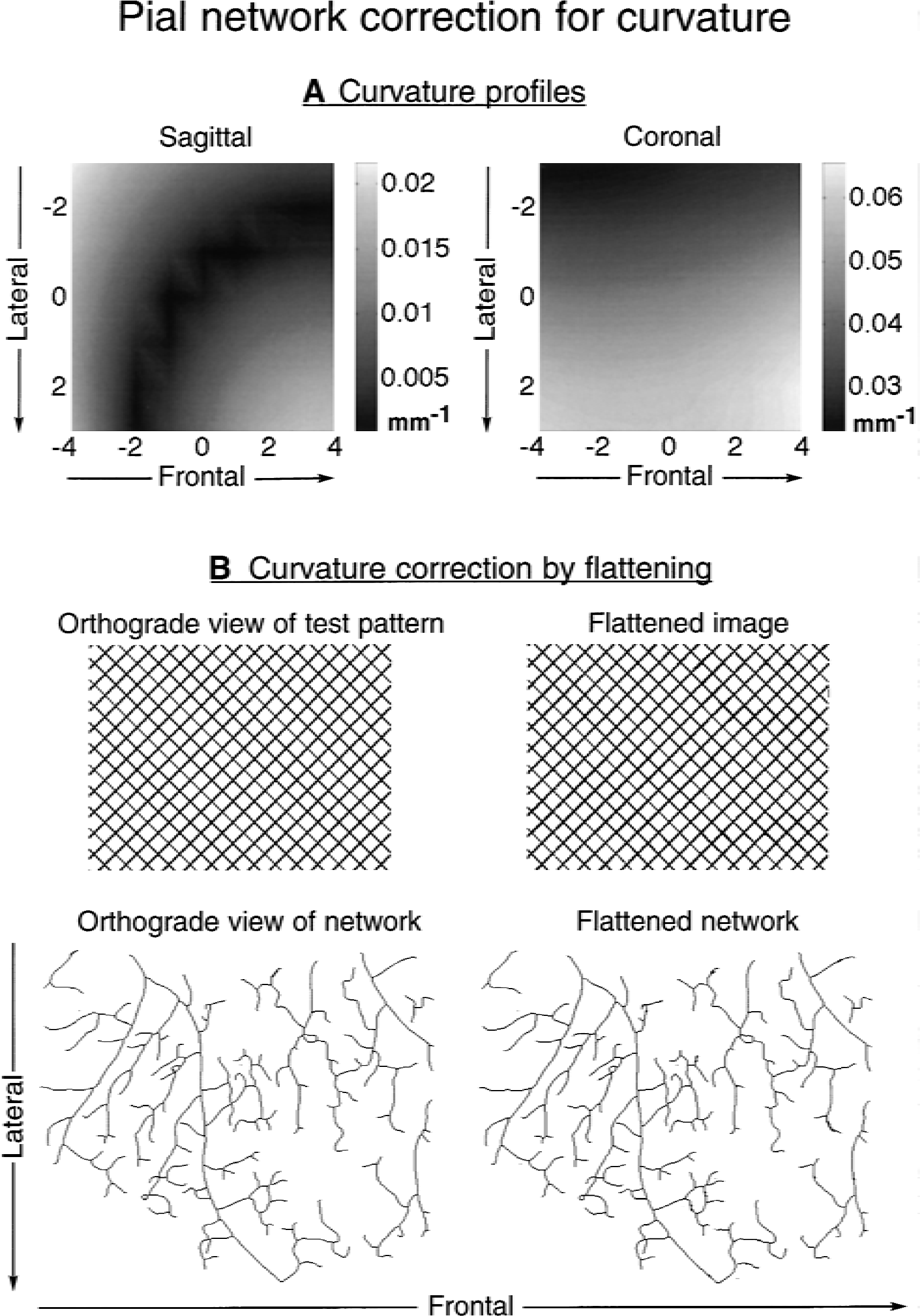
Impact of three-dimensional curvature of the pial surface on the planar representation of its vascular networks. The pial surface within the imaged area is only slightly curved in sagittal and coronal directions (A). This curvature thus does not alter the geometry of the projected images as tested on a test pattern and seen on a real arterial network No. 1 (B).

TABLE 1.

Estimated fractal capacity dimension for pial vessels

	Box counting method						Extended counting method
	Artery			Vein			Artery	Vein
n	D_cap ± SD	r² ± SD	SEE ± SD	D_cap ± SD	r² ± SD	SEE ± SD	D_cap ± SD	D_cap ± SD
Raw network
1	1.38 ± 0.01	0.98 ± 0.00	0.19 ± 0.01	1.35 ± 0.01	0.98 ± 0.00	0.19 ± 0.01	1.43 ± 0.00	1.40 ± 0.00
2	1.31 ± 0.01	0.98 ± 0.00	0.18 ± 0.01	1.32 ± 0.01	0.99 ± 0.00	0.17 ± 0.01	1.39 ± 0.00	1.39 ± 0.00
3	1.31 ± 0.01	0.98 ± 0.00	0.18 ± 0.01	1.28 ± 0.01	0.99 ± 0.00	0.16 ± 0.00	1.39 ± 0.00	1.36 ± 0.01
4	1.28 ± 0.01	0.98 ± 0.00	0.18 ± 0.01	1.30 ± 0.01	0.98 ± 0.00	0.19 ± 0.01	1.34 ± 0.00	1.35 ± 0.01
5	1.25 ± 0.01	0.98 ± 0.00	0.17 ± 0.01	1.29 ± 0.01	0.98 ± 0.00	0.19 ± 0.01	1.33 ± 0.01	1.36 ± 0.00
6	1.29 ± 0.01	0.98 ± 0.00	0.18 ± 0.01	1.30 ± 0.01	0.98 ± 0.00	0.18 ± 0.01	1.36 ± 0.00	1.37 ± 0.00
Mean ± SD	1.30 ± 0.04	0.98 ± 0.00	0.18 ± 0.01	1.31 ± 0.03	0.98 ± 0.00	0.18 ± 0.01	1.37 ± 0.04	1.37 ± 0.02
Flattened network
1	1.39 ± 0.01	0.98 ± 0.00	0.19 ± 0.01	1.36 ± 0.01	0.98 ± 0.00	0.19 ± 0.01	1.43 ± 0.01	1.40 ± 0.00
2	1.31 ± 0.01	0.99 ± 0.00	0.17 ± 0.01	1.31 ± 0.01	0.99 ± 0.00	0.16 ± 0.01	1.39 ± 0.00	1.39 ± 0.00
3	1.32 ± 0.01	0.98 ± 0.00	0.17 ± 0.01	1.28 ± 0.01	0.99 ± 0.00	0.16 ± 0.01	1.39 ± 0.00	1.36 ± 0.00
4	1.29 ± 0.01	0.98 ± 0.00	0.18 ± 0.01	1.31 ± 0.01	0.98 ± 0.00	0.18 ± 0.01	1.35 ± 0.00	1.35 ± 0.00
5	1.26 ± 0.01	0.99 ± 0.00	0.16 ± 0.01	1.31 ± 0.01	0.98 ± 0.00	0.18 ± 0.01	1.33 ± 0.01	1.36 ± 0.00
6	1.29 ± 0.01	0.99 ± 0.00	0.17 ± 0.01	1.31 ± 0.01	0.98 ± 0.00	0.17 ± 0.01	1.36 ± 0.00	1.37 ± 0.00
Mean ± SD	1.31 ± 0.04	0.98 ± 0.00	0.17 ± 0.01	1.31 ± 0.03	0.98 ± 0.00	0.17 ± 0.01	1.38 ± 0.03	1.37 ± 0.02
Student's t-test
P-value	0.65			0.47			0.89	0.87

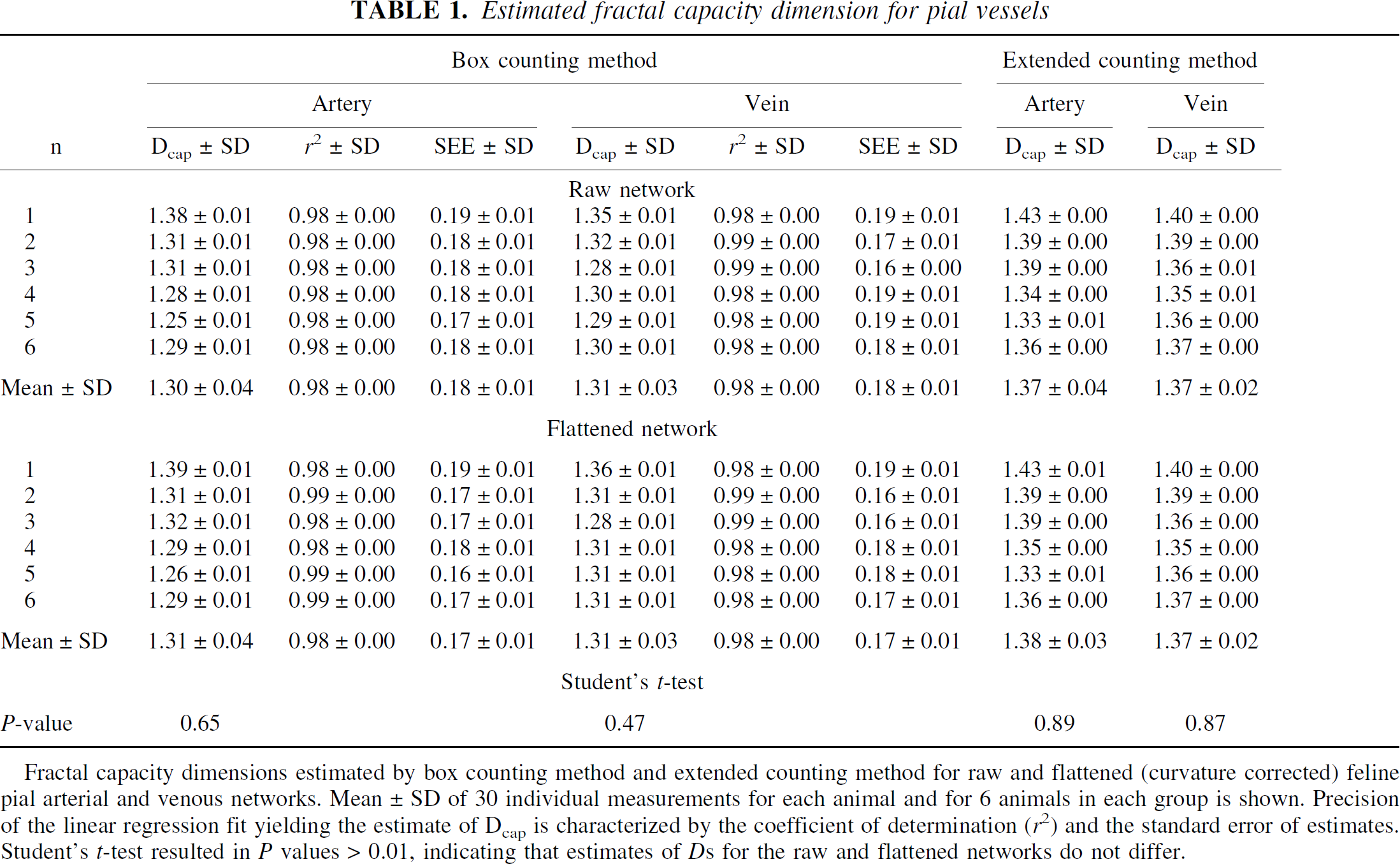
Fractal capacity dimensions estimated by box counting method and extended counting method for raw and flattened (curvature corrected) feline pial arterial and venous networks. Mean ± SD of 30 individual measurements for each animal and for 6 animals in each group is shown. Precision of the linear regression fit yielding the estimate of D_cap is characterized by the coefficient of determination (r²2) and the standard error of estimates. Student's t-test resulted in P values > 0.01, indicating that estimates of Ds for the raw and flattened networks do not differ.

Precision of the fractal methods used in the current study

It was found that the precision of the fractal methods (BCM, XCM) depends on type of the fractal structure being analyzed (Appendix). When BCM is applied to a branching structure (Mandelbrot tree) errors in its estimates of ${\overset{⁁}{D}}_{c a p}$ are much smaller than when it evaluates a nonbranching fractal (von Koch curve) as demonstrated in MSE values of 0.068 and 0.427, respectively. Extended counting method, however, proved better on nonbranching fractals than branching ones (MSE = 0.079 and 0.552, respectively).

Fractal dimensions of the pial vessel networks

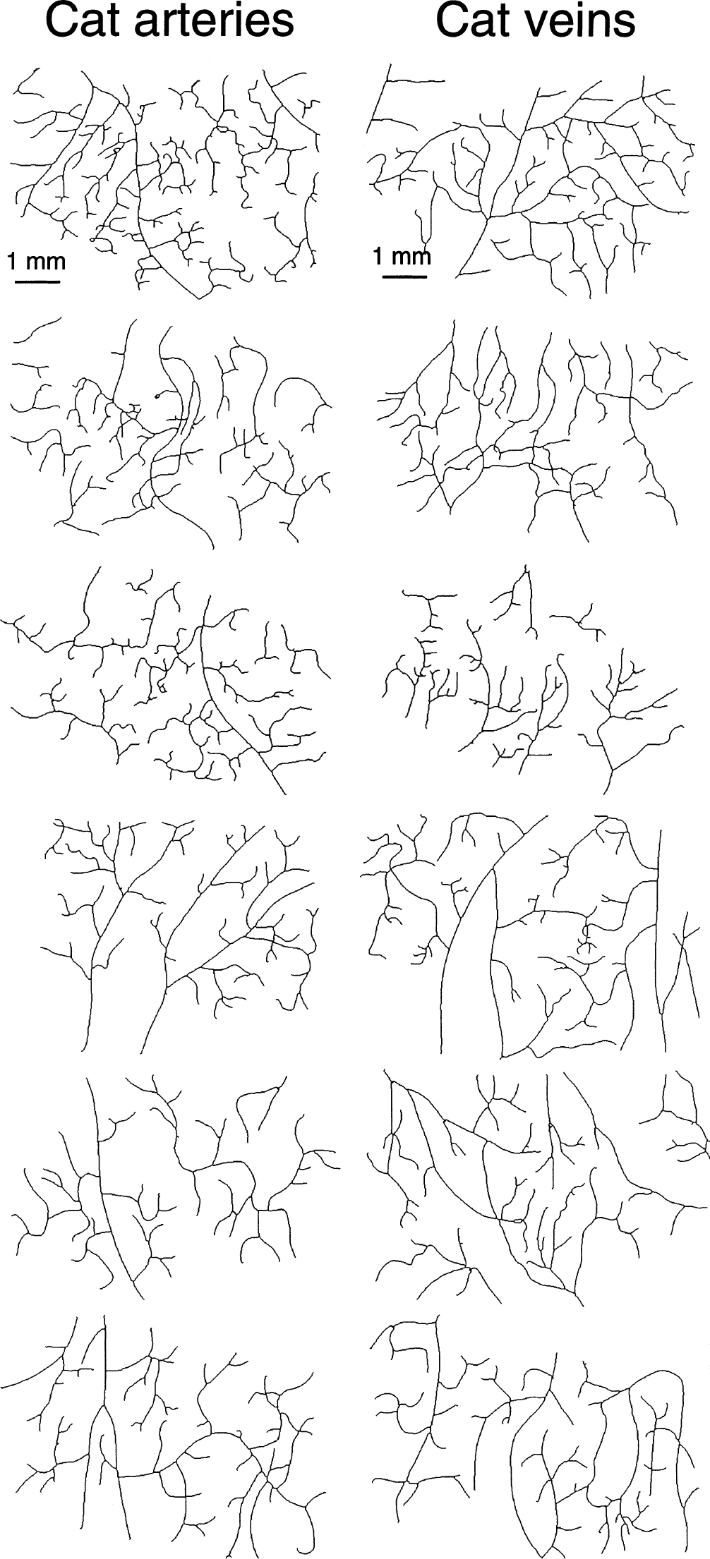
Networks analyzed (n = 6) are shown in Fig. 4. D_BCM and D_XCM found for these networks are shown in Table 1. As P > 0.01 values for the group means of the raw and curvature corrected networks demonstrate, D s determined by BCM and XCM were not significantly different. Box counting method or XCM found no difference between the fractal dimensions of the arterial and venous network groups in the cat using both Mann Whitney U test and Student's t-test. Respective D_BCM and D_XCM values also were similar for individual arterial and venous networks.

FIG. 4.

Single line tracings of feline arterial and venous pial networks obtained by digital image processing shown in Fig. 1. Fractal dimensions measured by the box and extended counting methods for these networks are shown in Table 1.

D_BCM and D_XCM values found for cat arteries, veins before and after linear geometric transformations (rotation, shifting, and scaling) were similar to those of a population of Mandelbrot trees within the ±1 SD range, indicating that these values reflect the fractal dimension of likely fractal structures (Fig. 5).

FIG. 5.

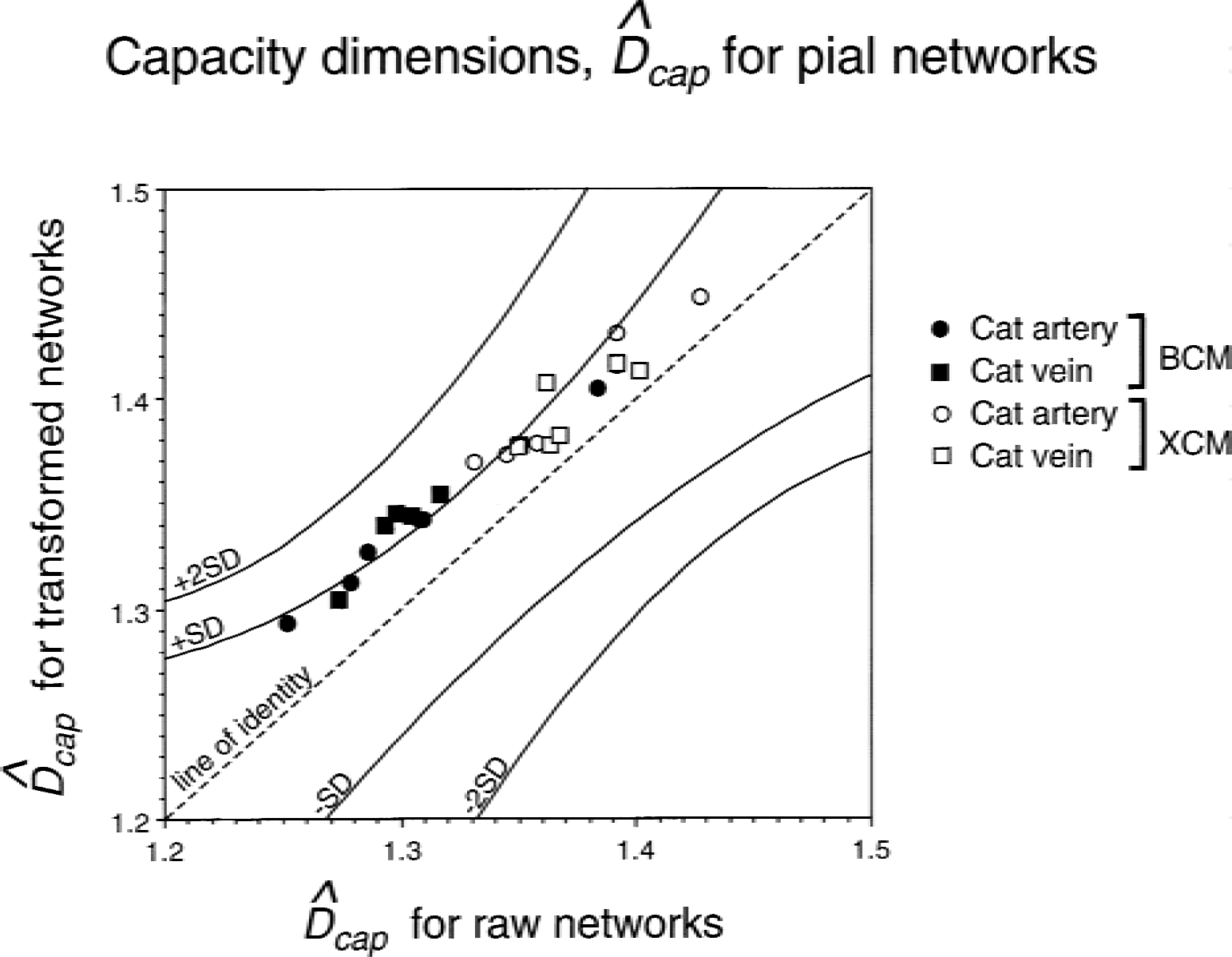
Demonstrating the fractal nature of pial networks in the cat by comparing the capacity dimensions obtained for raw and transformed networks. For the purpose of comparing raw and transformed ${\overset{⁁}{D}}_{c a p}$ S for real and ideal fractals, 44 ideal fractals of Mandelbrot tree type were generated with 1.2 < ${\overset{⁁}{D}}_{c a p}$ < 1.5 in steps of 0.1. ±1 SD and ±2 SD of ${\overset{⁁}{D}}_{c a p}$ S for these are shown. Fractal dimension is transformation invariant for true fractals. For most of the networks it falls within the ±1 SD range indicating that these networks are well approximated by the fractal model. Because of the insignificant influence of curvature on planar geometry, nonflattened digitized images of the networks were used for this figure.

DISCUSSION

Why is fractal analysis of pial networks useful?

The vascular system of the brain is special in that it has an equally complex extra-and intraparenchymal (that is, intracortical) system of supply and drainage. The extraparenchymal system can easily be visualized and was the subject of analysis in the current study. Repeated branching in the pial system produces length scales that can be captured in one picture. Fractal analysis is well suited to characterize scale invariant pattern present in the network. This feature is assessed by a single parameter—the fractal dimension, D. Fractal analysis is useful because it reduces characterization of a complex structure into finding its single descriptor. It is also relevant because it describes a fundamental property of the pial network—successive branching over the brain cortex starting with a few feeding and ultimately connecting to numerous perforating arteries.

The traditional classification approach also can lead to an evaluation of the fractal dimension of vessel networks based on taxonomical analysis of highly detailed data sets, such as the calculation of the Nelson dimension (Gan et al., 1993), or estimating the Tokunaga numbers (Turcotte et al., 1998). An obvious disadvantage of these methods is in the need for a detailed taxonomy, which requires large, high-definition networks to analyze. Such networks cannot be obtained on the pial surface in the cat. Therefore, the authors looked for alternatives in the analysis and found the calculation of the box dimension by BCM and its variant, XCM, simple yet effective.

Is computerized imaging of the pial vasculature adequate for fractal analysis?

Precision of fractal dimension depends on the details captured in the digitized image of the vessel network. The greater the definition the more accurate it becomes within the capabilities of the actual method used. Sensitivity of the video camera, quality of optics used, contrast of object influenced by light scattering, and geometrical resolution of the imager all determine what shows up on the images of the pial vasculature and what ultimately can be extracted as useful information for their fractal analysis. All of these components were selected carefully to minimize the loss of definition. Given the spatial resolution of the video imaging system, vessels of approximately 50 μm in diameter do not show up in the images because their image is projected onto only 1 or 2 pixels. Because of their small size, light scattering strongly affects them, thereby reducing their contrast in the raw image. When skeletonized, these pixels tend to turn white with a consequent loss of binary data in the network's tracing.

Alternatively, optical magnification could be increased and a higher definition image could be reconstructed from a set of smaller images taken at this higher magnification arranged in a square array. However, there are several limitations to this way of improving resolution. When imaging is performed in vivo, as in the current study, the absorption and scattering properties of blood perfusing the pial vessels and the microcirculation of the underlying parenchyma determine the optical contrast at which image features, such as vessels of minute dimension, can be extracted. As mentioned above, the authors' current setup limits the resolvable diameter to >50 μm, which is just more than the diameter of the perforating arterioles and venules, the last generation of the pial system. Therefore, the authors' images are almost complete; only the last segment is likely to be missing depending on hematocrit in the vessel and in the microcirculation of the parenchyma underneath. Because the fractal approach is aimed at finding correlation in a spatial, or for that matter temporal data set (Eke et al., 2000), if most of the features making the structure are captured in the data set and a fractal correlation is found, adding a minor fraction of missing information does not influence the outcome of the analysis. In other words, if the fractal design is present in the pial arterial and venous networks all the way to their second to last segment, capturing all the missing perforating segments would not make this design disappear.

In addition, arterial and venous networks are difficult to discern in the pial system. Because the current study was performed in vivo, the authors could simply find a solution to this problem by using bolus perfusion (Eke et al., 1979) to classify the vessels based on their transit dynamics—a method that could not be used if multiple imaging by mechanical scanning were to be chosen to improve on spatial resolution.

To make sure that the skeletonized images do contain the finest possible vascular details (that is, perforating arterioles and venules) detected by the video camera, manual tracing of the printed corrected image seemed necessary. This method seems subjective, but in fact, the human eye does an excellent job in pattern recognition with low-contrast grayscale images as compared with the performance of the NIH-Image program in this respect. An important precondition for reliable manual tracing of the networks is the digital image preprocessing eliminating the gradient from the background as shown in Fig. 1. In these images (Fig. 1, middle), the segments of the networks are easy to identify; therefore, the manual tracing method under these specific circumstances should be regarded as reliable.

The video images captured all but one generation of the pial networks. The question may arise: Is the scaling range present in these images adequate for a fractal analysis? The length scales were approximately one magnitude, which is not sufficient for a fractal analysis if the analysis is based on evaluating self-similarity on the length scale. The current fractal analysis using BCM and XCM, however, were statistical methods based on evaluating the self-similarity of the probability density functions at different spatial scales (Bassingthwaighte et al., 1994). These scales, as determined by the counting box dimensions, were approximately two magnitudes, which is adequate for a statistical spatial and temporal (Eke et al., 2000) fractal analysis.

Two-dimensional capturing of the slightly curved pial network (three-dimensional) does not distort its fractal structure

As shown in Table 1, correction for the three-dimensional curvature of the pial surface by flattening of the acquired images do not have any significant influence on the fractal dimensions as determined by BCM and XCM because the deviation of the pial networks from two-dimensional is very slight (Fig. 3). Estimating the curvature by collecting surface data on the outer surface of the skull seems justified, because local disturbances in the surface data—had they been collected from the internal surface of the skull—due to imprints would have resulted in a noisy data set inadequate for image flattening. The current raw spatial data was not smoothed before fitting by the fourth order polynome, still the resulting curvature maps turned out to be free of erratic gradients (Fig. 3A). The method of flattening (Fig. 2) has some limitations. The linear approximation used in finding P*_D,α can only be used for slightly curved convex surfaces, like the pial surface in the current study. It is not suitable for more curved and concave surfaces, like the retinal networks. Nevertheless, the authors' treatment of curvature can provide a guide for the application of fractal analysis in other vascular networks laid out on curved surfaces. In addition, flattening cannot be applied to uneven surfaces where there is local swapping between being convex and concave. In the current studies, these limitations did not interfere with the outcome of the results, therefore Fig. 5 was created based on D s evaluated for uncorrected nonflattened network (Table 1).

Notably, BCM and XCM can be configured to evaluate one-dimensional, two-dimensional, and three-dimensional structures depending on how the algorithm is implemented (see Fractal dimensions in Appendix). In the current studies, the algorithm of these methods was implemented for two-dimensional, planar structures. Using BCM and XCM on nonflattened images is not a violation of their applicability, because these images do contain two-dimensional spatial data of slightly curved three-dimensional vascular networks.

Numerical testing of fractal methods for their precision estimating the fractal dimension of pial networks

The usual approach to testing the precision of fractal methods is to apply them to ideal fractal objects of known D and compare their true and estimated D s. The authors found that the overall character of the fractal objects used in testing also mattered. Mean squared error as the measure of precision of the estimates depended not only on the method, BCM or XCM, but on the type of object to which it was applied. Box counting method was better on treelike fractals, whereas XCM was better on nonbranching fractals. This circumstance was not recognized earlier (Sandau and Kurz, 1996), although undoubtedly it is important for future studies of fractal properties of vascular networks. This observation led the authors to realize the importance of finding the best possible test object realistically modeling the pial network. Using the L-system (Lindenmayer, 1968), one such fractal tree was generated (Appendix, Fig. 6C) but could not be used for testing because of its unknown true D. An a priori knowledge of true D is the prerequisite of the use of an ideal fractal for numerical testing. This issue is further complicated by the fact that knowledge of true D in and of itself is insufficient for testing. True D should be variable within a wide range into which D of planar vascular networks may fall. Further studies in this direction are needed to make testing of fractal methods for real vascular networks conclusive.

FIG. 6.

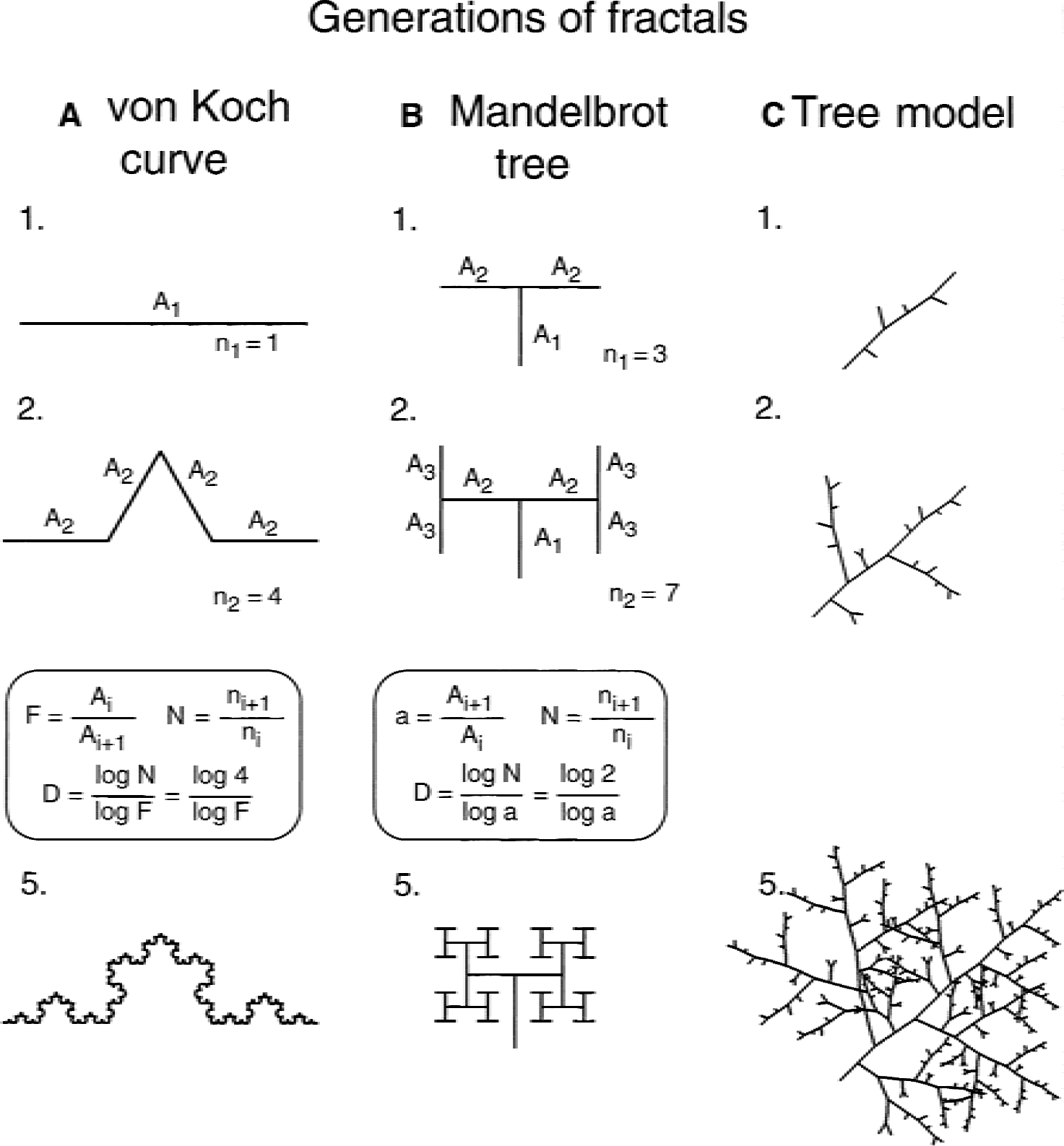
Evolution of fractal structures. Nonbranching von Koch curve (A), branching Mandelbrot tree (B), and a branching tree (C) closely resembling the pial networks shown in Fig. 4. Structures A and B are similar in that they are produced by single sets of generation rules. Structure C was generated using the L-system by combining two generation rules.

Which fractal method is better: which D to trust?

Box counting method has traditionally been among the first choice of methods for spatial fractal analysis, although it has three potential problems. The first problem relates to the fact that D_BCM is calculated as the slope of a linear regression plot N (L). The slope depends on the box size used (Appendix, Fig. 7) and the range of data fitted (Pancio and Sterling, 1995), in addition to the number of data pairs used. To increase the number of data pairs in the analysis, the box size was not changed after the common practice as power of 2 (2, 4, 8, etc.), but rather in steps of 1 (1, 2, 3, etc.). In addition, if N s did not differ for two or more contiguous L s, only one N from each group was used. The second problem is associated with a prerequisite of D having to be motion invariant, which means D has to be independent of the starting location and the orientation of the object relative to the grid. D_BCM, however, is not motion invariant. The third problem relates to maximum property by which if two objects with different fractal dimensions are overlaid, the resulting dimension will be determined by the one with the higher dimension (Peitgen et al., 1992). Extended counting method was developed when these problems became evident resulting in an efficient method for which these problems are either eliminated (linear regression), or reduced (motion invariance), or appear to be less pronounced (maximum property) (Sandau and Kurz, 1996).

FIG. 7.

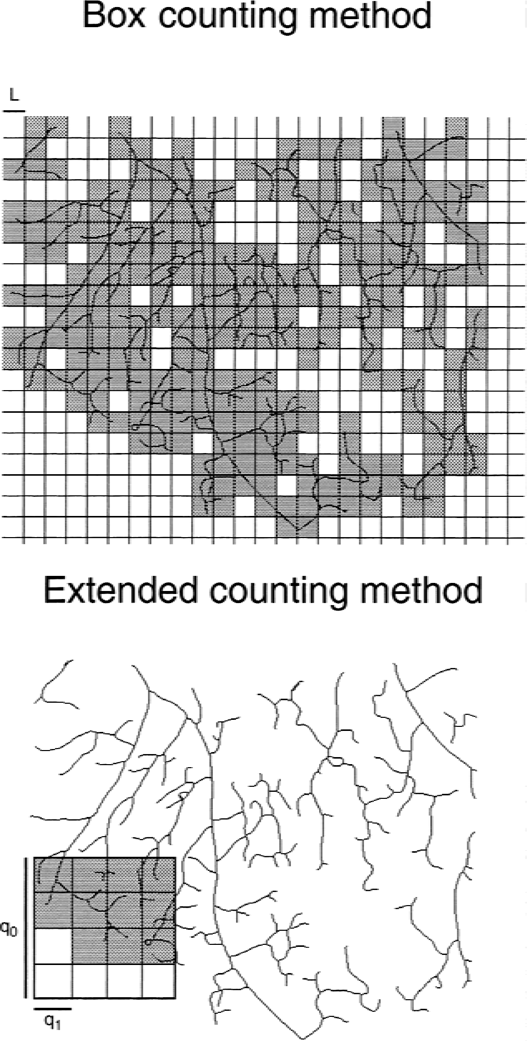
Concept of the box and extended counting methods. Box counting method (top) applied to a pial network is demonstrated: a grid of boxes of the size of the network is overlaid onto its skeletonized image. Boxes covering any piece of the vasculature (shown in gray) are counted at different box sizes. With the extended counting method (bottom) a grid of boxes smaller than the size of the network is used. It is moved along the object in freely chosen steps smaller than q_o, whereas small boxes containing any piece of the object is being counted (shown in gray).

The authors found, however, that XCM cannot replace BCM in fractal analysis, because the precision of these methods depends on the nature of the object they evaluate (Appendix, Fig. 8). The similarity of ${\overset{⁁}{D}}_{c a p} s$ that was found for the pial networks by BCM and XCM (Table 1) suggests that the performance of these two methods on real networks, in contrast with what was found on Mandelbrot trees (Appendix, Fig. 8), may be similar; however, the claim cannot be proven at the moment having no way of generating realistic vascular models with known and variable D s for testing. For the same reason, not knowing the bias and variance in ${\overset{⁁}{D}}_{c a p} s$ , it cannot be proven that these estimates are correct in terms of the true D of the networks. However, similarity of ${\overset{⁁}{D}}_{c a p} s$ found for the raw and transformed networks (Fig. 5) indicates that the pial networks are close to ideal fractals structures. If so, ${\overset{⁁}{D}}_{c a p} s$ are meaningful measures of the networks' space filling properties, and ${\overset{⁁}{D}}_{c a p} s$ found for different animals of the same species can be compared. A comparison of ${\overset{⁁}{D}}_{c a p} s$ obtained for different species, or for that matter networks of the same species at different stages of development, would only be possible if BCM and XCM were tested on realistic model networks specific to the actual networks being compared. The result of such tests should prove that BCM and XCM provides estimates for D with comparable bias and variance in these cases.

FIG. 8.

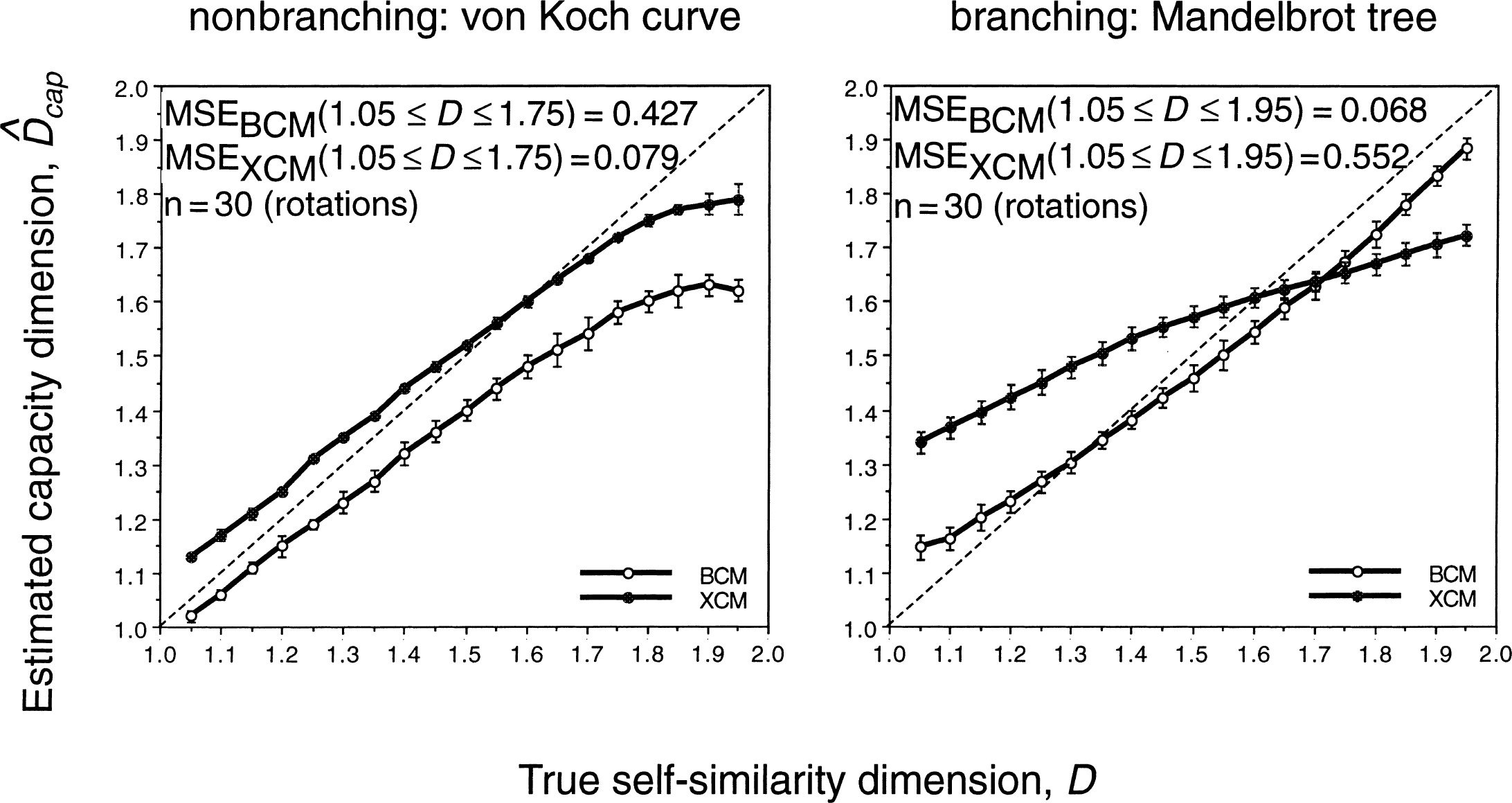
Estimated fractal dimensions for exact nonbranching and branching geometric fractal structures. Exact single fractal structures shown in Fig. 6 were used to test the precision of the box counting (BCM) and extended counting (XCM) methods in estimating the capacity dimension (D_cap) of the structure. Dotted lines indicate the line of identity at which estimate of D equals true D. Deviation from this line is the bias in the estimate, whereas bars of SD indicate the variance. The mean squared error (MSE = SD² + bias²) was used to give a combined characterization of bias and variance in estimates of D_cap. Each point represents the mean of 30 estimates of the same structure rotated by 3 degrees.

Interpretation of the fractal estimates determined for the pial vascular networks

Detailed studies of the vascular architecture in the rat brain cortex by Bär (1980) reported the presence of a modular system of arterial supply. The vascular system Bär described appears to be fractal, which he could not possibly have recognized at the time. The current findings identify a fractal arborization scheme in the pial system, which extends the observations of Bär from the intra-to the extraparenchymal segments of the vascular system of the brain. This is most likely not a coincidence, because fractals render themselves as a genuine model of producing modular networks from self-similar elements with each generation supplying a progressively smaller tissue volume. Recent findings indicate that fractal structures indeed are ideally suited to develop optimized networks of flow distribution by minimizing the viscous dissipation of energy in such systems (West et al., 1997, 1999). Further evidence to the fractal organization in vascular systems are the consistency in changes of vessel diameter, segment length, and wall thickness across many generations reported for the mesenteric and renal arterial trees long before the fractal era in medical sciences began (Suwa et al., 1963, Suwa and Takahashi, 1971).

In analyzing the extraparenchymal part of the vascular trees no difference between the fractal dimension of the arterial and venous trees in the cat was found. The current findings identify identical design concepts in these systems of blood supply and drainage over the brain cortex, which corresponds well with the similarity of the intraparenchymal anatomy of the arterial and venous vascular trees reported by Duvernoy for the human brain (Duvernoy et al., 1981). Similar observations were reported for other vessel systems, such as the one by Landini for the retina (Landini et al., 1993).

Conclusion

The fractal analysis is a model-based approach (Bassingthwaighte, 1991). By demonstrating the similarity of ${\overset{⁁}{D}}_{c a p} s$ for the raw and geometrically transformed pial networks, the authors found basis to regard the fractal model as correct to describe the scale invariant bifurcation patterns in these networks. Specific models are still lacking. These models would be needed to firm up the estimates of the methods, and to yield ${\overset{⁁}{D}}_{c a p} s$ suitable to be used in simulation studies to generate artificial networks with fractal dimension of real ones.

The authors' approach developed for a two-dimensional analysis can be adapted to three dimensions, and then can be applied to the analysis of the intracortical arterial and venous trees. This step will be feasible to undertake once a method for a three-dimensional reconstruction of the intracortical vascular trees becomes available. Combined use of the two-and three-dimensional fractal analyses seem necessary to describe the change in spatial complexity in cerebro-cortical blood supply in the course of phylogeny or aging. It seems worthwhile to repeat the studies evaluating structural changes in the pial vasculature (Hudetz et al., 1987; Jiang et al., 1994; Mchedlishvili and Kuridze, 1984; Singhal et al., 1973) and to compare and correlate the fractal and taxonomical descriptors for these networks found in different experimental conditions.

Fractals do not have exact definition, only properties (Falconer, 1990). The authors obtained one, the capacity dimension, in the current study. Others could be evaluated in the future, such as self-similarity in vessel diameter or length ratios, etc. There are reports indicating that these properties are self-similar in other vascular beds (Gan et al., 1993; Jiang et al., 1994; West et al., 1997) and that the fractal model is optimal to produce transport systems, among them that of the vessel networks (West et al., 1999).

Footnotes

Acknowledgments:

The authors thank Drs. James B. Bassingthwaighte and Tibor Toth for stimulating discussions and critical evaluation of an earlier version of the manuscript.

APPENDIX

References

Bär

(1980) The vascular system of the cerbral cortex. Adv Anat Embriol Cell Biol 59:1–63

Bassingthwaighte

van Beek

JHGM

King

(1990) Fractal branchings: The basis of myocardial flow heterogeneities? Ann NY Acad Sci 591:392–401

Bassingthwaighte

(1991) Chaos in the fractal arteriolar network. In: The resistance vasculature ( Bevan

Halpern

ed), Totowa: Humana Press, pp 431–449

Bassingthwaighte

Liebovitch

West

(1994) Fractal physiology. Molvany, Oxford: Oxford University Press, pp 11–44

Duvernoy

Delon

Vannson

(1981) Cortical blood vessels of the human brain. Brain Res Bull 7:519–579

Eke

Hutiray

Kovach

AGB

(1979) Induced hemodilution detected by reflectometry for measuring microregional blood flow and blood volume in cat brain cortex. Am J Physiol 236:H759–H768

Eke

(1983) Integrated microvessel diameter and microregional blood content as determined by cerebrocortical video reflectometry. In: The cerebral veins ( Auer

Loew

, eds), Wien: Springer-Verlag, pp 249–252

Eke

Hermán

Bassingthwaighte

Raymond

Percival

Cannon

Balla

Ikrényi

(2000) Physiological time series: Distinguishing fractal noises from motions. Pflügers Arch 439:403–415

Falconer

(1990) Fractal geometry. Chichester, U.K.: Wiley and Sons

10.

Family

Masters

Platt

(1989) Fractal pattern formation in human retinal vessels. Physica D 38:98–103

11.

Gan

Tian

Yen

Kassab

(1993) Morphometry of the dog pulmonary venous tree. J Appl Physiol 75:432–440

12.

Gazit

Baish

Safabakhsh

Leunig

Baxter

Jain

(1997) Fractal characteristics of tumor vascular architecture during tumor growth and regression. Microcirculation 4:395–402

13.

Glenny

Robertson

Yamashiro

Bassingthwaighte

(1991) Applications of fractal analysis to physiology. J Appl Physiol 70:2351–2367

14.

Grassberger

Procaccia

(1983) Measuring the strangeness of strange attractors. Physica D 9:189–208

15.

Hudetz

Conger

Halsey

Pal

Dohan

Kovach

(1987) Pressure distribution in the pial arterial system of rats based on morphometric data and mathematical models. J Cereb Blood Flow Metab 7:342–355

16.

Jiang

Kassab

Fung

(1994) Diameter-defined Strahler system and connectivity matrix of the pulmonary arterial tree. J Appl Physiol 76:882–892

17.

Kurz

Wilting

Sandau

Christ

(1998) Automated evaluation of angiogenic effects mediated by VEGF and P1GF homo- and heterodimers. Microvasc Res 55:92–102

18.

Landini

Misson

Murray

(1993) Fractal analysis of the normal human retinal fluorescein angiogram. Curr Eye Res 12:23–27

19.

Liebovitch

Toth

(1989) A fast algorithm to determine fractal dimensions by box counting. Phys Lett 141(8,9):386–340

20.

Lindenmayer

(1968) Mathematical models for cellular interaction in development. Parts I and II. J Theor Biol 18:280–315

21.

Mandelbrot

(1983) The fractal geometry of nature. San Francisco, CA: W.H. Freeman and Co

22.

McHedlishvili

Kuridze

(1984) The modular organization of the pial arterial system in phylogeny. J Cereb Blood Flow Metab 4:391–396

23.

Pancio

Sterling

(1995) Retinal neurons and vessels are not fractal but space-filling. J Comparative Neurol 361:470–490

24.

Peitgen

H-O

Jürgens

Saupe

(1992) Chaos and fractals. New York: Springer-Verlag

25.

Sandau

Kurz

(1996) Measuring fractal dimension and complexity – an alternative approach with an application. J Microsc 186: 164–176

26.

Singhal

Henderson

Horsfield

Harding

Cumming

(1973) Morphology of the pulmonary arterial tree. Circ Res 33:190–200

27.

Strahler

(1957) Quantitative analysis of watershed geomorphology. Trans Am Geophys Union 38:913–920

28.

Suwa

Niwa

Fukasawa

Sasaki

(1963) Estimation of intravascular blood pressure gradient by mathematical analysis of arterial casts. Tohoku J Exp Med 79:168–198

29.

Suwa

Takahashi

(1971) Morphological and morphometrical analysis of circulation in hypertension and ischemic kidney. Munich: Urban & Schwarzenberg

30.

Turcotte

Pelletier

Newman

(1998) Networks with side branching in biology. J Theor Biol 193:577–592

31.

Van Beek

JHGM

Bassingthwaighte

Roger

(1989) Regional myocardial flow heterogeneity explained with fractal networks. Fractal Vascular Networks 249–257

32.

Weibel

(1991) Fractal geometry: A design principle for living organisms. Am J Physiol 261:L361–369

33.

West

Brown

Enquist

(1997) A general model for the origin of allometric scaling laws in biology. Science 276:122–126

34.

West

Brown

Enquist

(1999) The fourth dimension of life: Fractal geometry and allometric scaling of organisms. Science 284:1677–1679

35.

Holmes

Moore

Chen

Arkin

(1994) Microvascular architecture within the pig kidney cortex. Microvasc Res 47:293–307

Fractal Branching Pattern in the Pial Vasculature in the Cat

Abstract

Keywords

MATERIALS AND METHODS

Video imaging of the pial vasculature

Digital image processing

Assessing the curvature of the pial surface

Correcting for curvature by flattening

Fractal analysis

Demonstrating additional fractal properties of the pial network: geometrical transformations

Statistical analyses

RESULTS

Transformation of pial networks from three-dimensional curved to two-dimensional planar geometry does not influence their fractal dimension in the imaged region of the brain cortex

Precision of the fractal methods used in the current study

Fractal dimensions of the pial vessel networks

DISCUSSION

Why is fractal analysis of pial networks useful?

Is computerized imaging of the pial vasculature adequate for fractal analysis?

Two-dimensional capturing of the slightly curved pial network (three-dimensional) does not distort its fractal structure

Numerical testing of fractal methods for their precision estimating the fractal dimension of pial networks

Which fractal method is better: which D to trust?

Interpretation of the fractal estimates determined for the pial vascular networks

Conclusion

Footnotes

Acknowledgments:

APPENDIX

References