Systems Analysis of Functional Magnetic Resonance Imaging Data Using a Physiologic Model of Venous Oxygenation

Abstract

The authors revisit a simple mathematical model, presented in previous work, that characterizes the response of cerebral venous oxygenation to changes in blood flow and oxygen consumption. This physiologically based model can qualitatively duplicate the results of several recent empirical studies in which other authors have tested the hypothesis of linearity in the functional magnetic resonance imaging (fMRI) response to task activation, in that the experimentally found nearly linear behavior of the system and also its subtle departures from linearity are both predicted by simulations of the model. The model is simple enough that its equations can be explicitly solved. Moreover, an amended model that incorporates a varying cerebral blood volume parameter is found to have similar if not better consistency with the empirical data; indeed, this “extended” model is shown to be solvable by the same differential equation as the authors' simple one, wherein the volume is fixed as a constant. These investigations lend further indirect support to the blood oxygen level-dependent hypothesis of venous deoxyhemoglobin as the primary mechanism for fMRI signal changes during task activation, as well as for the authors' simple system as a useful physiologic model thereof. Although the authors' mathematical model does not formally represent a linear system with respect to the flow input, its underlying linear character may help partially explain the “nearly” linear behavior of the fMRI response.

Since its inception some years ago, the field of functional magnetic resonance imaging (fMRI) has been an area of active research. As the field has matured, several groups are now using fMRI to study various aspects of cerebral physiology with functional activation (Buxton and Frank, 1997; Duyn et al., 1994; Ernst and Hennig, 1994; Glover, 1999; Hathout et al., 1999; Hu et al., 1997; Kennan et al., 1997; Menon et al., 1995; Ogawa et al., 1993). Active research areas include a reexamination of the notion of an initial uncoupling of flow from metabolism with cortical activation (Buxton and Frank, 1997), and the cerebral physiology underlying the “early response” phenomenon (Ernst and Hennig, 1994; Hu et al., 1997; Menon et al., 1995).

As fMRI research begins to delve into the cerebral physiology underlying brain activation, many investigators are modeling the fMRI response to task activation within the framework of an input/output system. In this context, the input function models the timing of task activation and the output function the resulting fMRI signal. In the recent seminal work of Boynton et al. (1996), the cerebral response is modeled as a linear time-invariant (LTI) system, under the hypothesis that fMRI responses are proportional to local neural activity averaged over time. Their empirical data measuring the fMRI response to visual stimuli are roughly consistent with these assumptions. If correct, such a model enables the powerful machinery of linear systems analysis to be brought fully to bear, allowing the computation of an impulse response function that completely characterizes the system in that the output function to any given input could be predicted by convolution (Boynton et al., 1996; Dale and Buckner, 1997). It would also allow the deconvolution of the response to any single stimulus in a mixed-stimulus pattern (Dale and Buckner, 1997).

Boynton et al. (1996) tested the LTI hypothesis in several experiments. In the most important, the fMRI response to a visual task is first measured for stimulus pulses of varying duration. Then, the responses to pulses of longer duration are compared with the net signal reconstructed by summing time-shifted copies of shorter pulses. For example, according to the LTI model, the response to a 12-second stimulus pulse should be calculable by summing 4 copies of the 3-second stimulus response, shifted in time by 0, 3, 6, and 9 seconds, respectively. Boynton et al. found that although the data are generally consistent with the LTI model, there is a subtle yet systematic failure of the predictions: the summed responses to shorter pulses tend to overestimate the response to the longer pulse during the activation phase, and they underestimate the response during the postactivation phase. The reasons for these phenomena are unclear, but the authors attribute these discrepancies to possible neural adaptation with the longer pulses (Boynton et al., 1996).

Similarly, the recent intriguing work by Dale and Buckner (1997) tested the hypotheses of the LTI model by subtracting the fMRI response to a single trial, again using a visual stimulus, from the measured signal response to two identical trials presented in rapid succession. If the model is linear, then the net difference signal should, in effect, isolate the response to the second trial; moreover, if the model is time-invariant, then this calculated second trial response should coincide with an appropriately time-shifted signal response to the single trial. Here again, the authors found results that are generally consistent with an LTI system but that likewise display a subtle systematic departure from ideal LTI behavior in that the calculated difference signal contains a slight undershoot in the declining phase when compared with the time-shifted single trial response.

The current article examines these phenomena of “near-linearity” within the framework of a simple input/output system that the authors have presented previously (Hathout et al., 1995, 1999). Although somewhat primitive in its assumptions, the model is appealing because its underlying equations are derived from physiologic rather than parametric modeling. Indeed, despite its simplicity, it succeeds in predicting the results found empirically by the above authors in their respective works more completely than parametric LTI modeling. Further, a more generalized model presented later in this paper, incorporating assumptions used by Buxton et al. (1998) in their investigations, succeeds even better in matching the empirical results, predicting even subtler aspects of the departures from linearity.

Any conclusions to be drawn from such mathematical modeling are necessarily weak, in that nothing can be definitively proven by mere consistency with computer simulations; however, the success of the model in its predictions may shed light on some basic questions underlying the system, such as the mechanism of the blood oxygen level-dependent (BOLD) effect and the mechanical properties of the venous compartment, as well as providing a partial explanation for both the near-linearity of the fMRI signal response and its subtle departures from ideal LTI behavior.

MATERIALS AND METHODS

Mathematical models

Simple model.

Essentially, the authors' model computes the change in venous oxyhemoglobin concentration ([O₂]_v) based on changes in regional cerebral blood flow (F), cerebral blood volume (V), and oxygen consumption (C′). In previous publications, a full derivation of the model is described and simulated results are correlated with existing fMRI data (Hathout et al., 1995, 1999). As an input/output system, the model has three input functions (F, V, and C′) and one output ([O₂]_v). The authors chose to study the output function of venous oxyhemoglobin because the BOLD hypothesis postulates that fMRI signal changes occur as a result of variations in venous deoxyhemoglobin concentration. Oxyhemoglobin was chosen rather than deoxyhemoglobin to parallel the changes in fMRI signal (that is, it increases with task activation), but the two are entirely mathematically equivalent. A simplified derivation of the model and its equations is presented here.

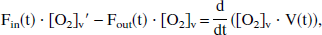
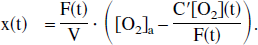
To start, a mass-balance approach is used to calculate the oxygen concentration in the local capillary bed being emptied into the venous pool. This end-capillary O₂ concentration, termed [O₂]′_v(t), therefore varies with task activation and the resulting changes in blood flow and oxygen consumption. To derive this relationship, Fick's law is used, whereby regional oxygen consumption (C′[O₂]) can be written as the product of cerebral blood flow (F) and the difference between arterial oxygen concentration ([O₂]_a) and end-capillary oxygen concentration ([O₂]′_v):

${\mathrm{C}}^{\prime }[{\mathrm{O}}_2]=\mathrm{F}\cdot ({[{\mathrm{O}}_2]}_{\mathrm{a}}-{[{\mathrm{O}}_2{]}^{\prime }}_{\hspace{0.17em}\hspace{0.17em}\hspace{0.17em}\hspace{0.17em}\mathrm{v}}).$

(1)

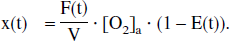
In terms of the oxygen extraction fraction E(t) = 1 − [O₂]′_v/[O₂]_a, the following can be written:

${\mathrm{C}}^{\prime }[{\mathrm{O}}_2]=\mathrm{F}(\mathrm{t})\cdot {[{\mathrm{O}}_2]}_{\mathrm{a}}\cdot \mathrm{E}(\mathrm{t}),$

(2)

where if consumption remains constant, then E(t) · F(t) remains constant.

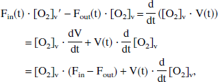
To yield a true venous oxyhemoglobin level at time t, [O₂]_v(t), the incremental [O₂]′_v(t) is assumed to be flowing into a well-mixed venous pool, where the existing venous oxygen concentration is [O₂]_v. Therefore, the mass-balance equation for venous oxygen concentration can be written as

$\mathrm{F}(\mathrm{t})\cdot {[{\mathrm{O}}_2{]}^{\prime }}_{\hspace{0.17em}\hspace{0.17em}\hspace{0.17em}\mathrm{v}}(\mathrm{t})-\mathrm{F}(\mathrm{t})\cdot {[{\mathrm{O}}_2]}_{\mathrm{v}}(\mathrm{t})=\frac{\mathrm{d}}{\text{dt}}({[{\mathrm{O}}_2]}_{\mathrm{v}}(\mathrm{t})\cdot \mathrm{V})$

(3)

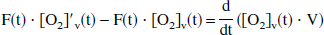
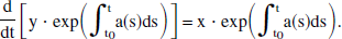
where the right side of the equation represents the time derivative of total venous oxygen content and the left side represents the difference between inflowing and outflowing oxygen flux. The solution of the general form of this equation has been presented elsewhere (Hathout et al., 1995), where the cerebral blood volume V is considered a time variable, and where an exponential form of E(t) is assumed. In the even simpler model of current interest, V is assumed to be constant, so that the following may be written:

$\mathrm{F}(\mathrm{t})\cdot {[{\mathrm{O}}_2{]}^{\prime }}_{\hspace{0.17em}\hspace{0.17em}\mathrm{v}}(\mathrm{t})-\mathrm{F}(\mathrm{t})\cdot {[{\mathrm{O}}_2]}_{\mathrm{v}}(\mathrm{t})=\mathrm{V}\cdot \frac{\mathrm{d}}{\text{dt}}({[{\mathrm{O}}_2]}_{\mathrm{v}}(\mathrm{t})).$

(4)

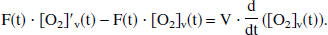
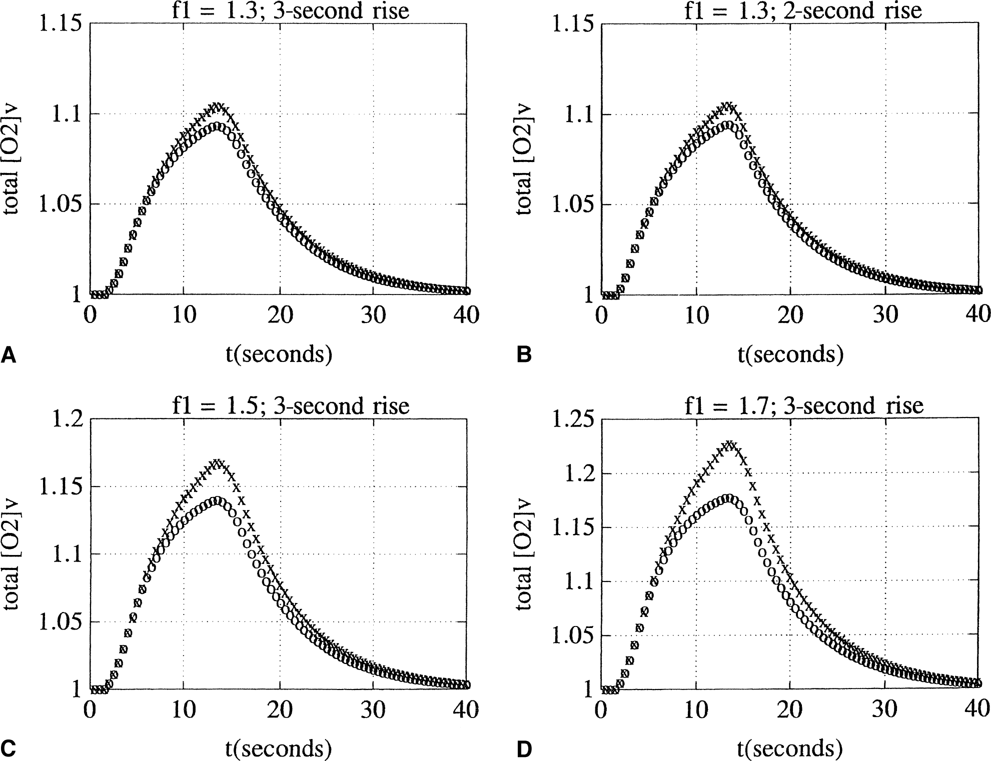
Equation 4 describes the dynamic change of [O₂]_v(t) to a new equilibrium value after a change in blood flow F, and hence models the lag inherent in the response of cerebral venous oxygenation to changes in cerebral blood flow. This equation can now be solved explicitly. For ease of legibility, the following new variables are introduced:

$\begin{array}{lll}\mathrm{y}(\mathrm{t})\hfill & =\hfill & {[{\mathrm{O}}_2]}_{\mathrm{v}}(\mathrm{t}),\hfill \\ \mathrm{a}(\mathrm{t})\hfill & =\hfill & \frac{\mathrm{F}(\mathrm{t})}{\mathrm{V}},\hfill \\ \mathrm{x}(\mathrm{t})\hfill & =\hfill & \frac{\mathrm{F}(\mathrm{t})}{\mathrm{V}}\cdot {[{\mathrm{O}}_2{]}^{\prime }}_{\hspace{0.17em}\hspace{0.17em}\hspace{0.17em}\mathrm{v}}(\mathrm{t}).\hfill \end{array}$

(5)

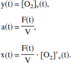
Equation 4 can now be cleanly rewritten as:

$\frac{\text{dy}}{\text{dt}}+\mathrm{a}(\mathrm{t})\cdot \mathrm{y}(\mathrm{t})=\mathrm{x}(\mathrm{t}).$

(6)

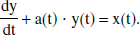
This linear inhomogeneous first-order differential equation is solvable by multiplying by the integrating factor exp(∫^t_t0a(s)ds), which allows Eq. 6 to be rewritten as

$\frac{\mathrm{d}}{\text{dt}}\left[\mathrm{y}\cdot \text{exp}\left({\int }_{{\mathrm{t}}_0}^{\mathrm{t}}\mathrm{a}(\mathrm{s})\text{ds}\right)\right]=\mathrm{x}\cdot \text{exp}\left({\int }_{{\mathrm{t}}_0}^{\mathrm{t}}\mathrm{a}(\mathrm{s})\text{ds}\right).$

(7)

Direct integration of Eq. 7 from t₀ to t yields

$\begin{array}{l}\mathrm{y}(\mathrm{t})\cdot exp\left({\int }_{{\mathrm{t}}_0}^{\mathrm{t}}\mathrm{a}(\mathrm{s})\text{ds}\right)-{\mathrm{y}(\mathrm{t}}_0)\cdot exp(0)\hfill \\ \hspace{0.17em}\hspace{0.17em}\hspace{0.17em}\hspace{0.17em}\hspace{0.17em}\hspace{0.17em}\hspace{0.17em}={\int }_{{\mathrm{t}}_0}^{\mathrm{t}}\mathrm{x}(\tau )\cdot \text{exp}\left({\int }_{{\mathrm{t}}_0}^{\mathrm{t}}\mathrm{a}(\mathrm{s})\text{ds}\right)\mathrm{d}\tau \text{.}\hfill \end{array}$

(8)

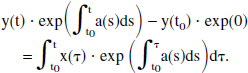
Therefore, the solution for y(t) is given by

$\begin{array}{lll}\mathrm{y}(\mathrm{t})\hfill & =\hfill & exp\left(-{\int }_{{\mathrm{t}}_0}^{\mathrm{t}}\mathrm{a}(\mathrm{s})\text{ds}\right)\cdot \left[{\mathrm{y}(\mathrm{t}}_0)+{\int }_{{\mathrm{t}}_0}^{\mathrm{t}}\mathrm{x}(\tau )\cdot exp\left({\int }_{{\mathrm{t}}_0}^{\mathrm{t}}\mathrm{a}(\mathrm{s})\text{ds}\right)\mathrm{d}\tau \right]\hfill \\ \hfill & =\hfill & \mathrm{y}({\mathrm{t}}_0)\cdot exp\left(-{\int }_{{\mathrm{t}}_0}^{\mathrm{t}}\mathrm{a}(\mathrm{s})\text{ds}\right)+{\int }_{{\mathrm{t}}_0}^{\mathrm{t}}\mathrm{x}(\tau )\cdot \text{exp}\left({\int }_{\mathrm{t}}^{\tau }\mathrm{a}(\mathrm{s})\text{ds}\right)\mathrm{d}\tau \text{.}\hfill \end{array}$

(9)

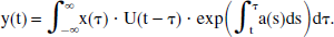
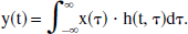
This expression is simplified even further by introducing the unit step function U(t), as well as by letting t₀ approach −∞, in which case the first term in Eq. 9 vanishes. Then, y(t) can be rewritten in the more compact form

$\mathrm{y}(\mathrm{t})={\int }_{-\infty }^{\infty }\mathrm{x}(\tau )\cdot \mathrm{U}(\mathrm{t}-\tau )\cdot exp\left({\int }_{\mathrm{t}}^{\tau }\mathrm{a}(\mathrm{s})\text{ds}\right)\mathrm{d}\tau .$

(10)

In a manner of speaking, y(t) describes the output of a linear system, with input function x(t) (Levan, 1987). Indeed, this conclusion follows logically from the linear differential equation (Eq. 6). Moreover, this “linear system” has a quasi-impulse response function of

$\mathrm{h}(\mathrm{t},\tau )=\mathrm{U}(\mathrm{t}-\tau )\cdot exp\left({\int }_{\mathrm{t}}^{\tau }\mathrm{a}(\mathrm{s})\text{ds}\right),$

(11)

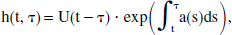
and therefore is not time-invariant, insofar as h(t, τ) is not a function of the difference t − τ. This function is called a “quasi-impulse response” inasmuch as it is not intrinsic to the system, but instead depends on part of the input itself (namely, the function a(t)). Even so, the valid superposition integral can still be written as follows:

$\mathrm{y}(\mathrm{t})={\int }_{-\infty }^{\infty }\mathrm{x}(\tau )\cdot \mathrm{h}(\mathrm{t},\tau )\mathrm{d}\tau .$

(12)

These conclusions should be taken with caution, because the terms under which this system may be called a linear one are very particular. Ideally, in the most general sense, the system should describe the cerebral physiologic response to task activation. Therefore, “input” should reflect the stimulus activation and “output” the cerebral response. At best, this model can describe only a single component of this system, with a single output of venous deoxyhemoglobin y(t) = [O₂]_v, and two inputs, which may be considered to be blood flow F(t) and oxygen consumption C′(t) (recall that the volume V(t), otherwise a third input, is kept constant in this model). Although these two input functions may be reasonable reflections of the more general “stimulus activation” input, several other “input pair” domains are certainly possible; for example, flow F(t) and extraction fraction E(t) could be used. However, the specific input function under which the system may be considered to be linear, once again, is x(t) (see italicized phrase above), which is a complex function of the two inputs F(t) and C′(t). To wit, using Eqs. 1 and 5, “transformation laws” can be found that describe how to shift between the two input domains(F(t),C′(t)) ↔ (a(t),x(t)):

$\begin{array}{lll}\mathrm{a}(\mathrm{t})\hfill & =\hfill & \frac{\mathrm{F}(\mathrm{t})}{\mathrm{V}},\hfill \\ \mathrm{x}(\mathrm{t})\hfill & =\hfill & \frac{\mathrm{F}(\mathrm{t})}{\mathrm{V}}\cdot {[{\mathrm{O}}_2{]}^{\prime }}_{\hspace{0.17em}\hspace{0.17em}\mathrm{v}}(\mathrm{t})=\frac{\mathrm{F}(\mathrm{t})}{\mathrm{V}}\cdot ({[{\mathrm{O}}_2]}_{\mathrm{a}}-\frac{{{\mathrm{C}}^{\prime }[\mathrm{O}}_2](\mathrm{t})}{\mathrm{F}(\mathrm{t})}).\hfill \end{array}$

(13)

The system is linear in the second domain, and then only with respect to its second input x(t). It is not linear in the first domain with respect to either input C′[O₂](t) or F(t), nor is it linear in the second domain with respect to its first input a(t).

Extended model.

The single differential equation used in the simple model (that is, Eq. 4) enables us to derive the form of the impulse response function; however, this simple model is incomplete in its handling of changes in cerebral blood volume (CBV or V). The balloon model of Buxton et al. (1997, 1998) provides an excellent mathematical framework to account for the role of cerebral blood volume using a system of coupled differential equations. In this section, the authors' simple model is extended to a similar set of coupled differential equations using the Buxton balloon hypotheses. The resulting system is, in fact, solved by essentially the same differential equation.

Briefly, Buxton proposed that the venous blood volume should be treated as a single well-mixed expandable compartment, similar to a passively distensible balloon, with a compliance curve specified by an exact equation such that the outflow is a function only of the volume. More precisely, rather than assigning a single flow function F, two functions F_in and F_out should be taken into consideration. These two functions, possibly different at any point in time, measure the flow into and out of the venous compartment. The time derivative of volume is then simply the difference between the inflow and outflow, and the function outflow = F_out(V) depicts a compliance curve, at any point of which the slope gives a measure of the elasticity of the balloon (that is, the reciprocal of its compliance). In other words, the above Eq. 3 should be amended to a system of two coupled differential equations:

${\mathrm{F}}_{\text{in}}(\mathrm{t})\cdot {[{\mathrm{O}}_2]}_{\mathrm{v}}^{\hspace{0.17em}\hspace{0.17em}\hspace{0.17em}\hspace{0.17em}\prime }-{\mathrm{F}}_{\text{out}}(\mathrm{t})\cdot {[{\mathrm{O}}_2]}_{\mathrm{v}}=\frac{\mathrm{d}}{\text{dt}}({[{\mathrm{O}}_2]}_{\mathrm{v}}\cdot \mathrm{V}(\mathrm{t})),$

(3a)

${\mathrm{F}}_{\text{in}}(\mathrm{t})-{\mathrm{F}}_{\text{out}}(\mathrm{t})=\frac{\text{dV}}{\text{dt}}.$

(3b)

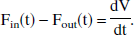
Here, Eq. 3a keeps track of total oxygen content in the venous compartment and 3b monitors its volume.

Now the product rule for derivatives is applied to Eq. 3a, thereby combining these two equations to derive

$\begin{array}{l}{\mathrm{F}}_{\text{in}}(\mathrm{t})\cdot {[{\mathrm{O}}_2]}_{\mathrm{v}}^{\hspace{0.17em}\hspace{0.17em}\hspace{0.17em}\prime }-{\mathrm{F}}_{\text{out}}(\mathrm{t})\cdot {[{\mathrm{O}}_2]}_{\mathrm{v}}=\frac{\mathrm{d}}{\text{dt}}({[{\mathrm{O}}_2]}_{\mathrm{v}}\cdot \mathrm{V}(\mathrm{t}))\hfill \\ \hspace{0.17em}\hspace{0.17em}\hspace{0.17em}\hspace{0.17em}\hspace{0.17em}\hspace{0.17em}\hspace{0.17em}\hspace{0.17em}\hspace{0.17em}\hspace{0.17em}\hspace{0.17em}={[{\mathrm{O}}_2]}_{\mathrm{v}}\cdot \frac{\text{dV}}{\text{dt}}+\mathrm{V}(\mathrm{t})\cdot \frac{\mathrm{d}}{\text{dt}}{[{\mathrm{O}}_2]}_{\mathrm{v}}\hfill \\ \hspace{0.17em}\hspace{0.17em}\hspace{0.17em}\hspace{0.17em}\hspace{0.17em}\hspace{0.17em}\hspace{0.17em}\hspace{0.17em}\hspace{0.17em}\hspace{0.17em}\hspace{0.17em}={[{\mathrm{O}}_2]}_{\mathrm{v}}\cdot ({\mathrm{F}}_{\text{in}}-{\mathrm{F}}_{\text{out}})+\mathrm{V}(\mathrm{t})\cdot \frac{\mathrm{d}}{\text{dt}}{[{\mathrm{O}}_2]}_{\mathrm{v}},\hfill \end{array}$

which implies

${\mathrm{F}}_{\text{in}}(\mathrm{t})\cdot {[{\mathrm{O}}_2]}_{\mathrm{v}}^{\hspace{0.17em}\hspace{0.17em}\hspace{0.17em}\hspace{0.17em}\prime }-{\mathrm{F}}_{\text{in}}(\mathrm{t})\cdot {[{\mathrm{O}}_2]}_{\mathrm{v}}=\mathrm{V}(\mathrm{t})\cdot \frac{\mathrm{d}}{\text{dt}}{[{\mathrm{O}}_2]}_{\mathrm{v}}.$

(3c)

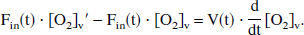
Therefore, comparing Eq. 3c with Eq. 4, it can be seen that the solution to this system of two differential equations is equivalent to that already derived for the simple model, with F replaced by the F_in function and the constant V now replaced by a function V that varies in time. (Actually, in their article, Buxton et al. studied the deoxyhemoglobin curve rather than oxyhemoglobin, but this difference does not significantly alter the above argument.)

Two noteworthy points may be deduced from the above equations. First, Eq. 3b may be solved to find V(t) in a manner completely independent of the solution of Eq. 3a or 3c. This conclusion makes sense, because the oxygen content of the venous pool should have no effect on its changes in volume in the model presented here. In a sense, the volume curve V(t) can therefore be treated as a second output of the extended model, and the solution for V(t) depends on the input F_in(t) and even more on the compliance curve F_out(V). The assumed form of this compliance curve will be addressed in more detail below. Second, and similarly, the outflow F_out curve can be noted to have no direct bearing on the solution of Eq. 3c, other than by its effect on V(t). Therefore, in theory, these “coupled” differential equations may in fact be solved one at a time—first for V(t), and then for y(t).

RESULTS

Using “reasonable” curves for the inputs—oxygen consumption C′ (t) and blood flow F(t)—simulations are performed using Eq. 6, solving for the output function y = [O₂]_v. The first three sections document the simulations that test the authors' models, the first two testing the simple model in a similar fashion to the investigations of Boynton et al. (1996) and Dale and Buckner (1997), respectively. The third section reapplies these two tests to the extended model, with a volume parameter varying according to Buxton's (1998) balloon model equations. When possible, functions are modeled using known physiologic parameters within the context of the respective experiment simulations. These simulations were performed on a Macintosh using the Matlab (MathWorks, Natick, MA, U.S.A.) software package.

In the computations that follow, even though a closed integral form of y(t) is given above, in practice the authors resorted to solving the underlying differential equation. In other words, rather than use the integral Eq. 9 or 12, they used an iterative second-and third-order Runge-Kutta method to solve Eq. 6. There are several reasons for this practice. First, the Matlab software package has prewritten routines for solving coupled differential equations with high speed and precision, whereas the integral solution is somewhat more burdensome and time-consuming. Also, in previous work, the authors found that the two methods yield no significant difference in their results (Hathout et al., 1995), and thus are computationally equivalent.

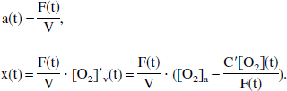
To solve Eq. 6, formulas for a(t) and x(t) are needed. Following other investigators' lead, one solves in terms of normalized functions with unit baseline (Buxton et al., 1998). The solution for a(t) follows from its definition, given in Eq. 5:

$\mathrm{a}(\mathrm{t})=\frac{\mathrm{F}(\mathrm{t})}{\mathrm{V}(\mathrm{t})}=\left(\frac{{\mathrm{F}}_0}{{\mathrm{V}}_0}\right)\cdot \left(\frac{\mathrm{f}(\mathrm{t})}{\mathrm{v}(\mathrm{t})}\right),$

(14)

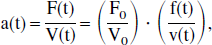
where the lowercase variables f and v denote normalized quantities and the baseline values are subscripted with zero. To solve for x(t), one starts with the definition of extraction fraction E(t) = 1 − [O₂]′_v/[O₂]_a, which can be solved for [O₂]′_v:

${[{\mathrm{O}}_2]}_{\hspace{0.17em}\hspace{0.17em}\mathrm{v}}^{\prime }={[{\mathrm{O}}_2]}_{\mathrm{a}}\cdot (1-\mathrm{E}(\mathrm{t}))\text{.}$

(15)

If the assumption of constant consumption is invoked, then the quantity E(t) · F(t) is a constant (see Eq. 2). Then, one may write E(t) = E₀/f(t), and so

${[{\mathrm{O}}_2]}_{\hspace{0.17em}\hspace{0.17em}\mathrm{v}}^{\prime }={[{\mathrm{O}}_2]}_{\mathrm{a}}\cdot (1-{\mathrm{E}}_0/\mathrm{f}(\mathrm{t}))\text{.}$

(16)

Combining Eq. 16 with the definition of x, again from Eq. 5, it is found that

$\mathrm{x}(\mathrm{t})=\left(\frac{{\mathrm{F}}_0}{{\mathrm{V}}_0}\right)\cdot \left(\frac{\mathrm{f}(\mathrm{t})}{\mathrm{v}(\mathrm{t})}\right)\cdot {[{\mathrm{O}}_2]}_{\mathrm{a}}\cdot (1-{\mathrm{E}}_0/\mathrm{f}(\mathrm{t}))\text{.}$

(17)

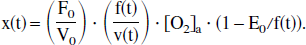
Finally, one assumes that one is starting from an equilibrium state where dy/dt = 0, so that y = [O₂]_v and [O₂]′_v would have the same baseline value (by Eq. 4), which must therefore equal y₀ = [O₂]_a · (1 − E₀) (by Eq. 15). Putting it all together, if $\bar{\mathrm{y}}=\mathrm{y}/{\mathrm{y}}_0$ is allowed to denote the normalized version of y = [O₂]_v, then Eq. 6 can be rewritten as

$\begin{array}{lll}\frac{\mathrm{d}\bar{\mathrm{y}}}{\text{dt}}\hfill & =\hfill & \left(\frac{\mathrm{x}(\mathrm{t})-\mathrm{a}(\mathrm{t})\cdot \mathrm{y}(\mathrm{t})}{{\mathrm{y}}_0}\right)\hfill \\ \hfill & =\hfill & \left(\frac{{\mathrm{F}}_0}{{\mathrm{V}}_0}\right)\cdot \left(\frac{\mathrm{f}(\mathrm{t})}{\mathrm{v}(\mathrm{t})}\right)\cdot \left(\frac{1-{\mathrm{E}}_0/\mathrm{f}(\mathrm{t})}{1-{\mathrm{E}}_0}-\bar{\mathrm{y}}\right).\hfill \end{array}$

(18)

Interestingly, the solution for the normalized function $\bar{\mathrm{y}}(\mathrm{t})$ therefore depends on four quantities, two constant and two variable: the initial extraction fraction E₀, the initial flow/volume ratio F₀/V₀, and the two normalized functions f(t) and v(t). The authors' software program solves for $\bar{\mathrm{y}}(\mathrm{t})$ iteratively, given these four quantities.

In the first two sections, the authors used an initial flow/volume ratio of F₀/V₀ = 0.15 sec⁻¹ and an initial extraction fraction E₀ = 0.32, in keeping with known measured values (Hathout et al., 1995). A stimulus pulse is modeled as a symmetric trapezoidal envelope in blood flow F(t), where activation begins at time = 1 second. The rise and decline times occur over 3 seconds (Ogawa et al., 1993), and the total time between stimulus onset and fall of the input function measures the duration of the pulse. For example, a 12-second pulse consists of a 3-second rise, a 9-second plateau, and then a 3-second decline. The height of the input function was also chosen to correspond to known physiologic parameters. In the positron emission tomography study by Fox and Raichle (1986) studying the somatosensory cortex, blood flow was found to increase by approximately 30%. The maximal flow at the plateau was therefore initially taken to be 1.3, where baseline flow is 1.0.

Reconstructing the fMRI response from a linear summation of time-shifted responses to pulses of shorter duration

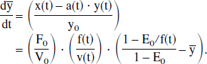
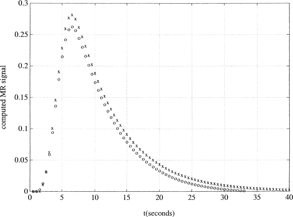
Recreating the experiment of Boynton et al. (1996), the simple model was first used to compute the output function y = [O₂]_v using input functions corresponding to 3-, 6-, and 12-second pulses. The response to a 12-second pulse was compared with a linear summation of the time-shifted responses to two 6-second pulses, as well as to the similar sum of four 3-second pulses. These three curves are shown simultaneously in Fig. 1.

FIG. 1.

Prediction of the functional magnetic resonance imaging signal response to a 12-second pulse from linear summations of shorter time-shifted pulse responses. The venous oxygenation response to a 12-second pulse (open circles) is compared with the calculated 12-second response obtained by summing two 6-second pulse responses, appropriately shifted in time (*), as well as a similar sum of four 3-second pulse responses (x). There is a progressive overshoot during the activation phase as shorter pulse responses are used to predict responses to longer stimuli. This overshoot persists in the postactivation phase.

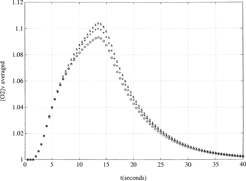
The open circles show the response to the 12-second pulse. There is a slow increase in venous oxygen concentration from baseline to its peak, demonstrating the lag between stimulus onset and peak response (Hathout et al., 1995). The venous concentration then declines as expected back to baseline. The asterisks represent the summed responses to two 6-second pulses, beginning at 0 and 6 seconds, respectively. The × symbols similarly depict the summed response reconstructed from four 3-second pulse responses, shifted in time by 0, 3, 6, and 9 seconds. For comparison, Fig. 2 is adapted from the work of Boynton et al. (1996), with the thin curve depicting the time-shifted sum of four 3-second pulse responses and the bold curve representing the fMRI signal response to a 12-second stimulation.

FIG. 2.

Empirical results from the work of Boynton et al., (1996) where 4 time-shifted 3-second pulse responses (thin curve) were used to estimate the functional magnetic resonance imaging (fMRI) signal response to a 12-second visual stimulation pulse (thick curve). The horizontal axis is time in seconds, and the vertical axis is fMRI signal units. Reprinted with permission from GM Boynton, SA Engel, GH Glover, DJ Heeger (1996) Linear systems analysis of functional magnetic resonance imaging in human V1. J Neurosci 16(13):4207–4221.

The figures are similar in several respects, although they are not a perfect match. In both figures, there is close agreement between the two summed responses and the original 12-second curve, demonstrating near-linear behavior. In addition, during the activation phase of both figures, both summed responses are noted to overestimate the 12-second pulse response slightly, and this phenomenon is systematic in that the four 3-second pulse reconstruction produces a slightly greater overshoot than the two 6-second pulses (this phenomenon was also evident in Boynton's results, not shown in Fig. 2). However, in the postactivation phase, a failure is noted in the predictions of the simple model. Experimentally, the summed response produces an undershoot in this late phase, which is not predicted by the simulations. This point will be readdressed below, where it will be found that the extended model can correct this deficiency.

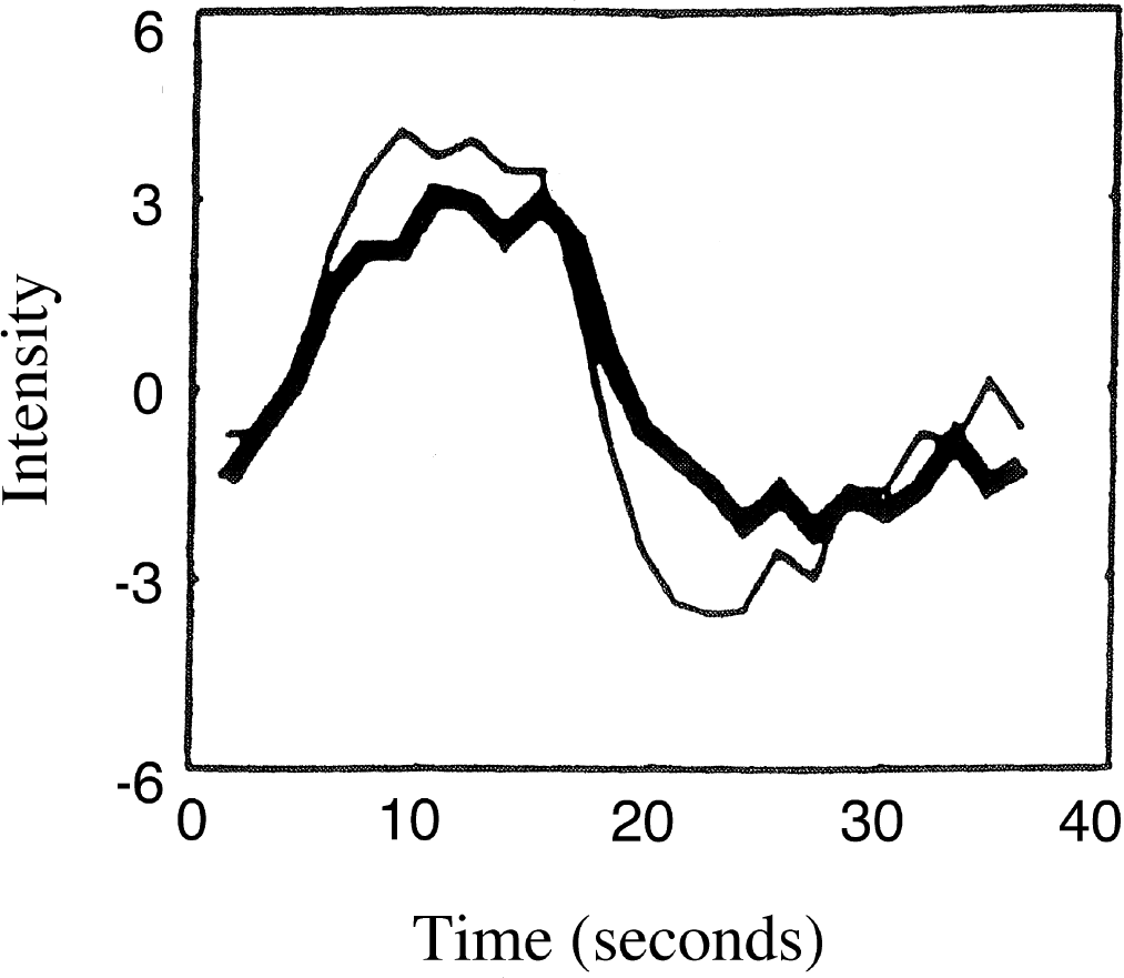
To test the robustness of these predictions, the authors ran the simulations again with different parameters (Fig. 3). The rise time of the trapezoidal envelope was allowed to be 2 or 3 seconds, and the maximal flow was allowed to be 1.3, 1.5, or even 1.7, relative to baseline. Allowing these parameters to vary did not substantially change the conclusions: during the activation phase, the summed four 3-second curves always yielded an overestimate of the summed two 6-second curves, which similarly overestimated the 12-second curve. Therefore, the predictions are robust across several physiologic choices of parameter values.

FIG. 3.

Testing the robustness of conclusions with respect to different parameter choices. Venous oxygenation responses to 12-second pulses (open circles), compared with the computed responses by summing 3-second pulses (x), are displayed for different parameter choices by varying either the rise time (2 or 3 seconds) or the maximal flow amplitude (30%, 50%, or 70%). (A) 3-second rise, 30% maximum flow;(B) 2-second rise, 30% maximum flow;(C) 3-second rise, 50% maximum flow;(D) 3-second rise, 70% maximum flow. The overshoot is observed across all parameter choices, although its magnitude varies.

Separating individual pulse responses in a two-trial cluster

The experiment of Dale and Buckner (1997) was recreated as follows. Each single trial was modeled as a short pulse (3 seconds in duration). The two-trial cluster consisted of two 3-second pulses, whose initial times were separated by 7 seconds. Once again, blood flow was assumed to increase by 30% over 3 seconds, and the first activation began at time = 1 second.

Figure 4A displays the output functions y = [O₂]_v using either the one-or two-trial cluster as input. The response to the two-trial cluster reached a higher peak than the one-trial cluster, illustrating the phenomenon of an additive hemodynamic response (Boynton et al., 1996). In Fig. 4B, the × symbols graph the response to a single-trial input, and the open circles show the net difference signal (the single-trial response subtracted from the two-trial response), shifted backward in time by 7 seconds, which is the separation between the two trials.

FIG. 4.

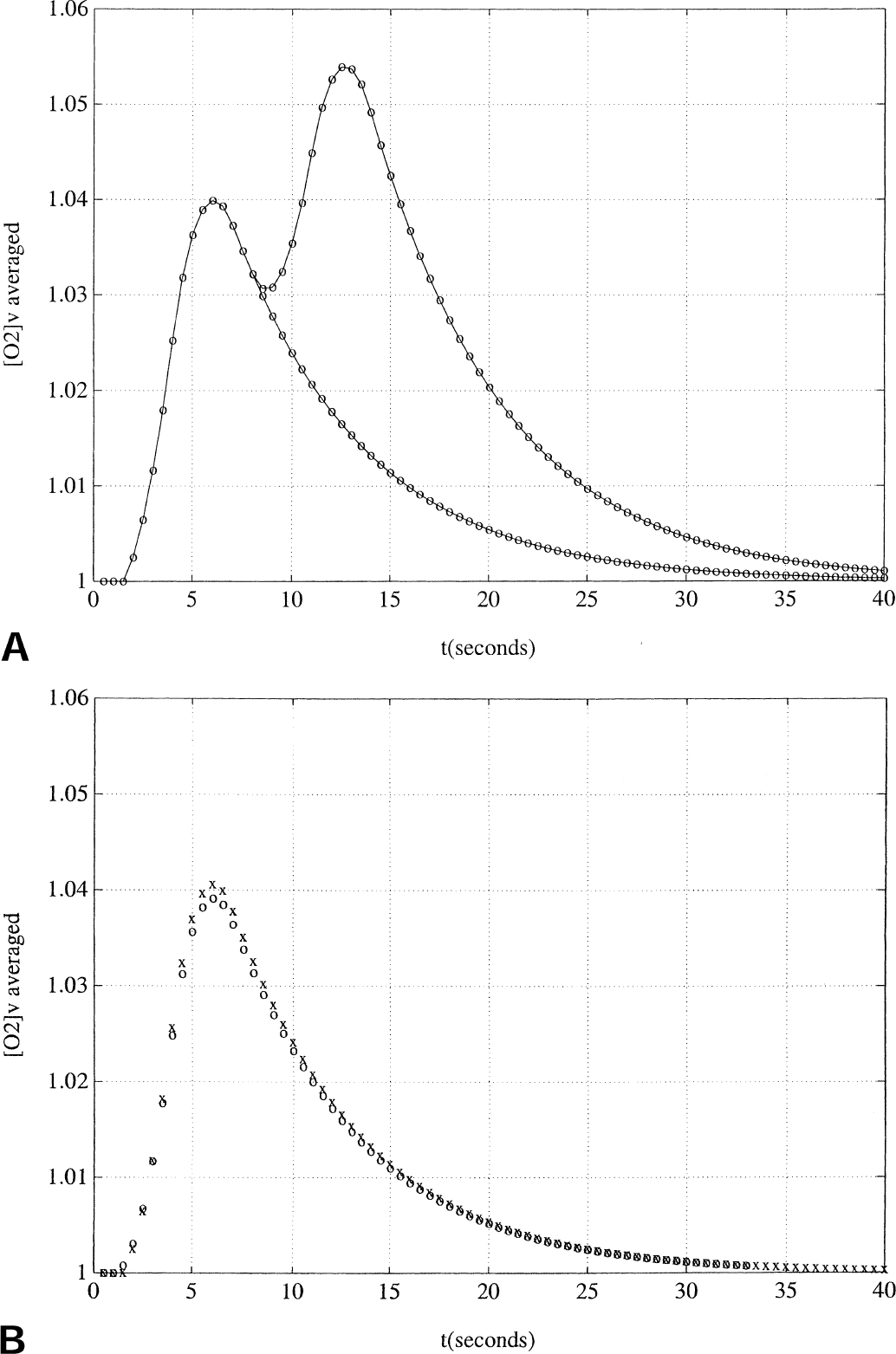
Predicting individual pulse responses from a two-trial cluster. (A) Calculated venous oxygenation in response to a two-pulse cluster using two 3-second pulses, separated by 7 seconds; superimposed is the calculated response to a single 3-second pulse. (B) The calculated contribution of the second pulse (open circles) is obtained by first subtracting the response to a single pulse from the two-pulse cluster, and then by shifting backward in time by 7 seconds. It is compared with the single-pulse response (x). The calculated contribution of the second pulse slightly undershoots the single-pulse response, but this undershoot diminishes during the declining phase.

At first glance, a close match is found between the single-trial response and the time-shifted difference signal, which in theory represents the calculated isolated response to the second trial. This close approximation demonstrates consistency with the hypotheses of linearity and time-invariance and duplicates the empirical results of Dale and Buckner (1997). Comparable graphs from their paper are shown in Fig. 5. More interestingly, the slight but definite undershoot by the calculated second-trial response is also reproduced by the model, although less pronounced than what is found experimentally. Therefore, as in the results from the Boynton simulations above, the simple model predicted the near-linearity of the cerebral response and also accounted partly for the nature of the subtle departures from LTI behavior. Tests of robustness across multiple parameter values, similar to those performed in the first section, again found no substantial difference in these findings: the near-linearity held true.

FIG. 5.

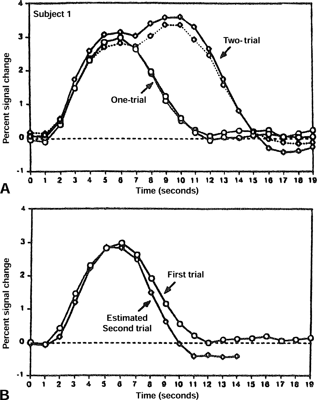
Predicting individual pulse responses from a two-trial cluster: the empirical data of Dale and Buckner (1997). (A) Percentage signal change with a two-pulse cluster compared with a single pulse. (B) Estimated response to the second pulse, undershooting the single-pulse response. Reprinted from AM Dale, RL Buckner (1997) Selective averaging of rapidly presented individual trials using fMRI. Human Brain Mapping 5:329–440, with permission from Wiley-Liss, Inc., a subsidiary of John Wiley & Sons, Inc.

On closer inspection, a slight failure of the simple model is found. The undershoot of the calculated difference signal in the declining phase is not completely reproduced in the authors' simulation; indeed, the simple model appears to predict that the two curves should reapproach each other during the declining phase (Fig. 4B). As before, in the next section, it will be discovered that the extended model can correct this deficiency as well, because it can reproduce even this subtle finding.

Simulations using the extended balloon model

In applying the extended balloon model, the authors again used a trapezoidal flow-time curve to represent a stimulus pulse, with rise and fall times of 3 seconds and maximal height of 30% increase from baseline. As noted above, computation of the function V(t), now varying in time, depends heavily on the compliance curve F_out(V). Grubb et al. (1974) experimentally found that the end points of this curve should roughly obey the power law relationship v = f^0.4, where again lowercase letters denote the corresponding normalized functions whose baseline values are 1.0. Therefore, with the assumption of the flow increasing 30% with task activation, one can specify two end points of the normalized compliance curve: f_out(1) = 1 and f_out(1.3^0.4) = 1.3. The shape of the intervening curve is not known, although Buxton et al. (1998) ran their simulations based on different forms of the curve: linear, convex nonlinear, as well as one with a small hysteresis between balloon inflation and deflation. In contrast, Glover (1999) used a nonlinear curve that is concave.

Not surprisingly, the predictions of the simulations are found to vary widely with the shape of this compliance curve. Glover (1999) modeled F_out as the sum of a linear component and a power law; in other words, f_out is of the form:

${\mathrm{f}}_{\text{out}}(\mathrm{v})=1+{\lambda }_1\cdot (\mathrm{v}-1)+{\lambda }_2\cdot {(\mathrm{v}-1)}^{\alpha }.$

(19)

In the authors' simulations, they chose Buxton et al.'s third curve with the hysteresis—that is, the flow-volume curve changes between balloon inflation and deflation. As pointed out in that article, this curve models a balloon that is initially stiff but becomes more compliant with prolonged expansion. For deflation from an initial state (v₁,f₁), the authors used the same convex curve used by Glover, with α = 3, λ₁ a chosen parameter, and λ₂ computed to satisfy the end point condition f_out(v₁) = f₁. For inflation from an initial state (v₂,f₂), the authors used the rotationally symmetric concave curve given by

${\mathrm{f}}_{\text{out}}(\mathrm{v})={\mathrm{f}}_{\text{max}}-{\lambda }_1\cdot ({\mathrm{v}}_{\text{max}}-\mathrm{v})-{\lambda }_2*\cdot {({\mathrm{v}}_{\text{max}}-\mathrm{v})}^{\alpha }$

(20)

where f_max denotes the maximal flow, v_max = (f_max)^0.4 the volume at maximal flow, and λ₂* is again computed from the end point condition f_out(v₂) = f₂. At baseline, the authors therefore started at the state (v,f) = (1,1). For the single-pulse activation simulations, the balloon underwent only one round each of inflation and deflation; for the double-pulse activations in recreating Dale and Buckner's experiments, there were two of each.

By allowing the creation of a volume variable, the authors enabled one additional refinement to be made: the transition of output from venous deoxygenation to fMRI signal. As mentioned before, the models presented so far can describe only one component of the complex human cerebral system that translates a given task activation into a measurable fMRI signal. In the simple model, the input is regional blood flow, F(t), and the only output is venous oxyhemoglobin, y = [O₂]_v, in which place one may just as easily use venous deoxyhemoglobin if so desired. In the extended model, the authors in effect have a second output of venous volume V(t). In their recent work on the balloon model, Buxton et al. (1998) derived a theoretical expression for BOLD MR signal that depends on these two functions:

$\frac{\Delta \mathrm{S}}{\mathrm{S}}={\mathrm{V}}_0\cdot \left[{\mathrm{k}}_1\cdot (1-\mathrm{q})+{\mathrm{k}}_2\cdot \left(1-\frac{\mathrm{q}}{\mathrm{v}}\right)+{\mathrm{k}}_3\cdot (1-\mathrm{v})\right],$

(21)

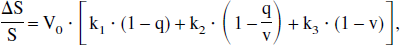
where q represents normalized deoxygenated hemoglobin content and the constants k₁ = 7 E₀, k₂= 2, k₃ = 2 E₀ − 0.2 are estimated using measured values of the intravascular and extravascular signal components of the MR signal.

Casual inspection of this formula reveals how large an effect the volume-time curve can have on the magnitude of the BOLD signal. With the volume held constant, as in the simple model, the signal-time curve and the oxyhemoglobin-time curve roughly parallel one another. But when allowed to vary as in the extended model, the volume curve exerts a second independent influence on the MR signal-time curve. In the results that follow on the extended model, therefore, this expression will be used for BOLD signal rather than venous deoxyhemoglobin as a more accurate representation of the system output.

Currently, there is no consensus on the appropriate form of the flow-volume envelope, and different authors have used significantly different parameters (Buxton et al., 1998; Glover, 1999). After running multiple simulations using different forms of the flow-volume compliance curve, the authors found that even slight changes in this curve (or curves with hysteresis) can result in significant changes in the resulting MR signal-time curve. The results presented here use the hysteresis curves, as modeled above, using λ₁ = 0.1 and 0.5. In support of this choice, the authors note that Buxton et al., in simulations using similar flow-volume curves with hysteresis, found results that could duplicate the initial overshoot and the poststimulus undershoot of the fMRI signal, phenomena that have been well documented empirically in multiple reports (Frahm et al., 1996; Kruger et al., 1998, 1999).

Where Buxton used an initial E₀ of 0.4, the authors continued to use the value of 0.32, as before. Buxton used an initial flow/volume ratio of 0.5 sec⁻¹, whereas the authors believe that the value of 0.15 sec⁻¹ used in this article has more physiologic grounding (Hathout et al., 1995; Leenders et al., 1990). As a further difference, the authors' model assumed a constant rate of oxygen consumption; Buxton et al. derived a formula that links oxygen extraction to blood flow (Buxton and Frank 1997; Buxton et al., 1998).

Figures 6 and 7 display the results with the simulations under the assumptions of the extended model, with a volume function that was allowed to vary in time. For Fig. 6, the Boynton experiment recreations, the authors used a flow-volume envelope specified by the parameter of λ₁ = 0.1. In Fig. 7, for the Dale and Buckner simulation, the results are displayed with λ₁ = 0.5. The extended physiologic model still succeeded in predicting both the near-linear behavior found in the first two simulations, as well as the gross nature of the slight deviations from it. In other words, the main deviations from the LTI model found in Boynton's experiments (the overestimation by the summated reconstructed signal during the activation phase) as well as those in Dale and Buckner's (the underestimation by the computed difference signal) were both still observed.

FIG. 6.

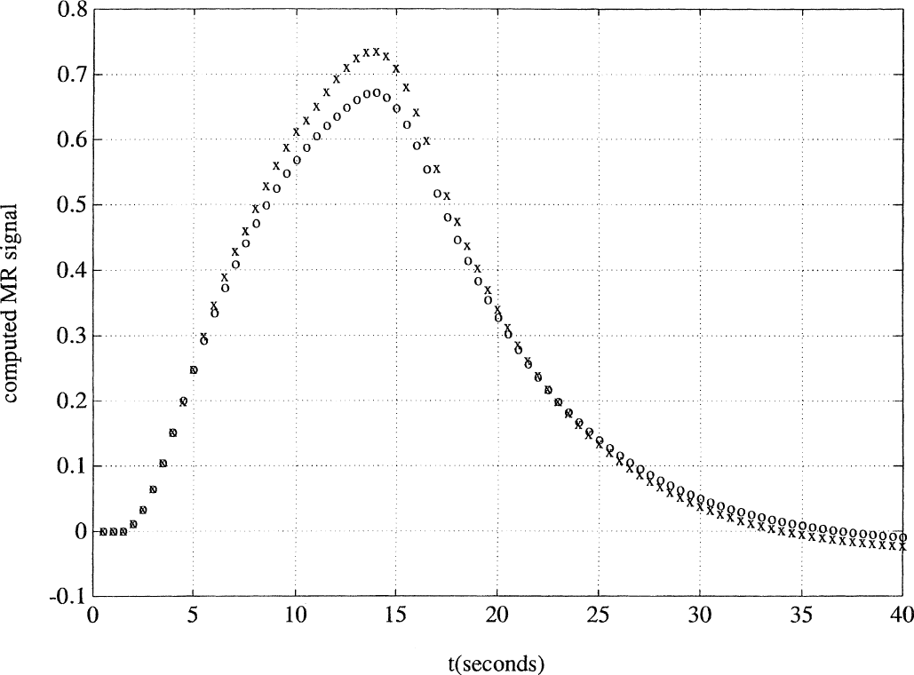
Comparison of the change in computed functional magnetic resonance imaging signal response with a 12-second pulse (open circles) versus the predicted response from summing 4 time-shifted 3-second pulse responses (x) using an extended model similar to Buxton's balloon model, with hysteresis curves specified by λ₁ = 0.1. The results are a better qualitative match with Boynton's empirical data, showing both the activation phase overshoot and the postactivation undershoot.

FIG. 7.

Predicting individual pulse responses from a two-trial cluster using the extended model similar to Buxton's balloon model, λ₁ = 0.5. Once again, there is a better match with the empirical data: the calculated signal response from the second pulse (open circles) slightly undershoots the time-shifted single-pulse response (x), and this undershoot persists throughout the declining phase.

However, closer inspection of the figures shows that the extended model succeeded better where the simple model failed. In the Boynton simulation, the summed MR signal curve from the four 3-second pulses duplicated the undershoot of the 12-second signal response during the postactivation phase, a finding that was not predicted by the simple model. Moreover, in the Dale and Buckner simulation, the persistent undershoot throughout the declining phase was better duplicated in the extended model, whereas the simple model mistakenly predicted that this undershoot would diminish during the declining phase.

Now that the output function is expressed in terms of MR signal, one may attempt to quantify how well the extended model accounts for the extent of the measured nonlinearities in the two respective articles. For Boynton, the authors estimated the overshoot of the predicted summated curve, using four 3-second pulses, to be approximately 30% of the full height of the actual 12-second curve (Fig. 2). Because no numeric data were presented in their work, this quantity can only be estimated from their figures. In the authors' simulation, the overshoot amounted to only 12%, showing that this simulation did not fully account for the measured nonlinearity (Fig. 6). Similarly, the magnitude of the postactivation undershoot, in both the summated curve and the actual 12-second curve, was clearly underestimated by the authors' simulations.

Quantifying the results for the Dale and Buckner simulation is more difficult because the undershoot manifests only as a very slight decrease in the declining phase. If the full-width at half-maximum is measured, the predicted isolation of the second pulse response has approximately 90% of the width of the original pulse. Comparable measurements from a figure in Dale and Buckner's (1997) article show that the estimated second pulse has 83% of the width of the first pulse (Fig. 5). Once again, although the authors' simulations did capture the qualitative discrepancies of the experiment, they fell short of a full quantitative explanation.

DISCUSSION

The field of fMRI has become increasingly sophisticated during the past decade, probing ever more subtle aspects of cerebral physiology and the relationship between stimulus-induced cortical activation and the resultant fMRI signal. An important research area in this vein has been event-related fMRI and the closely related investigations of fMRI signals in the context of linear systems analysis (Boynton et al., 1996; Buckner et al., 1996; Dale and Buckner, 1997; Friston et al., 1998; Glover, 1999; Rosen et al., 1998).

Currently, the elegance of fMRI task paradigms is often limited by the need to use repetitions of blocked tasks or activation stimuli to obtain sufficient signal-to-noise ratios to generate fMRI images (Dale and Buckner, 1997). Methods that allow the separation of individual pulse responses (task responses) in the fMRI signal would allow the use of much more sophisticated mixed-task paradigms (Dale and Buckner, 1997). The achievement of such methods requires an understanding of both the temporal evolution of the fMRI signal to individual tasks (event-related fMRI) and the development of adequate systems modeling of the fMRI signal as a function of individual pulse responses (Boynton et al., 1996; Buckner et al., 1996; Dale and Buckner, 1997; Friston et al., 1998; Glover, 1999; Rosen et al., 1998). With such an understanding, it becomes possible in some instances to deconvolve the fMRI pulse response of individual tasks in a multistimulus paradigm (Friston et al., 1998; Glover, 1999).

An intrinsic difficulty in such a deconvolution, or the separation of individual fMRI pulse responses, is the fact that the fMRI signal is “heavily filtered by the hemodynamic delay inherent in the BOLD contrast mechanism, and therefore temporally evolving events are blurred” (Glover, 1999). With cortical activation, an excess of flow over oxidative metabolism leads to decreased end-capillary deoxyhemoglobin levels, which then wash into the venules and eventually alter the regional venous deoxyhemoglobin levels (Buxton and Frank, 1997; Hathout et al., 1995). This leads to delayed temporal evolution of the fMRI signal relative to neuronal activaiton. Prior mass-balanced models of cerebral blood flow and oxygen consumption have shown some accuracy in characterizing these delays and the shape of the fMRI signal envelope (Buxton et al., 1998; Hathout et al., 1999).

In this article, physiologic modeling was used in a systems analysis of fMRI signals. Thus far, several investigators have shown that fMRI signal responses can be roughly characterized by assuming an LTI system, (Boynton et al., 1996; Dale and Buckner, 1997) and this paradigm has been the basis for most event-related fMRI modeling (Boynton et al., 1996; Buckner et al., 1996; Dale and Buckner, 1997; Friston et al., 1998). Although such linear models have been relatively successful, some deviations from linearity have been noted with visual fMRI experiments (Boynton et al., 1996; Dale and Buckner, 1997) as well as with auditory stimulus response experiments (Robson et al., 1998). More profound nonlinearities and the need for more sophisticated analysis paradigms have been shown for short-duration stimuli in visual, auditory, and sensorimotor cortex (Friston et al., 1998; Glover, 1999; Vazquez and Noll, 1998).

In the current study, the authors reexamined a simple mathematical model of cerebral vascular physiology in the light of the results of two recent articles and extended the model along the lines of a model presented in a third. In the publications by Boynton et al. (1996) and Dale and Buckner (1997), empirical data were shown to be roughly consistent with an LTI system, which was then further characterized using a parametrized impulse response function. The simple model presented in this article and the extended model incorporating the equations of Buxton et al. for handling volume changes both build on these interesting results in several ways. Because they are both derived from physiologic assumptions, the models are potentially more illuminating than a mere parametric analysis.

More importantly, both models nicely match the empirical results seen in the two articles. They successfully predict the approximate LTI behavior as seen by Boynton et al., who reconstructed the fMRI signal response to a long pulse by summating the signal response to shorter pulses. The simple model also qualitatively predicts the mild overshoot of the predicted summed pulse response during the activation phase, and the extended model further predicts the postactivation undershoot.

Similarly, the nearly linear behavior of the fMRI signal response in Dale and Buckner's work and the subtle deviations from linearity are also well shown by the authors' models. The predicted response to the isolated second stimulation pulse in a two-trial cluster nearly matches a time-shifted copy of the fMRI response to a single pulse, consistent with a linear system. Moreover, the slight undershoot of the predicted second pulse response compared with the single pulse-response is also predicted: grossly by the simple model, and more accurately by the extended model.

Although mere consistency with empirical data does not by any means constitute a proof of these models, it does provide at least indirect support of the authors' simulations as a useful model of fMRI physiology. The data are also consistent with the BOLD hypothesis for fMRI signal formation, because the output function of venous oxyhemoglobin in the simple model had some success in predicting the empirical results. Moreover, these models provide a putative explanation for the nearly linear behavior of fMRI signal response (similar to the predictions of parametric LTI models) but go beyond such models in also predicting the empirically observed subtle deviations of fMRI signal from ideal LTI behavior, and possibly shedding light on the source and nature of the nonlinearities.

Indeed, an analysis of the equations underlying the simple physiologic model reveals the source of its near-linearity with respect to cerebral blood flow and therefore may provide some insight into the near-linearity of the more complex system representing the fMRI response to task activation. Recall that the output function y(t) does in fact vary linearly with an input function x(t), which is a combined function of the two inputs, F(t) and C′ (t), given by Eq. 13:

$\mathrm{x}(\mathrm{t})=\frac{\mathrm{F}(\mathrm{t})}{\mathrm{V}}\cdot \left({[{\mathrm{O}}_2]}_{\mathrm{a}}-\frac{{\mathrm{C}}^{\prime }[{\mathrm{O}}_2](\mathrm{t})}{\mathrm{F}(\mathrm{t})}\right).$

We can rewrite this in terms of the extraction fraction using Eq. 2:

$\mathrm{x}(\mathrm{t})=\frac{\mathrm{F}(\mathrm{t})}{\mathrm{V}}\cdot {[{\mathrm{O}}_2]}_{\mathrm{a}}\cdot (1-\mathrm{E}(\mathrm{t}))\text{.}$

Therefore, to the extent that the first input factor F(t) predominates over the second input factor (1 − E(t)), the complex input function will roughly track the blood flow F(t). For instance, in the authors' simulations, the blood flow rises 30% in task activation. With constant oxygen consumption, the factor (1 − E) increases by only 11%. Therefore, the contribution from flow predominates, and the input function x(t), under which the system is linear, closely tracks the flow function F(t). This explains the approximately linear behavior of the simple model with respect to this input.

However, because the model is inherently nonlinear with respect to cerebral blood flow, it may also help elucidate the empirically observed deviations from linearity, which defy characterization within an LTI framework, and so may suggest some of the reasons underlying the more profound nonlinearities noted by other authors. At very short stimulation bursts, there is probably a minimal threshhold for cerebral increases in blood flow (a sort of cerebral quantum response), where shorter or more subtle stimulation cannot elicit even less of a cerebral blood flow response. Either it would elicit no response or the minimal quantum of response, and no linear relationship between stimulus duration or intensity and fMRI signal would be present in these ultrashort or low-intensity stimulation paradigms. This notion seems consistent with some of the data presented in this field, such as the work of Vasquez and Noll (1998). In that work, fMRI signal responses to visual stimulation <4 seconds in duration and <40% contrast yielded strong nonlinear responses. At this time, however, there are no reliable data on how to model such a minimal quantum response.

In a qualitative sense, the authors' models successfully describe the nonlinearities observed in the articles by Boynton et al. and Dale and Buckner. From the quantitative data, one may conclude that this description is incomplete, so that additional nonlinearities must be present in these experiments. As stated before, the simple model and even the extended model at best can describe only a small component of the more general system in question—namely, the system of cerebral fMRI response to task activation. In theory, this more general system may be considered as a series of three input/output systems in tandem, the output of one serving as the input to the next. The first such postulated system would accept as input the task activation process and would produce as output the hemodynamic responses within the brain, as dictated by the metabolic demands of increased neuronal activity. These outputs might include increased cerebral blood flow, blood volume, and oxygen consumption. A second system would accept these physiologic outputs as its input and produce as its output the salient characteristics describing the internal composition of the brain, such as venous deoxyhemoglobin content. The third system would then translate these internal characteristics into a measurable fMRI signal.

Clearly, the models presented here attempt to model only the second system in this chain. The first and third systems remain as black boxes whose inner workings remain largely a mystery, although Buxton et al. (1998) attempted a theoretical derivation of fMRI signal that was used in the current article. One may almost certainly assume that each subsystem contains the additional nonlinearities unaccounted for in the authors' models quantitatively. Even the inner workings of this second subsystem are far from apparent—for example, little is known about the proper shape of the compliance curve describing the mechanical distensibility of the venous compartment. The current investigations suggest that the hysteresis model may have some validity, given its predictive success in duplicating the finer deviations from linearity presented here. Further attempts to elucidate the inner workings of all three of these black boxes should be a focus of future research. The importance of these pursuits is made all the more pressing by the increasing number of fMRI experiments using task-activation paradigms that presume LTI behavior of the cerebral response.

Conclusion

Several excellent papers recently have examined the issue of linearity of fMRI signals. The current work presents a systems analysis of fMRI signals based on a physiologic model of the response of cerebral venous oxygenation to cortical activation. It explicitly examines and models the roles of cerebral blood flow, cerebral blood volume, and venous oxygenation and uses their interconnection to derive a physiologically based rather than a purely parametric prediction of fMRI signal response. The presented models can predict both the nearly linear behavior of fMRI signals and some of the empirically observed deviations from linearity.