Two-Compartment Exchange Model for Perfusion Quantification Using Arterial Spin Tagging

Abstract

The original well-mixed tissue model for the arterial spin tagging techniques is extended to a two-compartment model of restricted water exchange between microvascular (blood) and extravascular (tissue) space in the parenchyma. The microvascular compartment consists of arterioles, capillaries, and venules, with the blood/tissue water exchange taking place in the capillaries. It is shown that, in the case of limited water exchange, the individual FAIR (Flow-sensitive Alternating Inversion Recovery) signal intensities of the two compartments are comparable in magnitude, but are not overlapped in time. It is shown that when the limited water exchange is assumed to be fast, flows quantified from the signal-intensity difference are underestimated, an effect that becomes more significant for larger flows and higher magnetic field strengths. Experimental results on cat brain at 4.7 T comparing flow data from the FAIR signal-intensity difference with those from microspheres over a cerebral blood flow range from 15 to 150 mL 100 g⁻¹ min⁻¹ confirm these theoretic predictions. FAIR flow values with correction for restricted exchange, however, correlate well with the radioactive microsphere flow values. The limitations of the approach in terms of choice of the intercompartmental exchange rates are discussed.

Recent advances in magnetic resonance imaging (MRI) have allowed for the noninvasive measurement of perfusion by magnetically labeling arterial blood water as an endogenous diffusible tracer (Calamante et al., 1999; Williams et al., 1992; Kwong et al., 1992; Detre et al., 1992; Edelman et al., 1994; Kim, 1995; Kwong et al., 1995; Schwarzbauer et al., 1996; Calamante et al., 1996; Wong et al., 1997; Helpern et al., 1997; Tsekos et al., 1998; Pell et al., 1999; Zhou and van Zijl, 1999a). One of the many proposed labeling approaches is the Flow-sensitive Alternating Inversion Recovery (FAIR) technique (Kwong et al., 1995; Kim, 1995; Schwarzbauer et al., 1996), which uses the difference between slice-selective (SS) and nonselective (NS) inversion experiments to create a finite bolus of tagged blood water below the imaging slice(s) of interest, after which the tagging bolus enters the microvasculature in the imaging slice and exchanges with tissue water in the capillaries. Using FAIR, the quantification of blood flow can be achieved using either changes in signal intensity or changes in relaxation time (T₁) caused by the bolus passage, but because the T₁-difference approach is relatively sensitive to many sources of error (Zhou et al., 1998; Zhou and van Zijl, 1999a, b ), the signal-intensity difference method is superior.

The original tissue model for the various arterial spin tagging techniques assumes that water is a freely diffusible tracer (Williams et al., 1992; Detre et al., 1992). This assumption implies that labeled blood water can freely exchange with tissue water (extravascular space), leading to a single parenchymal compartment and a water extraction fraction (E) of 100%. However, the assumption of such instantaneous equilibration between microvascular and tissue compartments is not exact in view of the limitations of water as a freely diffusible tracer, which have been demonstrated with both radiolabeling (Eichling et al., 1974; Go et al., 1981; Raichle et al., 1983; Herscovich et al., 1987; Berridge et al., 1991) and MR (Corbett et al., 1991; Walsh et al., 1994; Silva et al., 1997a, b ; Zaharchuk et al., 1999) methods. For instance, using external residue detection with an exogenous radioactive tracer of ¹⁵O-labeled water in rhesus monkeys, Eichling et al. (1974) showed that labeled water does not freely equilibrate with brain tissue water when the mean cerebral blood flow (CBF) exceeds 30 mL 100 g⁻¹ min⁻¹. Specifically, the extraction fraction of water during a single capillary transit was measured to decrease with increasing CBF and to be only 90% at the normal CBF of approximately 50 mL 100 g⁻¹ min⁻¹, while dropping to approximately 60% at the high flow of 140 mL 100 g⁻¹ min⁻¹. A number of experiments both in animals and in humans (Go et al., 1981; Raichle et al., 1983; Herscovich et al., 1987; Berridge et al., 1991; Corbett et al., 1991; Silva et al., 1997a, b ; Zaharchuk et al., 1999) have subsequently confirmed this general dependence of water extraction on flow, even though somewhat different specific relationships were found.

In view of the above studies, it is likely that the present approaches of perfusion quantification by arterial spin tagging are susceptible to underestimation of flow because of the reduced extraction fraction of water, especially at greater flow values. As described previously (Silva et al., 1997a; Zaharchuk et al., 1999), the arterial spin tagging methods yield the water extraction fraction-flow product (Ef), instead of the true flow value (f), which is similar to the positron emission tomography (PET) techniques (Eichling et al., 1974; Go et al., 1981; Raichle et al., 1983; Herscovich et al., 1987; Berridge et al., 1991). In the current article, the authors present a theory for water exchange between blood and the surrounding tissue by extending the original perfusion model of a well-mixed compartment and using the two-site exchange theory widely applied in high-resolution nuclear magnetic resonance (NMR) spectroscopy (Jeener et al., 1979). Using exchange rates based on published permeability-surface area products (PS) and microvascular cerebral blood volumes (CBV), the authors numerically calculated the individual FAIR signal intensities for the two compartments. The resulting total FAIR signal intensities were subsequently compared with the FAIR signal intensities of the single-compartment model currently used. It is also shown how the new model can be reduced to the old model and to what extent the flows measured by FAIR were underestimated in the fast exchange limit. The theory is subsequently assessed experimentally in the cat brain by comparing MRI flows without and with correction for the restricted water exchange to cerebral blood flows determined with radiolabeled microspheres.

Theory

Two-compartment model with restricted water exchange. When the exchange of water between labeled blood and extravascular space is limited, the original T₁-perfusion model of a well-mixed compartment does not hold. To address this, the authors extended the approach to a two-compartment perfused tissue model with finite exchange rates of water. Figure 1 shows this parenchymal model, consisting of microvascular blood (small water compartment with longitudinal water magnetization M_m in units of per mL blood) and tissue (large extravascular compartment with longitudinal water magnetization M_e in units of per gram brain). It is important to point out that the authors distinguish two types of vasculature: macrovasculature (arteries and veins) and microvasculature (arterioles, capillaries, and venules), as assigned by Sharan et al. (1989). The latter constitutes the microvascular blood volume (CBV) in the perfused tissue. It is important to realize that this definition of CBV is similar to CBV measured by PET and other radiolabel methods, but rather different from blood volume measured by MRI, which includes the macrovasculature. However, MRI has the capability to distinguish these compartments by adding small flow-dephasing gradients to selectively suppress the largest vessels or, when sufficient resolution is available, by visually removing voxels with large vessels. Theoretically, the two-compartment model discussed here is very similar to the communicating two-compartment model used in PET by Gambhir et al. (1987). Then the modified Solomon equations (Solomon, 1955) describing microvascular and extravascular magnetization changes including the effects of blood flow, spin-lattice relaxation (R₁ = 1/T₁), and exchange between blood and tissue water are:

FIG. 1.

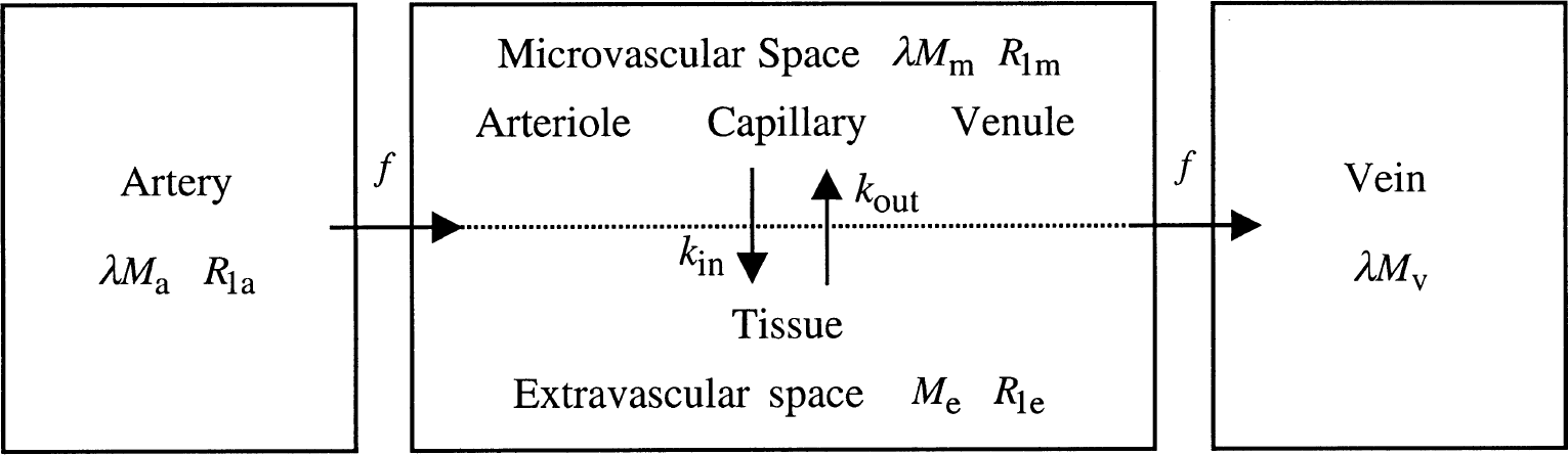
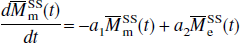
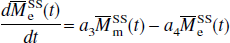
Schematic two-compartment perfusion model for parenchyma using water exchange rates k_in and k_out to describe restricted water exchange. The small microvascular compartment (m) reflects water in arterioles, capillaries, and venules with a total volume CBV. The large extravascular compartment (e) reflects tissue water. Units for the magnetizations reflect the character of the compartment (per milliliter blood and per gram brain for M_m and M_e, respectively) and are converted through the brain/blood partition coefficient X.

$\begin{array}{lll}\frac{d[\lambda M_{\mathrm{m}}(t)]}{dt}\hfill & =\hfill & -R_{1\hspace{0.17em}\mathrm{m}}[\lambda M_{\mathrm{m}}(t)-\lambda M_{\mathrm{m}0}]-k_{\text{in}}\lambda M_{\mathrm{m}}(t)\hfill \\ \hfill & \hfill & +k_{\text{out}}{M}_{\mathrm{e}}(t)+f[M_{\mathrm{a}}(t)-M_{\mathrm{v}}(t)]\hfill \end{array}$

(1a)

$\begin{array}{lll}\frac{d{M}_{\mathrm{e}}(t)}{dt}\hfill & =\hfill & -R_{1\hspace{0.17em}\mathrm{e}}[M_{\mathrm{e}}(t)-M_{\mathrm{e}0}]+k_{\text{in}}\lambda M_{\mathrm{m}}(t)\hfill \\ \hfill & \hfill & -k_{\text{out}}{M}_{\mathrm{e}}(t)\hfill \end{array}$

(1b)

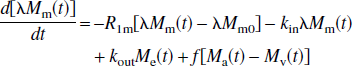
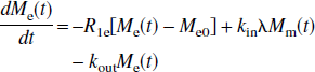
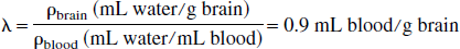
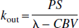
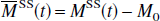
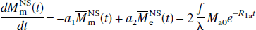
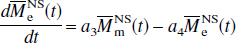
where M_a and M_v are the longitudinal magnetizations of water in incoming arterial blood and leaving venous blood, respectively. This water delivery to and export from the microvasculature is not a part of the two-compartment parenchymal model and indicates the magnetization difference for water in pure blood determined by flow (f) in case of no exchange. The constants k_in and k_out are the effective exchange rates of water from the microvascular space to extravascular space (inward) and vice versa (outbound), respectively. As explained later, these effective rates should not be interchanged with the exact capillary exchange rates and should not be confused with the magnetization transfer rates between tissue water and macromolecules discussed in the single-compartment model by Silva et al. (1997a). This latter effect is included in the effective tissue relaxation rate R_1e. As usual, λ is the brain/blood partition coefficient for water (Herscovich and Raichle, 1985), which is the ratio of the water densities in brain and blood:

$\lambda =\frac{{\rho }_{\text{brain}}(\text{mL}\hspace{0.17em}\text{water}/\mathrm{g}\hspace{0.17em}\text{brain})}{{\rho }_{\text{blood}}(\text{mL}\hspace{0.17em}\text{water}/\text{mL}\hspace{0.17em}\text{blood})}=0.9\hspace{0.17em}\text{mL}\hspace{0.17em}\text{blood}/\mathrm{g}\hspace{0.17em}\text{brain}$

(2)

When the system is in equilibrium, the magnetization values obey the relations:

$k_{\text{in}}\lambda M_{\mathrm{m}0}=k_{\text{out}}{M}_{\mathrm{e}0}$

(3a)

$M_{\mathrm{a}0}=M_{\mathrm{v}0}$

(3b)

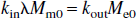
It is obvious that the two exchange rates, k_in and k_out, are not equal because of the different volumes, λM_m0 and M_e0. Assuming that arterial water, venous water, and parenchymal water have the same unitary equilibrium magnetization, M₀, it can then be derived that:

$M_0=\lambda M_{\mathrm{a}0}=\lambda M_{\mathrm{v}0}=\lambda M_{\mathrm{m}0}+M_{\mathrm{e}0}=\lambda M_{\mathrm{m}0}(1+k_{\text{in}}/k_{\text{out}})$

(4)

where (1 + k_in/k_out) is the transformation factor between the longitudinal magnetizations of arterial (or venous) blood water and microvascular blood water, and the ratio k_in/k_out = M_e0/λM_m0 signifies the relative population of water spins in the extravascular and microvascular compartments.

Exchange rates of water. The new perfusion model used in this article consists of two compartments, microvessels and surrounding tissue, with the exchange taking place in the posterior arterioles and the capillaries. Consequently, the differential equations (Eqs. 1a and 1b) for the magnetization not only have R₁ and flow terms, but also have a contribution reflecting the exchange rates of water between the microvascular space and the extravascular space, k_in and k_out. Although the exchange rates and the flow in principle can be obtained by fitting the FAIR signal intensity differences as a function of inversion recovery time (TI), this procedure is inaccurate because of the practical limitations of poor signal-to-noise ratio for the FAIR signal-intensity differences (a few percent of the total signal intensity) and the uncertainty of multiparameter fitting. As demonstrated by Schwarzbauer et al. (1997), however, the two exchange rates for water can be estimated using the appropriate CBV and the permeability-surface area product for water. These relationships are:

$k_{\text{in}}=\frac{PS}{CBV}$

(5a)

$k_{\text{out}}=\frac{PS}{\lambda -CBV}$

(5b)

Using these equations, the absolute fractional populations of water spins in the microvascular and extravascular compartments, p_m and p_e, can be obtained:

$p_{\mathrm{m}}=k_{\text{out}}/(k_{\text{in}}+k_{\text{out}})=CBV/\lambda$

(6a)

$p_{\mathrm{e}}=k_{\text{in}}/(k_{\text{in}}+k_{\text{out}})=(\lambda -CBV)/\lambda$

(6b)

in which p_m + p_e = 1. To determine the rate constants, k_in and k_out, the authors searched the literature for capillary PS and CBV. Blood volumes and permeability-surface products have been obtained for humans and animals by various techniques (Eichling et al., 1974; Larson et al., 1987; Grubb et al., 1974; Raichle et al., 1983; van Zijl et al., 1998; Paulson et al., 1977; Herscovich et al., 1987; Berridge et al., 1991; Sakai et al., 1985; Perlmutter et al., 1987; Leenders et al., 1990; Muizelaar et al., 1997). Data from some mammal studies are shown in Table 1, where rat data have been excluded because of the substantial difference with other mammals. These numbers show reasonable agreement between mammals; and, as only limited cat data and limited separated gray and white matter data are available, the authors used the average whole-brain human results from these data. This is not unrealistic in view of the similar CBV for cats and humans. Assuming 3:1 and 4:3 gray-to-white matter ratios for animals and humans, respectively, the authors found PS = 137 mL 100 g⁻¹ min⁻¹ and CBV = 4.5 mL/100 g, leading to k_in = 0.51 sec⁻¹, k_out = 0.027 sec⁻¹. It is important to point out that the CBV value used is for the complete microvasculature and not just the capillaries. The validity of this will be discussed after the final solutions for the differential equations including the effect of transit time delays have been derived and the results for exchange rates based on capillary and microvascular CBV are compared.

TABLE 1.

Capillary permeability-surface products for water and cerebral blood volumes for several mammals

Species	Anesthesia	Tissue	PS (mL 100 g−1 min−1)	CBV* (mL/100 g)	Reference
Monkey	Phencyclidine	Hemisphere	138		(Eichling et al., 1974)
Monkey	Phencyclidine	Hemisphere	173		(Larson et al., 1987)
Monkey	Phencyclidine	Hemisphere		3.5	(Grubb et al., 1974)
Baboon	70% NO2	Hemisphere	104		(Raichle et al., 1983)
Cat	Halothane	GMWM		5.22.2	(van Zijl et al., 1998)
Human	Awake	Hemisphere	169		(Paulson et al., 1977)
Human	Awake	Hemisphere	104		(Herscovich et al., 1987)
		Cortex	127
		WM	80
Human	Awake	Hemisphere	133		(Berridge et al., 1991)
Human	Awake	Hemisphere		4.8	(Sakai et al., 1985)
Human	Awake	Whole Brain		4.9	(Perlmutter et al., 1987)
Human	Awake	GMWM		5.02.5	(Leenders et al., 1990)
Human	Awake	Hemisphere		5.3	(Muizelaar et al., 1997)

*

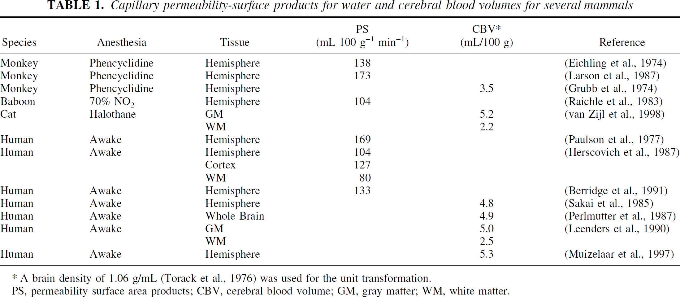
A brain density of 1.06 g/mL (Torack et al., 1976) was used for the unit transformation.

PS, permeability surface area products; CBV, cerebral blood volume; GM, gray matter; WM, white matter.

Working equations for slice-selective and nonselective inversion. Assuming that the tagging volume is completely replenished with fresh blood before each inversion and using Eq. 4, the longitudinal magnetizations of arterial and venous blood water for the slice-selective (SS) and nonselective (NS) measurements can be written as the following:

$M_{\mathrm{a}}^{\text{SS}}(t)=M_{\mathrm{a}0}=(1+k_{\text{in}}/k_{\text{out}})M_{\mathrm{m}0}$

(7a)

$M_{\mathrm{v}}^{\text{SS}}(t)=(1+k_{\text{in}}/k_{\text{out}})M_{\mathrm{m}}^{\text{SS}}(t)$

(7b)

and

$\begin{array}{lll}{M}_{\mathrm{a}}^{\text{NS}}(t)\hfill & =\hfill & M_{\mathrm{a}0}(1-2e^{-R_{1a}t})\hfill \\ \hfill & =\hfill & (1+k_{\text{in}}/k_{\text{out}})M_{\mathrm{m}0}(1-2e^{-R_{1a}t})\hfill \end{array}$

(8a)

$M_{\mathrm{v}}^{\text{NS}}(t)=(1+k_{\text{in}}/k_{\text{out}})M_{\mathrm{m}}^{\text{NS}}(t)$

(8b)

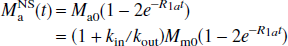
where R_1a is the spin-lattice relaxation rate for the arterial blood water. Unlike the single-compartment tissue model, in which the longitudinal magnetization of the leaving venous water is assumed to be proportional to the parenchymal magnetization, the two-compartment model assumes that the venous longitudinal magnetization correlates only with the microvascular magnetization, but not directly with the extravascular tissue magnetization. Therefore, for the SS inversion, Eqs. 1a and 1b can be rewritten as:

$\frac{d{\overline{M}}_{\mathrm{m}}^{\text{SS}}(t)}{dt}=-a_1{\overline{M}}_{\mathrm{m}}^{\text{SS}}(t)+a_2{\overline{M}}_{\mathrm{e}}^{\text{SS}}(t)$

(9a)

$\frac{d{\overline{M}}_{\mathrm{e}}^{\text{SS}}(t)}{dt}=a_3{\overline{M}}_{\mathrm{m}}^{\text{SS}}(t)-a_4{\overline{M}}_{\mathrm{e}}^{\text{SS}}(t)$

(9b)

in which, for convenience, the authors introduced a reduced longitudinal magnetization and several constants:

${\overline{M}}^{\text{SS}}(t)=M^{\text{SS}}(t)-M_0$

(10)

$a_1=R_{1\mathrm{m}}+k_{\text{in}}+(1+k_{\text{in}}/k_{\text{out}})f/\lambda$

(11a)

$a_2=k_{\text{out}}/\lambda$

(11b)

$a_3=k_{\text{in}}\lambda$

(11c)

$a_4=R_{1\mathrm{e}}+k_{\text{out}}$

(11d)

Similarly, for the NS inversion, Eqs. 1a and 1b can be represented in the following form:

$\frac{d{\overline{M}}_{\mathrm{m}}^{\text{NS}}(t)}{dt}=-a_1{\overline{M}}_{\mathrm{m}}^{\text{NS}}(t)+a_2{\overline{M}}_{\mathrm{e}}^{\text{NS}}(t)-2\frac{f}{\lambda }{M}_{\mathrm{a}0}{e}^{-R_{1\mathrm{a}}t}$

(12a)

$\frac{d{\overline{M}}_{\mathrm{e}}^{\text{NS}}(t)}{dt}=a_3{\overline{M}}_{\mathrm{m}}^{\text{NS}}(t)-a_4{\overline{M}}_{\mathrm{e}}^{\text{NS}}(t)$

(12b)

Solutions without transit times. Equations 9a, 9b, 12a, and 12b can be solved analytically (see Appendix I). The total longitudinal magnetization for the parenchyma can be calculated from the sum of the microvascular and tissue components (see Appendix I), and the FAIR signal intensity is found by subtracting the NS solution from the SS solution. The authors excluded the voxels located at or near the large vessels, such as the draining veins, whose signals may be dephased by extra crusher gradients (Ye et al., 1997). The FAIR signal-intensity differences for microvasculature, tissue, and parenchyma as a function of TI (inversion recovery time) can be derived as:

$\begin{array}{lll}\lambda \Delta M_{\mathrm{m}}(TI)\hfill & =\hfill & \lambda [{\overline{M}}_{\mathrm{m}}^{\text{SS}}(TI)-{\overline{M}}_{\mathrm{m}}^{\text{NS}}(TI)]=\frac{2M_{0}f/\lambda }{R_{1\mathrm{a}}^{\hspace{0.17em}\hspace{0.17em}\hspace{0.17em}\hspace{0.17em}\hspace{0.17em}2}-A{R}_{1\mathrm{a}}+B}\hfill \\ \hfill & \hfill & \left[(k_{\text{out}}+R_{1\mathrm{e}}-R_{1\mathrm{a}})e^{-R_{1\mathrm{a}}TI}-\frac{(\beta -R_{1\mathrm{a}})(\alpha -k_{\text{out}}-R_{1\mathrm{e}})}{\alpha -\beta }{e}^{-\alpha \hspace{0.17em}TI}+\frac{(\alpha -R_{1\mathrm{a}})(\beta -k_{\text{out}}-R_{1\mathrm{e}})}{\alpha -\beta }{e}^{-\beta \hspace{0.17em}TI}\right]\hfill \end{array}$

(13a)

$\Delta M_{\mathrm{e}}(TI)={\overline{M}}_{\mathrm{e}}^{\text{SS}}(TI)-{\overline{M}}_{\mathrm{e}}^{\text{NS}}(TI)=\frac{2M_{0}f/\lambda }{R_{1\mathrm{a}}^{\hspace{0.17em}\hspace{0.17em}\hspace{0.17em}\hspace{0.17em}\hspace{0.17em}2}-{\text{AR}}_{\text{1a}}+B}{k}_{\text{in}}\left[e^{-R_{1\mathrm{a}}TI}+\frac{\beta -R_{1\mathrm{a}}}{\alpha -\beta }{e}^{-\alpha \hspace{0.17em}TI}-\frac{\alpha -R_{1\mathrm{a}}}{\alpha -\beta }{e}^{-\beta \hspace{0.17em}TI}\right]$

(13b)

$\begin{array}{lll}\Delta M(TI)\hfill & =\hfill & \lambda \Delta M_{\mathrm{m}}(TI)+\Delta M_{\mathrm{e}}(TI)=\frac{2M_{0}f/\lambda }{R_{1\mathrm{a}}^{\hspace{0.17em}\hspace{0.17em}\hspace{0.17em}\hspace{0.17em}2}-A{R}_{1\mathrm{a}}+B}\hfill \\ \hfill & \hfill & [(k_{\text{in}}+k_{\text{out}}+R_{1\mathrm{e}}-R_{1\mathrm{a}})e^{-R_{1\mathrm{a}}TI}-\frac{(\beta -R_{1\mathrm{a}})(\alpha -k_{\text{in}}-k_{\text{out}}-R_{1\mathrm{e}})}{\alpha -\beta }{e}^{-\alpha \hspace{0.17em}TI}\hfill \\ \hfill & \hfill & +\frac{(\alpha -R_{1\mathrm{a}})(\beta -k_{\text{in}}-k_{\text{out}}-R_{1\mathrm{e}})}{\alpha -\beta }{e}^{-\beta \hspace{0.17em}TI}]\hfill \end{array}$

(13c)

respectively, in which

$A=a_1+a_4$

(14a)

$B=a_1{a}_4-a_2{a}_3$

(14b)

$\alpha =\frac{1}{2}\left[(a_1+a_4)+\sqrt{{(a_1-a_4)}^2+4a_2{a}_3}\right]$

(15a)

$\beta =\frac{1}{2}\left[(a_1+a_4)-\sqrt{{(a_1-a_4)}^2+4a_2{a}_3}\right]$

(15b)

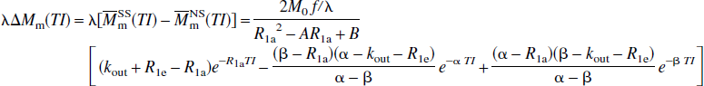
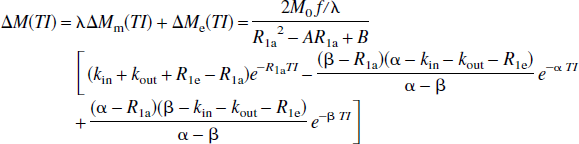
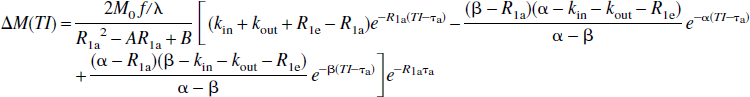
Thus, these FAIR signal-intensity differences as a function of TI are triexponentials with relaxation rates α, β, and R_1a. It is important to notice that these signal-intensity differences at a certain TI are predelay-independent (Zhou and van Zijl, 1999a,1999b), even though the microvascular, tissue, and parenchymal (total) signal intensities for the SS and NS scans depend on the predelay (see Appendix I), in which the predelay τ is defined as the time interval from the 90† slice-selective pulse to the inversion pulse of the next scan. In addition, as expected, the individual FAIR signal-intensity difference for the extravascular compartment is 0 if k_in = 0.

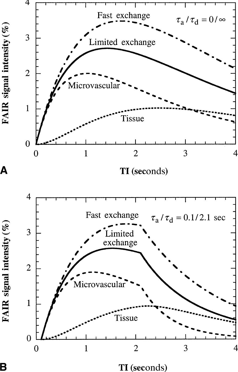
In the conventional model of fast exchange (k_in, k_out ≫ R_1m, R_1e), the relaxation rates α and β can be simplified (see Appendix II), and the e^−αTI terms become negligible compared with the e^−βTI terms due to relatively fast decaying rate (α >> β) and relatively small coefficients. Consequently, Eq. 13c is reduced to the familiar result (Kwong et al., 1995; Calamante et al., 1996; Zhou and van Zijl, 1999a):

$\Delta M(TI)=\frac{2M_{0}f/\lambda }{R_{1\hspace{0.17em}\text{app}}-R_{1\mathrm{a}}}(e^{-R_{1\mathrm{a}}TI}-e^{-R_{1\hspace{0.17em}\text{app}}TI})$

(16)

in which R_1app = R₁ + f/λ, and R₁ = p_m R_1m + p_eR_1e is the weighted average of the spin-lattice relaxation rates of microvascular and tissue water.

Solutions with transit times. In general, the volume of the tagging bolus is not infinite, especially when using surface coils, which have a limited excitation range. Assume that τ_a and τ_d are the transit times for the leading edge and trailing edge of the tagging bolus to reach the capillary exchange site in the imaging slice, respectively. In the presence of finite transit times, as explained previously (Zhou and van Zijl, 1999b), both the SS and NS scans become a mixed NS/SS relaxation process, namely an NS relaxation process followed by an SS process. There are separate equations for the FAIR signal-intensity differences for different time periods during TI, namely for TI ≤ τ_a, τ_a < TI ≤ τ_d, and TI > τ_d. For the cat surface coil experiments, the authors have τ_a ≈ 0.1 second and τ_d ≈ 2.1 seconds (Zhou et al., 1998; Zhou and van Zijl, 1999a, b ) at normal flow, and the equation for the total FAIR signal-intensity difference of interest (TI ≈ T₁ = 1.6 seconds for gray matter) is the one for the period between τ_a and τ_d. This can be derived as:

$\begin{array}{lll}\Delta M(TI)\hfill & =\hfill & \frac{2M_{0}f/\lambda }{R_{1\mathrm{a}}^{\hspace{0.17em}\hspace{0.17em}\hspace{0.17em}\hspace{0.17em}\hspace{0.17em}2}-A{R}_{1\mathrm{a}}+B}[(k_{\text{in}}+k_{\text{out}}+R_{1\mathrm{e}}-R_{1\mathrm{a}})e^{-R_{1\mathrm{a}}(TI-{\tau }_{\mathrm{a}})}-\frac{(\beta -R_{1\mathrm{a}})(\alpha -k_{\text{in}}-k_{\text{out}}-R_{1\mathrm{e}})}{\alpha -\beta }{e}^{-\alpha (TI-{\tau }_{\mathrm{a}})}\hfill \\ \hfill & \hfill & +\frac{(\alpha -R_{1\mathrm{a}})(\beta -k_{\text{in}}-k_{\text{out}}-R_{1\mathrm{e}})}{\alpha -\beta }{e}^{-\beta (TI-{\tau }_{\mathrm{a}})}]e^{-R_{1\mathrm{a}}{\tau }_{\mathrm{a}}}\hfill \end{array}$

(17)

which, for the conventional model of fast exchange, can be simplified as:

$\Delta M(TI)=\frac{2M_{0}f/\lambda }{R_{1\hspace{0.17em}\text{app}}-R_{1\hspace{0.17em}\mathrm{a}}}[e^{-R_{1\mathrm{a}}(TI-{\tau }_{\mathrm{a}})}-e^{-R_{1\hspace{0.17em}\text{app}}(TI-{\tau }_{\mathrm{a}})}]e^{-R_{1\hspace{0.17em}\mathrm{a}}{\tau }_{\mathrm{a}}}$

(18)

In the case of finite transit times, the FAIR signal-intensity difference at a fixed TI remains predelay-independent, but depends on the transit times of the tagging bolus (τ_a and τ_d) and the inward and outbound exchange rates of water (k_in and k_out).

MATERIALS AND METHODS

Animal preparation

Animal care throughout the experimental procedures was in accordance with institutional guidelines. Six mixed-breed male or female cats weighing 2.5 to 3.5 kg were anesthetized with pentobarbital sodium (40 mg/kg, intraperitoneally (IP), followed by 6 mg/kg/h, intravenous (IV) infusion). Catheters were placed into the femoral artery and vein bilaterally to monitor mean arterial blood pressure (MABP) and to collect arterial blood gases, and to administer fluids and drugs, respectively. Cerebral venous blood samples were collected through a small outside diameter catheter inserted into the superior sagittal sinus (data were not used in current article). Animals received 8 mL/kg/h lactated Ringer solution IV during the surgical preparation and 4 mL/kg/h thereafter throughout the experimental protocol. Pancuronium bromide (0.1 mg/kg, IV) was administered for muscle paralysis during electrocauterization and the MRI measurements. Animals were secured in a frame, and head and surface coil were well fixed to avoid motion. Core temperature was maintained with a water-jacketed warming blanket. Body temperature was monitored during the measurements. Animals were ventilated (Harvard Instruments Animal Ventilator, Boston, MA, U.S.A.) using endotracheal intubation. Supplemental oxygen was administered to maintain the arterial partial pressure of oxygen (PaO₂) at greater than 100 mm Hg. To achieve a normocapnic state, ventilatory volume and rate were adjusted to bring PaCO₂ into the 30 to 34 mm Hg range. Hypercapnia was induced by blending CO₂ into the animals' breathing mixture. Hypocapnia was induced by increasing tidal volume, and consequently, minute ventilation. At each level the animals were allowed to stabilize at the new physiologic steady state for 10 to 15 minutes before collecting arterial and cerebral venous blood gas samples for measurement. Magnetic resonance imagining scanning began after sample collection. Cerebral blood flow for comparison was measured by radiolabeled microsphere injection after MRI measurements were obtained. At this time a second pair of arterial and cerebral venous blood samples were collected to ensure that respiratory gases were stable throughout the MRI sampling period. Blood gases and pH were analyzed with a 248 pH/Blood Gas Analyzer (Chiron Diagnostics, Essex, U.K.). Whole blood total hemoglobin content, hemoglobin saturation, and oxygen content were determined with an OSM3 Hemoximeter (Radiometer, Copenhagen, Denmark), using the calculation mode specific for cat hemoglobin. In each animal, 3 to 5 different Paco₂ levels were achieved, each lasting 35 to 40 minutes. After each experiment, the anesthetized cats were killed by IV injection of 6 mL saturated KCl.

Magnetic resonance imaging experiments

Experiments were performed on a horizontal bore 4.7 T GE CSI animal imager (40 cm bore) equipped with shielded gradients of up to 19 G/cm. A surface coil (4-cm inner diameter) was used for radiofrequency (RF) transmission and reception. The FAIRER pulse sequence (Zhou et al., 1998) was used to remove the destructive effects of radiation damping, which may otherwise interfere with the inversion recovery course, the spin echo signal, and the initial magnetization. Adiabatic hyperbolic secant (sech) RF pulses were used for spin inversion. To check whether these sech pulses achieve good inversion behavior for the brain and its feeding vessels at sufficient distance from the coil, the authors performed an experiment in which imaging profiles perpendicular to the coil were acquired. This was done for a range of up to 4 cm from the top of the brain by increasing the power of the RF pulses for detection (and keeping the sech power constant). In all cases over this distance, these profiles could be nulled because of proper inversion. Four-shot echo-planar imaging (EPI) was used with echo time (TE) = 45 milliseconds. The b value for the crusher around the refocusing pulse was 19 sec/cm², to remove only the signal contributions from large vessels. The imaging slice offset was set in the axial plane at 8 mm from the top of brain (4 cats) or in the coronal plane at 15 mm from the occipital pole (2 cats). The imaging matrix was 64 × 64, field of view was 64 × 64 mm², and the imaging slice thickness was 2 mm. The SS inversion slab was centered at the same position as the imaging slice, and its thickness was 6 mm. Seven TI values (0.2, 0.6, 1.25, 1.6, 2.0, 2.8, and 3.4 seconds, 2 cats) with 4 images at every TI or 14 TI values (0.1, 0.2, 0.4, 0.6, 0.8, 1.0, 1.2, 1.4, 1.6, 1.8, 2.0, 2.3, 3.0, and 4.0 seconds, 4 cats) with 2 images at every TI were acquired. The predelay of 2 seconds was used and all scans were preceded by 2 dummy scans.

Data were processed using the IDL software system (Research Systems, Boulder, CO, U.S.A.). The spin-lattice relaxation rates for the two scans, R₁^SSand R₁^NS, were calculated using a three-parameter or monoexponential fit on a pixel-by-pixel basis, and M₀ was obtained simultaneously from the average of the intercepts at long TI for the two fits. Because the SS and NS scans are essentially multiexponential spin-lattice relaxation processes, although not experimentally distinct from monoexponential, the monoexponentially fitted relaxation rates should be regarded as the effective relaxation rates. The fitted FAIR signal-intensity differences at TI = 1.2 (or 1.25) and 1.6 seconds were obtained by subtracting the fitted SS and NS curves and used to calculate the flows. Instead of the experimental signal intensities, the fitted signal intensities through all points were used here to calculate the flows in order to increase the accuracy and precision of the data points (Zhou et al., 1998; Zhou and van Zijl, 1999a). The flow values were averaged over four regions of interest (ROIs) taken in gray matter close to brain surface and were compared with the microsphere CBF values taken from similar cortical gray matter regions cut from the brain. The spatial reference for the cutting was based on the MRI localizer images taken before the flow imaging. The sample for the microsphere determination of blood flow was collected on the dorsal aspect of the brain surface and included tissue from both hemispheres, so it represents an average gray matter value and the two measurements should reflect blood flow in identical regions of interest. For the different PaCO₂ levels of each animal and for the uncorrected and corrected CBF maps at the different TIs of each PaCO₂ level, the same ROIs are chosen by using the T₁ map as a reference.

For the fast exchange approach, the flows quantified by signal-intensity differences were calculated based on Eq. 18, as described previously (Kim, 1995; Kwong et al., 1995), and the apparent relaxation rate of the perfused tissue R_1app was approximated as being equal to the fitted R₁^SS. For restricted exchange, quantification of flow is also possible by using the fitted R₁^SS for the relaxation rate of tissue water R_1e. Using R_1m and R_1a from Results, k_in and k_out from Theory, and the transit time (τ_a) for the arriving bolus as above, the only remaining unknown is the flow. However, extracting the flow (f) directly from the observed signal intensity difference is somewhat cumbersome because of the fact that the flow occurs in several parts of Eq. 17, complicating the rewriting of flow in terms of the only observable, the signal intensity change. To overcome this difficulty, one can use a regressive procedure, such as changing the flow value until the difference between the calculated and measured signal intensity differences is minimal. An alternative procedure is to start with the flow calculated from the fast exchange case, substitute it for all positions in Eq. 17 except for the numerator of the first factor, namely the first term with f/λ, and calculate a new flow. This procedure, which was used here, can be iterated until there is no more change in the calculated flow. It was shown that a larger iterative number may be required for higher flows, but only up to 5 iterations suffice for approaching the true flow of up to 200 mL 100 g⁻¹ min⁻¹ within 0.1%.

Cerebral blood flow measurements using microspheres

Regional CBF was measured with radiolabeled microspheres using the reference withdrawal method (Marcus et al., 1976). Five radioactive isotopes (¹¹⁴In, ¹¹³Sn, ¹⁰³Ru, ⁹⁵Nb, and ⁴⁶Sc, 16 ± 0.5 μm diameter; Du Pont-NEN Products, Boston, MA, U.S.A.) were injected in random sequence in each animal. Approximately 2.5 × 10⁶ microspheres were injected into the left atrium over a 20-second period, followed by 10 mL saline flush. The reference blood sample was withdrawn from the aorta at 1.94 mL/min beginning 30 seconds before the injection and continuing for 90 seconds after the saline flush. Injection of microspheres and withdrawal of reference blood were performed using catheters of 2 m in length. Dead space volume was measured to ensure adequate flush solution after microsphere injection and adequate withdrawal volume for the reference blood samples. After the MRI and microsphere measurements were finished, the brain was removed and placed in 10% formalin for 1 to 2 days before sectioning. After sectioning, brain tissue and withdrawn blood samples were analyzed in an autogamma scintillation spectrometer (5000 Series; Packard Instrument, Downers, Grove, IL, U.S.A.). Blood flow was calculated from CBF = CPM_c/CPM_r. RBF, where CPM_c is counts per minute per 100 g cerebral tissue, CPM_r is counts per minute in the reference sample, and RBF the withdrawal rate of the reference blood sample (mL/min).

RESULTS

Simulations

FAIR signal-difference results without transit times. To obtain an intuitive picture of the magnitude of the FAIR signal-intensity changes originating from the microvasculature and the tissue, the authors calculated these effects (Fig. 2A, Table 2) for several flows using the exchange rates determined in the previous section. The other parameters used for these calculations were R_1a = 0.53 sec⁻¹ or T_1a =1.9 seconds (Schwarzbauer et al., 1996), R_1e = 0.63 sec⁻¹ or T_1e = 1.6 seconds (Zhou et al., 1998), and R_1m = 0.55 sec⁻¹ or T_1m = 1.8 seconds. This R_1m was calculated using the linear relationship between the spin-lattice relaxation rate and the deoxygenated hemoglobin fraction as reported by Meyer et al. (1995) and assuming an average deoxygenated hemoglobin fraction of 20% for the microvasculature. As the T₁ -dependence of water on oxygenation is small (Meyer et al., 1995), this is a good approximation. The results in Fig. 2A and Table 2 clearly show that the FAIR signal-intensity differences originating from the microvascular and extravascular compartments are comparable in magnitude, but that the maximum of the microvascular curve is earlier than that of the tissue curve. The restricted exchange of water between the microvascular and extravascular space leads to a nonlinear increase in the total FAIR signal-intensity differences with increasing flows. The authors further see that the maxima of the total FAIR signal intensities are moved to shorter inversion recovery times with increasing flows, whereas this is not the case in the conventional single-compartment model. Finally, the total signal intensity difference is larger in the fast-exchange model, resulting in an underestimation of the flow for the conventional approach.

TABLE 2.

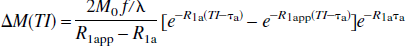
Comparison of the individual and total FAIR signal intensities in gray matter for several flow values

	Microvasculature		Tissue		Total		Old model
f (mL 100 g−1 min−1)	Maximum (%)	TI (sec)	Maximum (%)	TI (sec)	Maximum (%)	TI (sec)	Maximum (%)	TI (sec)
50	0.8	1.21	0.4	2.68	1.1	1.66	1.2	1.74
100	1.4	1.11	0.8	2.57	2.0	1.54	2.3	1.72
150	2.0	1.04	1.0	2.48	2.7	1.44	3.5	1.71
200	2.5	0.97	1.2	2.40	3.3	1.35	4.6	1.70

TI, inversion time.

FIG. 2.

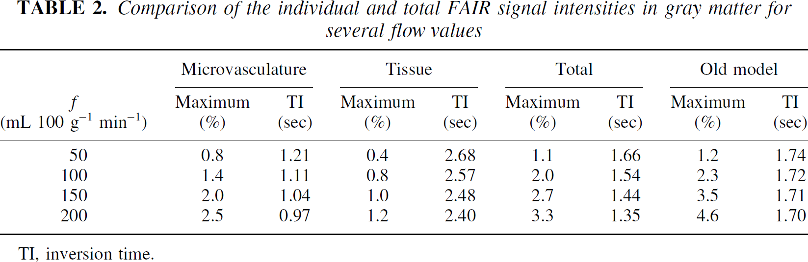
Comparison of the microvascular, tissue, and total (parenchymal) FAIR signal-intensity differences for the case of restricted water exchange with the FAIR signal-intensity difference for the conventional model of fast water exchange. These calculations are (A) in the absence of transit times and (B) in the presence of transit times, τ_a = 0.1 second and τ_d = 2.1 seconds. Other parameters used are k_in = 0.51 sec⁻¹, k_out = 0.027 sec⁻¹, and f = 150 mL 100 g⁻¹ min⁻¹. Compared with fast exchange, the maximum of the FAIR curve for the restricted-exchange model is moved to a short inversion recovery time.

FAIR signal-difference results with transit times. Figure 2B shows a comparison of the microvascular, tissue, and total (parenchymal) FAIR signal-intensity differences for the case of restricted water exchange with that for the conventional model of fast water exchange in the presence of the experimentally estimated transit times T_a = 0.1 second and T_d = 2.1 seconds. Other parameters used were k_in = 0.51 sec⁻¹, k_out = 0.027 sec⁻¹, and / = 150 mL 100 g⁻¹ min⁻¹. Compared with fast exchange, the maximum of the FAIR curve for the restricted-exchange model is moved to a short inversion recovery time. Figure 3 shows the dependence of the total and individual FAIR signal intensities on transit times τ_a (above) and τ_d (below) for the same exchange rates and flow as used in Fig. 2. Under normal flow conditions, the authors estimated τ_a to be less than 0.1 second, so there should be little effect of τ_a on the signal intensity difference at higher flows. The effect of τ_d becomes visible only at measurement times greater than τ_d, which the authors did not reach in their experiment (see below), as verified by looking at the efficiency of nulling profiles for TI = 1.1 second (zero-point of inversion curve) at locations of at least 4 cm from the surface coil.

FIG. 3.

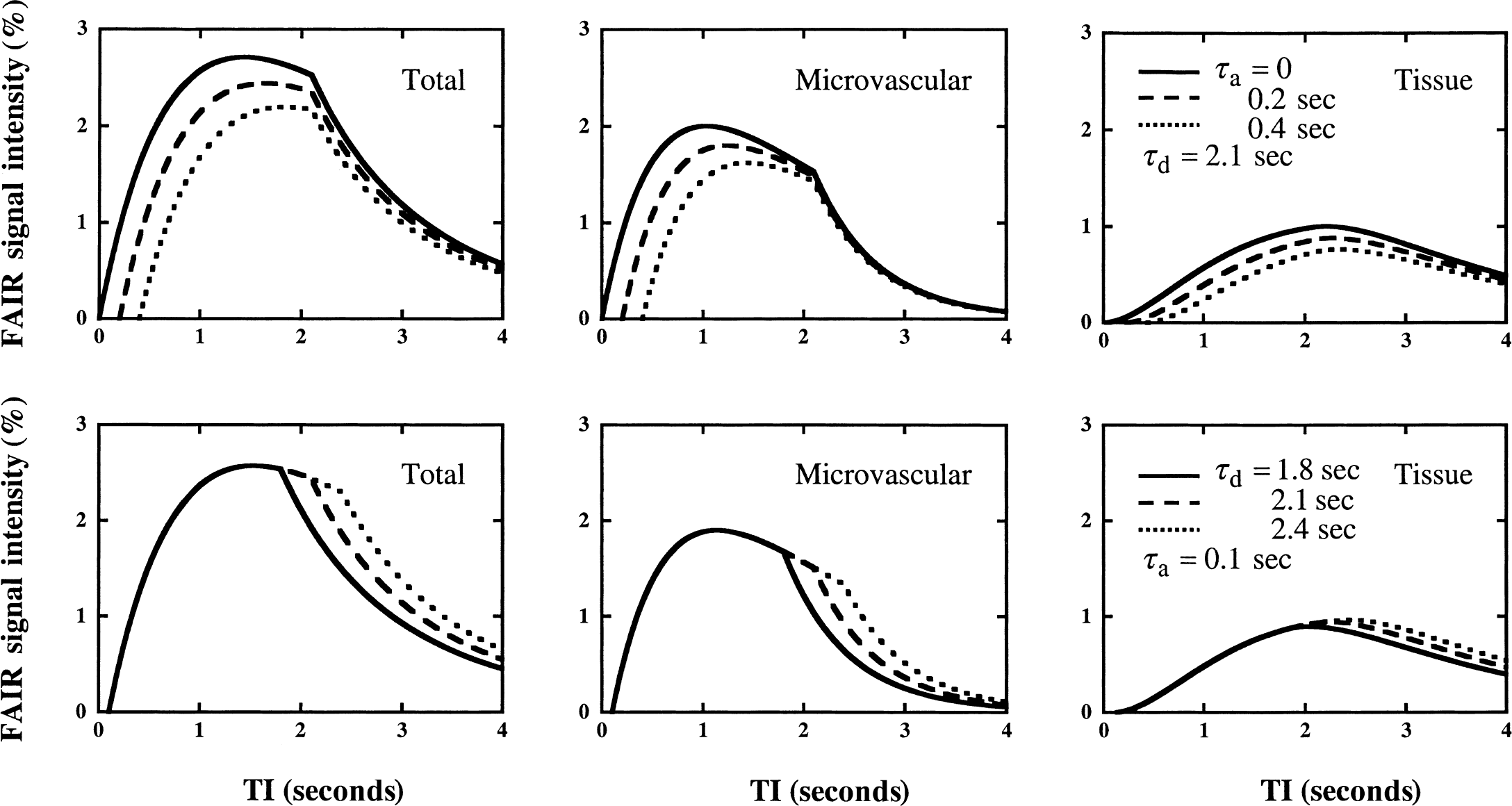
Dependence of the total and individual FAIR signal-difference intensities on transit times τ_a (top) and τ_d (bottom). Other parameters used are k_in = 0.51 sec⁻¹, k_out = 0.027 sec⁻¹, and f = 150 mL 100 g⁻¹ min⁻¹.

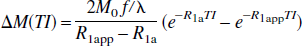
It is important to realize that when restricted exchange is assumed to be fast exchange a significant flow error will appear in the signal-difference approach. This effect at 4.7 T is shown in Fig. 4 (solid line), using the same exchange rates and relaxation rates as in Figs. 2 and 3. In the calculations, the FAIR signal-intensity difference (ΔM) for each true flow (f) was generated by Eq. 17, and the corresponding apparent flow (f_app) was then calculated by Eq. 18. The results show that this error, namely the deviation from the line of identity, increases with increasing flows, because of the reduction in the extraction fraction of water. Interestingly, the theoretical MRI results (solid line) for the two-compartment parenchymal model agree well with the PET curve (dash-dotted line) calculated with the equations f_app = fE = f(1 − e^−PS/f) and PS = 1.50f + 20.6 (Herscovich et al., 1987). This shows the reasonableness of the proposed two-compartment model with the chosen exchange rates based on the total microvascular blood volume instead of the capillary volume.

FIG. 4.

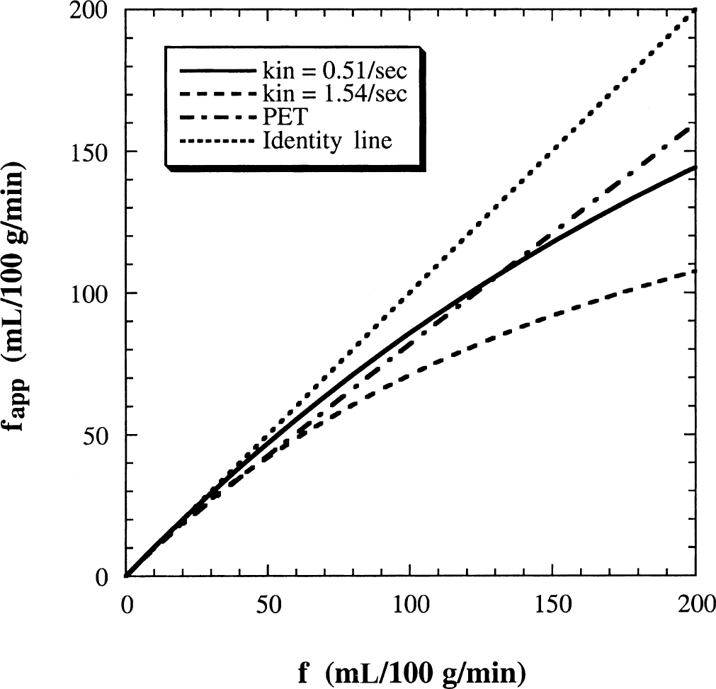
Calculated apparent magnetic resonance imaging flow values obtained with the conventional model from the FAIR signal-intensity difference plotted as a function of the true flows. The FAIR signal intensities were calculated from the two-compartment model using k_in = 0.51 sec⁻¹ and k_out = 0.027 sec⁻¹ (solid line). The restricted exchange of water between the microvascular and tissue compartment leads to a progressive underestimation of calculated flows when using the fast-exchange approach. The apparent positron emission tomography (PET) flow curve (dash-dotted line) calculated with and PS = 1.50f + 20.6 (Herscovich et al., 1987) compares well with the predicted curve based on these exchange rates for the total CBV, but not with the predicted curve (dashed line) for exchange rates (k_in = 1.54 sec⁻¹ and k_out = 0.026 sec⁻¹) based on the use of capillary blood volume.

FAIR signal-difference results using capillary blood volumes. The previous simulations used total microvascular CBV to determine the exchange rates, whereas the actual exchange takes place only in the posterior arterioles and the capillaries. To check how this extraction curve compared with the authors' theory, the authors added the calculated relationship between true and apparent flows based on the k_in and k_out values using capillary CBV (k_in = 1.54 sec⁻¹ and k_out = 0.026 sec⁻¹) to Fig. 4 (dashed line). In doing this, it was assumed that the capillary space contains 33% of the microvascular cerebral blood volume as defined by Sharan et al. (1989; van Zijl et al., 1998). The results in Fig. 4 show that the use of the capillary CBV is not consistent with the PET extraction curve obtained using the same PS values, whereas the use of the total CBV is consistent.

FAIR T₁-difference results. Although rather uncommon, it has sometimes been suggested to use differences of absolute relaxation times instead of signal intensities. For completion, this case also is discussed here. In the presence of finite transit times, the curve for the recovery of longitudinal magnetization as a function of TI is not monoexponential. Consequently, the monoexponentially-fitted spin-lattice relaxation times for the SS and NS measurements depend not only on the individual relaxation rates (R_1m, R_1e, and R_1a) and the flow, but also on the transit times of the tagging bolus, the predelay, and the exchange rates (k_in and k_out). Figure 5 shows the apparent flows quantified from the T₁ difference as a function of the predelay for flows of 50 and 150 mL 100 g⁻¹ min⁻¹ in the experimental cat setup, where τ_a ≈ 0.1 second and τ_d ≈ 2.1 seconds (Zhou et al., 1998; Zhou and van Zijl, 1999a, b ). The calculated apparent flows in the T₁-difference approach are significantly overestimated in both approaches. For fast exchange, the increases are 43% at long predelay and 101% at short predelay for f = 50 mL 100 g⁻¹ min⁻¹ and 41% and 97%, respectively, at f = 150 mL 100 g⁻¹ min⁻¹. These effects, because of the influence of short predelay and finite transit times of the tagging bolus, are somewhat reduced when determining flows using the restricted exchange model, but the flow values are still overestimated by as much as 39% to 95% and 23% to 71% for the low and high flows, respectively. Thus, it is not practical to try to quantify flows directly from the absolute T₁-difference because it is very difficult to take into account the effects arising from short predelays, finite transit times, and limited exchange of water between the microvascular and surrounding tissue compartments.

FIG. 5.

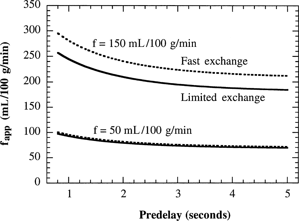
Plot of apparent flows calculated from the FAIR T₁-difference as a function of predelay. Parameters used are k_in = 0.51 sec⁻¹, k_out = 0.027 sec⁻¹, τ_a = 0.1 second, τ_d = 2.1 seconds, TI_max = 4 seconds (longest inversion recovery time (Zhou and van Zijl, 1999a, b )), f = 50, and 150 mL 100 g⁻¹ min⁻¹. The effects of short predelay and finite transit times increase the apparent flows, whereas the effect of limited exchange of water partially compensates for this calculated apparent flow increase.

Experimental results

The cerebral blood flow results for gray matter in six cats during hypocapnia, normocapnia, and hypercapnia are shown in Fig. 6, where the flow values quantified from the FAIR signal differences at 1.6 seconds are compared with those determined by the radiolabeled microsphere technique. Data for both axial (closed circles) and coronal planes (open circles) are given. These data clearly show that flows determined for the single-compartment model (Fig. 6A) are less than those using radioactive microspheres, especially for high flows, so that most of the experimental points in Fig. 6A are located below the line of identity. However, the results for the two-compartment model (Fig. 6B) and the microspheres are comparable, and the experimental points in Fig. 6B are almost equally distributed around the line of identity. To check whether there is influence of reduced τ_d at higher flow rates, Fig. 7 compares the measured CBF numbers of gray matter calculated at short TI (1.2 or 1.25 seconds) and long TI (1.6 seconds) for the 6 cats. It can be seen that the determined CBF variation in this TI range is negligible in the flow range of 15 to 150 mL 100 g⁻¹ min⁻¹ for the experimental setup, showing that the surface coil approach used here is still reliable for the flow range studied.

FIG. 6.

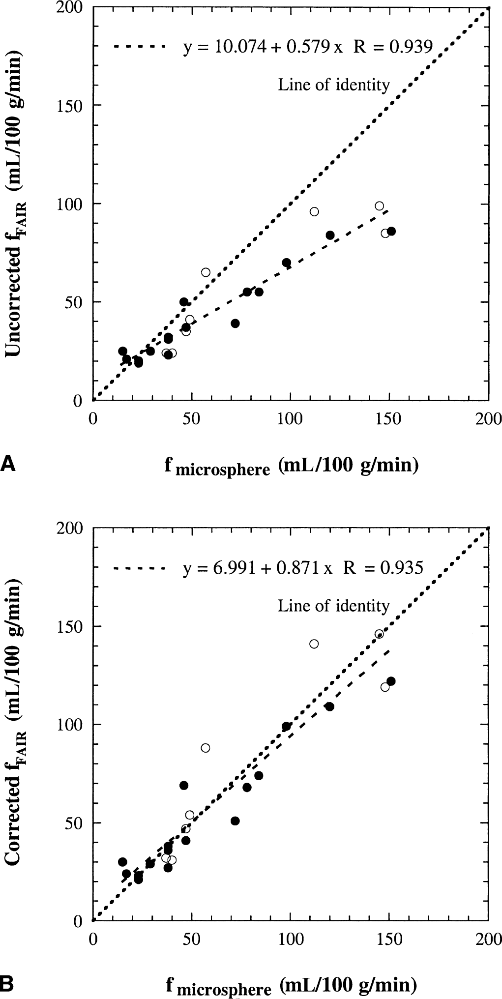
Comparison of flow values measured by the FAIR signal-difference method (filled circles for axial plane and open circles for coronal plane) and by radioactive microspheres for six cats. The FAIR results are for (A) the original single-compartment model and (B) the two-compartment tissue model. The dotted lines are the lines of identity, and the dashed lines represent a linear fit of the results.

FIG. 7.

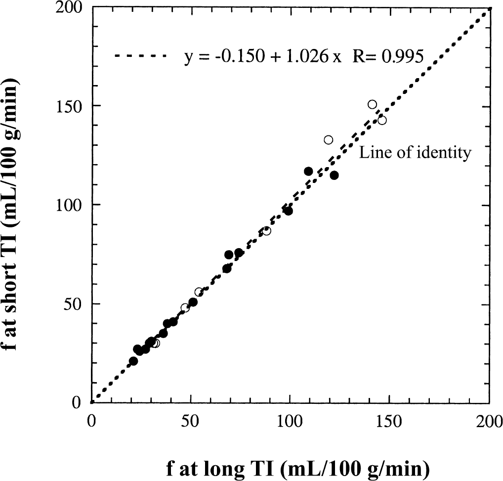
Comparison of the cerebral blood flow values for gray matter quantified from the FAIR signal-intensity differences at short TI (1.2 or 1.25 seconds) and long TI (1.6 seconds) for 6 cats. Filled circles are for axial plane, and open circles are for coronal plane.

DISCUSSION

Theoretical predictions versus experimental results

Assuming that the flow values determined by the radiolabeled microsphere technique are correct, the experimental results in Fig. 6A show that the CBF values measured by FAIR with the original well-mixed compartment model underestimate the actual flow. The deviation increases for higher flow rates, confirming the theoretical predictions in Fig. 4 (solid line). When correcting for finite water exchange between the microvascular compartment and the tissue compartment, there is a good correspondence between the MRI and microsphere data (Fig. 6B). Consequently, it is concluded that it is necessary to correct for restricted exchange of water using the two-compartment perfusion model when measuring cerebral blood flows using arterial spin labeling. This is not unexpected in view of the time scale of the signal-intensity difference experiment (1 to 2 seconds, which depends on the life time of label or the spin-lattice relaxation time of labeled blood water) and the half-life time of water in the microvasculature (including arterioles, capillaries, and venules, ln2/k_in = 1.4 seconds), which are comparable in magnitude. This implies that blood water in the microvascular space and tissue water in the extravascular space do not mix instantaneously, and that a large fraction of the tag will remain in the microvasculature during the time interval of TI < 2 seconds. Thus, in the TI range in which the FAIR signal-intensity differences are measured, the contribution of the small microvascular compartment to the total FAIR signal intensities is actually larger than that of the large tissue compartment, as shown in Figs. 2 and 3, and Table 2. This incomplete mixing of the tagged water spins between the small microvascular compartment and the large tissue compartment corresponds to a reduced extraction fraction of water and loss of label by outflow and results in an underestimation of measured FAIR flows unless a correction for restricted exchange is applied.

The tissue compartment model used in this article is similar to the communicating two-compartment model used in PET by Gambhir et al. (1987), which is not being used extensively in PET, because results are not significantly better than several single-compartment models. With respect to this, it is important to point out that there are several differences between MRI and PET. First, the time scale of the PET labeling experiments is longer than that of the MRI experiments (a few minutes of label accumulation versus seconds). This implies that, for PET, the extravascular contribution to the parenchymal radioactivity is expected to be much larger than the vascular contribution, thereby reducing the importance of exchange delays. Second, a relative population of 1/19 in the 2 compartments has been used in the authors' model, whereas Gambhir et al. (1987) assumed a ratio of 1/4, which seems unrealistic. These differences between the two tissue compartment models render the MRI approach more applicable experimentally.

Field dependence of the exchange effect

The fact that the time scale of the MRI experiments (1 to 2 seconds) is close to the time scale of the water exchange (approximately 1 seconds) between intra- and extravascular space has an interesting consequence, namely that the exchange influence will change as a function of magnetic field strength. The reason being that the MRI time scale changes because longitudinal relaxation rates of water are field dependent and reduce at higher field. Figure 8 shows that the effect of field strength on the apparent flow as calculated by the single-compartment model is significant. These curves were derived by calculating the FAIR signal intensity differences from the two-compartment model for a true flow f, and subsequently determining the apparent flows f_app with the single-compartment model. Results show that for functional MRI experiments, in which flows between 50 and 100 mL 100 g⁻¹ min⁻¹ are normal, it is necessary to start using the two-compartment model at fields above 2 to 3 T.

FIG. 8.

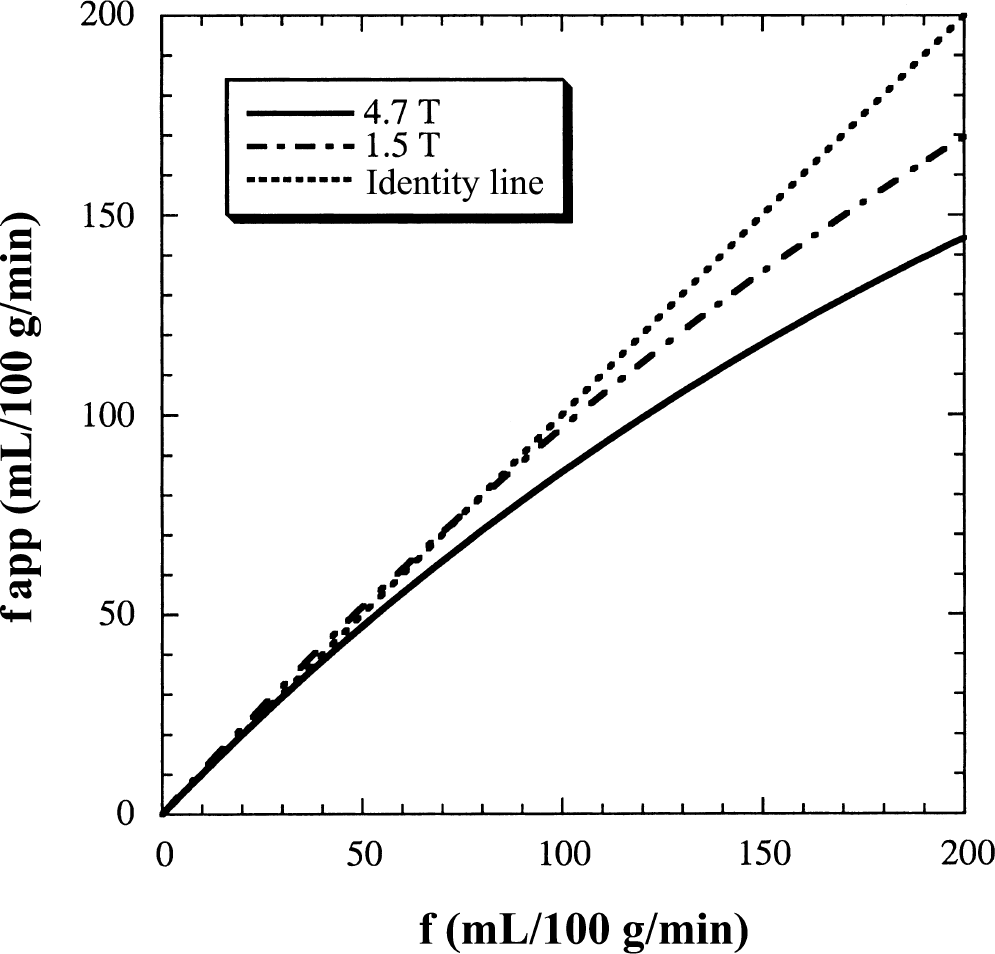
Magnitude of underestimation of flow by the single-compartment approach as a function of field strength. The curves were derived by starting with a true flow, f, implementing it in the two-compartment model and calculating the FAIR signal intensity differences. These were subsequently fitted with the single-compartment model to obtain the apparent flows. Values used for the relaxation rates were T_1a = T_1m = 1.2 seconds and T_1e = 0.9 seconds (Kwong et al., 1995) at 1.5 T, and T_1a = 1.9 seconds, T_1m = 1.8 seconds, and T_1e = 1.6 seconds (see Theory) at 4.7 T.

Even though the restricted exchange of water between the microvascular space and extravascular space reduces the extraction fraction of water, a competing effect introduced by incomplete water extraction, namely the overestimation of the label decay, should be noticed. Because blood has a longer relaxation time than extravascular tissue (T_1m > T_1e) (Calamante et al., 1996; Schwarzbauer et al., 1996), the fact that an increasing amount of labeled water spins remain in the microvascular space would lead to an increase of the apparent flows because of the incorrectly estimated decay, thus partially compensating for the limited exchange effect. An analogous overestimation effect occurs in the single parenchymal model (Kwong et al., 1995; Calamante et al., 1996; Zhou and van Zijl, 1999a). It is important to point out that there are more labeled spins in the microvascular space on the time scale of the signal-intensity-difference approach at lower fields such as 1.5 T, where ΔM is generally calculated at TI = 1 to 1.2 seconds, whereas it is done at TI = 1.6 seconds at 4.7 T. The theoretical calculations in Fig. 8 clearly show that, although the effect is small, it is noticeable at low flow rates, especially at lower fields.

Validity of the exchange rates chosen for water

In the current article, the authors followed Schwarzbauer et al. (1997) and estimated the exchange rates of water using the average permeability-surface area product and cerebral blood volume from large mammals in the literature. These two exchange rates, k_in = 0.51 sec⁻¹ and k_out = 0.027 sec⁻¹, have been used for all restricted exchange calculations. Obviously, the first questions that arise are how accurate are these estimates and how would the small differences in these values influence the measured flows. For example, based on Eqs. 5a and 5b and the fact that CBF and CBV are interdependent through the central volume principle, it could be concluded that the water exchange rates as defined in these equations are flow-dependent. The reason is that S is the product of the circumference (2πr) and length of the capillaries, whereas CBV is the product of the length and cross section area (πr²). However, upon further inspection, this is not the case for k_in. This was checked using the PS/CBF data reported in humans by Herscovitch et al. (1987), who reported the flow dependence of PS. The correspondence between PS and CBV can then be calculated by using derived and measured relationships between CBF and CBV, such as CBV = 0.5f^0.5 (van Zijl et al., 1998) or CBV = 0.8f^0.38 (Grubb et al., 1974). When the resulting PS/CBV data were fitted by a linear equation, the authors obtained PS = 0.48CBV (R = 0.82) and PS = 0.50CBV (R = 0.76) for these two equations, respectively, corresponding to k_in values of 0.48 sec⁻¹ and 0.50 sec⁻¹. Thus, within the experimental data spread of these measurements, the authors' assumption that PS is proportional to CBV is valid and k_in is constant.

Another point that needs to be addressed is the fact that water exchange occurs mainly between capillaries and tissue. This means that the two-compartment perfusion model is also an approximation and that a much more complex four-compartment model (arterioles, capillaries, venules, and tissue) may be necessary to more accurately describe the effect of exchange in arterial spin tagging. However, such a four-compartment model will induce more parameters and is beyond the goal of the current study. Therefore, the authors used a simplified approach in which the exchange rates of water are related to published capillary permeability-surface area product of water and the total microvascular cerebral blood volume. This seems contradictory and needs further explanation. To better understand the approach, it is important to realize that the reported capillary PS measurements (Eichling et al., 1974; Go et al., 1981; Raichle et al., 1983; Herscovich et al., 1987; Berridge et al., 1991; Schwarzbauer et al., 1997; Larson et al., 1987; Paulson et al., 1977; Reid et al., 1983) actually did not separate capillaries from arterioles and venules, and that the measured PS values were the average numbers over all microvessels. Consequently, combining these empirical PS values with the total microvascular blood volume values (or the total CBV as measured previously by PET) for the purpose of estimating the water exchange rates should be a good approximation. These calculated rates should be viewed as the effective exchange rates in the two-compartment model, even though they are not the true exchange rates between capillaries and tissue. To verify whether such an approach does not introduce large errors, the authors calculated the relationship between true and apparent flows based on k_in and k_out values derived using total CBV (k_in = 0.51 sec⁻¹ and k_out = 0.027 sec⁻¹) as well as capillary CBV (k_in = 1.54 sec⁻¹ and k_out = 0.026 sec⁻¹). In the latter, it was assumed that the capillary space contains 33% of the whole cerebral blood volume (Sharan et al., 1989; van Zijl et al., 1998). The results in Fig. 4 show that the use of total microvascular volume is consistent with the PET extraction curve, whereas the use of the capillary CBV is not. However, when only the capillary CBV is used, the total FAIR signal intensities do not include the arteriolar and venular contributions. Because both the arteriolar and venular components are substantial and observable in MRI, their neglect will lead to a larger flow error, as shown in Fig. 4.

It is likely that the exchangeable blood volume as well as the permeability-surface product to estimate the two exchange rates could change with various manipulations. PS may be species-dependent (the authors excluded rat data) or change based on different experimental conditions. Also, exchangeable CBV may be different under pathologic conditions, with vasoactive pharmacologic interventions, or using different anesthetics. To check the effects of possibly erroneously assumed values or possible changes in pathology or during measurements for the fixed parameters PS, the authors calculated the apparent flow curves obtained with the conventional model from the FAIR signal-intensity difference (Fig. 9) for cases in which both k_in and k_out were doubled and halved simultaneously. Results show that the difference is less than 7% at the highest flow of 200 mL 100 g⁻¹ min⁻¹ even in these cases. The effect of changing CBV (for example, to capillary CBV) was already shown in Fig. 4 and discussed above.

FIG. 9.

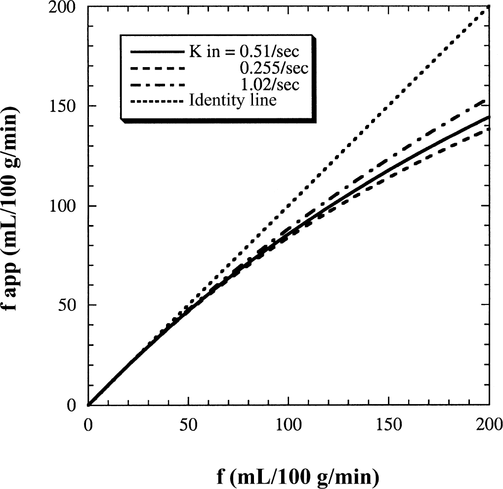
Effect of changing permeability surface area products on the calculated apparent magnetic resonance imaging flow values obtained with the conventional model from the FAIR signal-intensity difference plotted as a function of the true flows. The FAIR signal intensities calculated from the two-compartment model using k_in = 0.51 sec⁻¹ and k_out = 0.027 sec⁻¹ are represented by the solid line. The calculated apparent flow curves for doubled (dash-dotted curve) and halved (dashed curve) exchange rates due to changes in PS are plotted for comparison.

Finally, it is of interest to discuss the effect of hematocrit (Hct) on this issue, as Hct is dependent on the vessel diameter. The authors expect no influence of this, because all water in the blood (inside erythrocytes and plasma) is labeled completely and simultaneously, and the exchange between erythrocytes and plasma is very fast on the time scale of these experiments (erythrocyte lifetime is approximately 12 milliseconds (Herbst and Goldstein, 1989); experiment is on the order of 1 second).

Validation of the experimental results

It is important to investigate whether there are any confounding factors in the experiments that may adversely influence the conclusions about the need for using a two-compartment exchange model at higher flows. One potential problem is that a surface coil was used for both RF transmission and signal reception. This experimental setup leads to a restricted tagging volume and therefore a finite transit time, τ_d, for the trailing edge of the tagging bolus, because the NS measurements become partially selective. The authors previously estimated τ_d to be approximately 2.1 seconds during normocapnia (Zhou et al., 1998; Zhou and van Zijl, 1999a, b ). As flow increases at hypercapnia, τ_d is shortened and the labeling efficiency may be reduced, which is a potential source of error for the high flows. To test whether the hyperbolic secant pulse inverts a sufficient area of the brain and its feeding vessels, the authors performed an extra experiment in which the imaging profiles perpendicular to the coil were acquired at TI = 1.1 seconds for a range of at least 4 cm from the top of the brain by increasing the power of the imaging RF pulses, but keeping the sech pulse unchanged. In all cases, these profiles could be effectively nulled because of inversion at all distances up to at least 4 cm. Furthermore, it is known theoretically that flows quantified by the fitted FAIR signal-intensity differences at long TI (1.6 seconds) gradually become less than those quantified at short TI (1.2 or 1.25 seconds) as τ_d decreases and approaches 1.6 seconds. The experimental result of almost equivalent CBF numbers at the two TI values at all flow levels as shown in Fig. 7 implies that it is likely that τ_d was not decreased to be shorter than 1.6 seconds under all circumstances. Consequently, the shortening of τ_d is not a main problem for the measured flow range in this experiment setup. A final potential problem is the use of a very low b value (0.19 sec/mm²) for the flow-dephasing crushers to facilitate the presence of all microvascular signals in the experiments, as this is included in the authors' model. As a result, the flow-dephasing effects because of these crushers may be different at high and low flow, influencing the FAIR signal intensities at different flows. Although there is no certain way to confirm this, the authors expect this effect not to significantly influence their comparison of the apparent flows calculated for the two models. The reason is that the same signal intensities were used for interpretation with the single-compartment and the two-compartment model, which should make the relative effect small.

Conclusions

A theory was developed to describe the limited exchange of water between microvascular and extravascular space in the FAIR experiments. The equations presented are concise and can be reduced to the well-known expressions for the fast exchange limit (single-compartment model). Using the new two-compartment model, it was shown that the microvascular FAIR signal intensity is comparable in magnitude to the extravascular FAIR signal intensity, and that these two contributions are not overlapped in time, but that the former approaches its maximum earlier than the latter. When compared with the model of fast exchange, the total FAIR signal intensities from the two compartments are decreased and moved to shorter inversion recovery times. Theory also shows that the FAIR signal-intensity difference for flow quantification is independent of the length of the predelay between repeated measurements when assuming complete labeling between scans. It was found that apparent flow values quantified from the T₁ difference may be increased significantly because of the effects of short predelay and finite transit times of the tagging bolus in both models, but that the increased apparent flows are partially compensated by the effect of restricted water exchange. The experimental results on cat brain demonstrate that flows quantified from the signal-intensity difference are underestimated when the restricted exchange of water is erroneously taken as fast exchange, an effect that becomes more pronounced at higher flows. However, flows determined with the model taking into account the limited exchange of water are comparable with those determined by the radioactive microsphere technique. The theory outlined in the current article can be directly extended to other arterial spin labeling methods.

Finally, it is important to discuss the impact on human experiments. Because the authors used the human PS product for their calculations, the simulations and data can be compared quite directly. The simulations in Figs. 4 and 8 show that the effect becomes important above flows approximately 60 mL 100 g⁻¹ min⁻¹ at the current field strength of 4.7 T. However, most human experiments occur at a field strength of 1.5 T, in which the effects were not expected to be visible below flows of 90 to 100 mL 100 g⁻¹ min⁻¹. This situation will change with the present industrial trend of going to higher field (3 to 4 T) for human scanners, which will require inclusion of the exchange.