
Abstract
The present study determined cerebral blood flow (CBF) in the rat using two different magnetic resonance imaging (MRI) arterial spin-tagging (AST) methods and 14C-iodoantipyrine (IAP)-quantitative autoradiography (QAR), a standard but terminal technique used for imaging and quantitating CBF, and compared the resulting data sets to assess the precision and accuracy of the different techniques. Two hours after cerebral ischemia was produced in eight rats via permanent occlusion of one middle cerebral artery (MCA) with an intraluminal suture, MRI-CBF was measured over a 2.0-mm coronal slice using single-coil AST, and tissue magnetization was assessed by either a spin-echo (SE) or a variable tip-angle gradient-echo (VTA-GE) readout. Subsequently (∼2.5 hours after MCA occlusion), CBF was assayed by QAR with the blood flow indicator 14C-IAP, which produced coronal images of local flow rates every 0.4 mm along the rostral—caudal axis. The IAP-QAR images that spanned the 2-mm MRI slice were selected, and regional flow rates (i.e., local CBF [lCBF]) were measured and averaged across this set of images by both the traditional approach, which involved reader interaction and avoidance of sectioning artifacts, and a whole film-scanning technique, which approximated total radioactivity in the entire MRI slice with minimal user bias. After alignment and coregistration, the concordance of the CBF rates generated by the two QAR approaches and the two AST methods was examined for nine regions of interest in each hemisphere. The QAR-lCBF rates were higher with the traditional method of assaying tissue radioactivity than with the MRI-analog approach; although the two sets of rates were highly correlated, the scatter was broad. The flow rates obtained with the whole film-scanning technique were chosen for subsequent comparisons to MRI-CBF results because of the similarity in tissue “sampling” among these three methods. As predicted by previous modeling, “true” flow rates, assumed to be given by QAR-lCBF, tended to be slightly lower than those measured by SE and were appreciably lower than those assessed by VTA-GE. When both the ischemic and contralateral hemispheres were considered together, SE-CBF and VTA-GE-CBF were both highly correlated with QAR-lCBF (P < 0.001). If evaluated by flow range, however, SE-CBF estimates were more accurate in high-flow (contralateral) areas (CBF > 80 mL · 100 g−1 · min−1), whereas VTA-GE-CBF values were more accurate in low-flow (ipsilateral) areas (CBF ≤ 60 mL · 100 g−1 · min−1). Accordingly, the concurrent usage of both AST-MRI methods or the VTA-GE technique alone would be preferred for human studies of stroke.
The single-coil steady-state arterial spin-tagging (AST) technique (Detre et al., 1992; Williams et al., 1992) is the oldest magnetic resonance imaging (MRI) method that uses the protons of arterial blood as an autologous indicator for the measurement of cerebral blood flow (CBF). Theoretical aspects of this technique have been widely studied (Alsop and Detre, 1996; Ewing et al., 2001; McLaughlin et al., 1997; Pekar et al., 1996; Silva et al., 1994, 1997; Yeung, 1993; Zhang et al., 1992, 1993), but experimental validation in animals has been limited to one direct comparison between the steady-state AST technique and a microsphere measurement (Walsh et al., 1994). This paucity of correlative validation is important as the steady-state AST technique becomes widely used to examine clinically significant animal models of cerebral pathology. For instance, in our laboratory, single-coil AST has been used with an imaging technique for assessing the state of cerebral perfusion in a variety of rat models of ischemia (Jiang et al., 1997). Questions have been raised regarding whether it is advisable to eliminate signal from vascular spins, whether the technique produces signal linear in flow, and under what conditions the technique might produce an unbiased estimate of flow (Ewing et al., 2001). It was in this framework that we examined the operating characteristics of the AST-MRI measurement across a wide range of flows.
In the present study, CBF was measured in rats by two single-coil AST techniques approximately 2 hours after MCA occlusion, and the results were compared with local CBF (lCBF) rates measured minutes later using 14C-iodoantipyrine (IAP) quantitative autoradiography (QAR), a well-accepted but highly invasive technique. For the AST studies, both gradient-echo and spin-echo (SE) readings were used to assay tissue magnetization. The aim of the study was to determine: (1) if there was a correlation between CBF estimates produced by the two AST-MRI methods; (2) if CBF rates measured by either or both of the AST-MRI methods were concordant with those determined by 14C-IAP—QAR; and (3) if the AST-MRI methods yielded robust estimates of CBF.
THEORY
In single-coil AST, inflowing arterial protons are adiabatically inverted by the combination of a magnetic gradient oriented parallel to the direction of flow and an off-resonance continuous wave (CW) radio-frequency (RF) signal, which together provide a highly efficient inversion of flowing protons as they pass through a plane in the neck of the experimental animal. The control condition is obtained by changing the sign either of the gradient or of the RF offset in order to place the inversion plane equidistant on the other side of the imaging plane (i.e., outside the head).
Theoretical treatments (Alsop and Detre, 1996; McLaughlin et al., 1997; Pekar et al., 1996; Silva et al., 1997; Williams et al., 1992; Zhang et al., 1993) have modified the Bloch equations to account for the difference in T1 due to the flow into a tissue voxel. The statement of theory common to all presentations is that flow is proportional to the difference in equilibrium magnetization between the label condition with the inversion plane in the neck and the control condition with the inversion plane above the head:
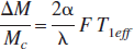
where ΔM = Mc - Mi, and:
Mi is the equilibrium magnetization with the arterial inversion plane in the neck,
Mc is the equilibrium magnetization with the inversion plane placed above the imaging plane (i.e., the equilibrium magnetization in the control condition),
α is the efficiency of inversion produced by the steady-state adiabatic inversion,
δ is the brain—blood partition coefficient for water (Herscovitch and Raichle 1985), set to 0.9,
F is the rate of cerebral perfusion, and
T1eff is the longitudinal relaxation time of the tissue measured under the conditions of the experiment, and in the presence of flow:
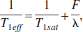
where T1sat is the T1 of the tissue water, measured under the condition of an off-resonance saturation of the macromolecular pool of the tissue protons. In the typical steady-state AST experiment, in which there is substantial magnetization transfer, the value of T1sat may be one half that of T1. In this relation, T1eff is thought to be only slightly dependent on flow. For a (high) flow of about 1.2 mL·g−1 ·min−1, and a T1sat of 0.5 second, this amounts to about a 2% change in T1eff, usually considered to be a negligibly small quantity.
We assumed that the macromolecular pool is essentially saturated, and that:
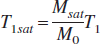
where M0 and T1 are proton density and longitudinal relaxation time under the conditions of no saturation. This tactic for the estimation of T1sat was used because of the superior signal-to-noise ratio of the three quantities on the right-hand side of Eq. 3.
MATERIALS AND METHODS
The suture model of middle cerebral artery occlusion in the rat
The origin of the MCA from the circle of Willis was occluded by an intraluminal suture to produce focal cerebral ischemia and a large range of CBF rates (Koizumi et al., 1986; Longa et al., 1989). Intraluminal suture occlusion of the MCA in the rat yields a reasonably reproducible, physiologically relevant animal model of stroke (Chen et al., 1992, 1993; Jiang et al., 1994).
Eight male Wistar rats weighing between 270 and 290 g were anesthetized with 3.0% halothane in a 2:1 mixture of N2O/O2 and maintained on 0.75% to 1.5% halothane. Body temperature was maintained at 37°C ± 0.5°C. The femoral arteries and veins were catheterized for arterial blood pressure recordings. The right common carotid, external carotid, and internal carotid arteries were exposed, and the proximal external carotid and occipital arteries were ligated. Another suture was loosely tied around the origin of the external carotid artery, and the common carotid artery was temporarily clamped with a microvascular clip. A 4–0 surgical nylon filament, whose length was adjusted according to weight and tip was made bulbous by holding it near a flame, was inserted into the lumen of the external carotid artery through a small incision and gently advanced into and up the internal carotid artery until it passed and blocked the origin of the MCA. After the incisions were infiltrated with lidocaine hydrochloride and closed, rats were immobilized in a holder that facilitated their positioning in the magnet.
To minimize stress, blood samples were not taken while the animals were in the magnet. A sample of blood was taken for blood gas analysis immediately on removal of the animal from the magnet and assumed to be representative of each animal's physiologic state at the times of MRI-CBF measurements. Another sample of blood, which was obtained just before infusing the radiotracer for the QAR estimation of flow, was analyzed for blood gases as well as glucose concentration, osmolality, and hematocrit.
Methods of magnetic resonance imaging measurement of cerebral blood flow
Steady-state AST creates contrast owing to perfusion by inverting the inflowing protons of arterial blood until a secular equilibrium is approached, where the inflow of the inverted protons is balanced by the loss of inverted protons via spinlattice interactions (T1 decay). The two single-slice MRI-CBF measurement techniques reported herein use different methods to read tissue magnetization. The first measurement technique, the original AST technique (Williams et al., 1992), uses paired SE images produced with and without the inversion of inflowing arterial protons, whereas the second technique uses a centrally encoded gradient-echo imaging technique with a variable tip angle (Ewing et al., 1995), again with and without a prior inversion of inflowing protons. We shall refer to the spin-echo method as SE-CBF and the gradient-echo technique as VTA-GE-CBF.
Magnetic resonance imaging hardware and animal preparation
Immediately after MCAO, the rat was placed in a 7-T 20-cm bore superconducting magnet (Magnex Scientific, Abingdon, U.K.) interfaced to an SMIS console (SMIS, Surrey, U.K.). A 12-cm self-shielded gradient set with maximum gradients of 20 G/cm and rise times of 200 microseconds, housing a 5-cm internal diameter quadrature birdcage coil, were used in this study.
The rat was positioned on its back in a nonmagnetic holder with its head rigidly held by ear bars and its brain centered in the imaging coil. The axial position of the rat was adjusted until the image slice was 5 mm caudal to the rhinal fissure with the head held in a flat skull position. Standard imaging parameters were as follows: field of view, 3.2 cm; slice thickness, 2 mm; and matrix, 128 × 64, with the exception that the matrix for SE-CBF measurements was reduced to 64 × 64. Acquisition of data proceeded essentially continuously for approximately 2 hours after MCA occlusion. Single-slice T1 maps via phase-incremented progressive saturation (PIPS) (Ewing et al., 1996) and MRI-CBF determinations were interspersed with the generation of multislice T2 and apparent diffusion coefficient of water maps. For both spin-tagging sequences, time-domain data were zero filled to 128 × 128, baseline corrected, and Fourier transformed. The magnitude image was calculated, and the tissue magnetization was estimated pixel-by-pixel from the image intensity.
Arterial spin-tagging and the SE-CBF technique
In both SE-CBF and VTA-GE-CBF measurements, an adiabatic inversion of inflowing arterial protons (Dixon et al., 1986) was accomplished via an axial gradient of ± 0.3 kHz/mm and a CW transmission from the imaging coil of approximately 0.3 kHz at a frequency offset of ±6 kHz, which placed the inversion plane 18 mm below the imaging plane and perpendicular to the common carotid arteries in the neck of the animal. In the SE-CBF technique, using the previously described MRI parameters, the inversion power was turned on for 1 second and shut off for approximately 20 milliseconds (repetition time [TR] to echo time [TE] = 1,020/20), during which time one SE line in k-space was acquired with a spectral width of 25 kHz. The inversion power was then turned back on until the next SE acquisition. The efficiency of arterial spin labeling, α, was estimated using techniques previously described (Zhang et al., 1993). Control studies used combinations of inversion gradient (_0.3 kHz/mm) and frequency offsets (±6 kHz) that put the inversion plane 18 mm above the imaging plane, usually beyond the nose of the animal. To balance off-resonance MTC effects, images were acquired in sets of four (a procedure that originated in our laboratory), with both CW frequency offset and inversion gradient sign permuted through all four combinations. Sixteen total images, in four sets of four images (Jiang et al., 1994, 1997), were taken over a period of approximately 17 minutes. Weak diffusion gradients were used (b = 10) to kill the signal from the large arteries. No timing delays were used for the clearance of the vascular signal (Alsop and Detre 1996).
The VTA-GE cerebral blood flow technique
In this technique, the AST inversion power was turned on before beginning the acquisition of a centrally encoded VTA-GE image. In addition to the previously described imaging parameters, the GE parameters were as follows: TR/TE, 11/5 milliseconds; NEX, 64; and spectral width, 50 kHz. To allow for the equilibration of inverted protons in the imaging plane, the inversion pulse was turned on for a period of 4.5 seconds preceding the production of each VTA-GE image. Images were again taken in sets of four permutations of CW frequency offset and inversion gradient sign. Total imaging time was approximately 8 minutes. A timing delay of about 150 milliseconds was used in order to allow for the partial clearance of signal from the large arteries. Note that in the SE experiment, balanced flow-spoiling gradients (essentially mild diffusion-weighting gradients) can be placed around the 180° pulse; however, in the gradient-echo experiment, flow-spoiling gradients are too costly in terms of time and the creation of unwanted eddy currents, and one must wait for the inverted signal to clear from the larger vessels.
Magnetization transfer, T1, and T1sat
The magnetization transfer properties of this rat model of cerebral ischemia, particularly under the conditions of the AST off-resonance pulse (6 kHz off-resonance, 0.3 kHz amplitude), have been reported previously (Ewing et al., 1998). A transfer of magnetization occurs at a considerable rate from the (MRI-visible) protons of the free water of the tissue to the (MRI-invisible) protons of the macromolecular and “bound water” proton pools. Under the conditions of the steady-state AST experiment, the magnetization (M0) and the T1 of the free water pool shorten to about half that observed with no off-resonance saturation. We call this decreased equilibrium magnetization Msat, and the shorter relaxation time T1sat, to distinguish these values from M0 and T1, the equilibrium magnetization and longitudinal relaxation times observed under the conditions of no off-resonance saturation. The values M0, T1, Msat, and T1sat were measured in the central imaging slice using PIPS (Ewing et al., 1996, 1998), a variant of TOMROP—t-one by multiple readout pulses (Brix et al., 1990).
Quantitative autoradiographic measurement of cerebral blood flow
Local CBF was measured by the 14C-iodoantipyrine technique developed by Sakurada et al. (1979) and modified by Otsuka et al. (1991). Using the previously cannulated blood vessels, an extracorporeal arteriovenous shunt was formed by connecting one arterial catheter to the venous catheter on the same side with a 1.5-cm piece of silicone tubing (Pharmacia Biotek, Arlington Heights, IL, U.S.A.). Blood gases, pH, blood glucose, and hematocrit values of blood samples drawn from the shunt immediately on removal from the magnet and again before infusing 14C-IAP were measured, and blood pressure was continuously monitored via the other femoral artery catheter. At the beginning of the experiment, approximately 50 μCi 14C-IAP (4-[N-methyl-14C]-iodoantipyrine; American Radiolabeled Chemicals, St. Louis, MO, U.S.A.) in 1.0 mL saline was infused with a variable-speed pump. The rate of infusion was increased according to a predetermined schedule, resulting in a linear increase of IAP concentration in the blood over the duration of the infusion. Arterial blood samples were obtained from the shunt at 5-second intervals by puncturing the silicone tubing with a 23-G needle on a heparinized, plungerless syringe. The time of sampling was considered to be the midpoint of each collection period (the latter was carefully measured). Rats were decapitated immediately after the last sample was collected, which was approximately 30 seconds after the IAP infusion was initiated.
Analysis of blood and brain samples
The 14C-IAP activity in blood samples was determined by liquid scintillation counting of plasma aliquots. Immediately after decapitation, the heads were dropped into 2-methylbutane chilled to −45°C and stored at −80°C until dissection. While working within a chest freezer set at −20°C, the brain with meninges and blood vessels attached was removed from the skull and maintained frozen, with CSF and blood trapped within their respective compartments. This procedure minimizes distortion of the brain and facilitates the comparison of the AST-MRI (premortem) and QAR (postmortem) images. The brain was covered with cold mounting medium and kept in a sealed plastic bag at −80°C until the time of sectioning. After warming in a −18°C cryostat for 30 minutes, the frozen brain was cut at 400-μm intervals into sets of five 20-μm-thick coronal sections. The first and last sections were stained with cresyl violet and used to identify regions of interest (ROIs) while the remaining three sections were picked up on coverslips, dried at 50°C on a hot plate, and prepared for autoradiography.
The dried brain sections and sets of commercially prepared methylmethacrylate 14C standards (American Radiolabeled Chemicals) were placed in cassettes with x-ray film (MR 2000–1; Kodak, Rochester, NY, U.S.A.), which was developed after 17 to 21 days of exposure. Blood flow was calculated from the autoradiograms by both the traditional method of Sakurada et al. (1979) and by an approach similar to that used for the MRI measurement. In both methods, background was estimated by reading optical density in a number of areas around the tissue images as well as in the lightest areas of the tissue images. The lowest optical density reading, usually found around the tissue images, was selected as background. This estimate of background was subtracted from all tissue and standard optical densities and resulted in lCBF values ≥0.0.
For the AST-MRI studies, flow was estimated in a 2.0-mm slab of tissue that extended from 0.2 to −1.8 mm relative to bregma. To make the autoradiographic data (obtained every 0.4 mm) match in space the 2.0-mm AST-MRI readings, five consecutive sections that spanned the latter were identified, and average radioactivities per ROI were estimated in one of two ways. In either case, a standard curve constructed from the 14C-standard data and a modified spline-fit routine was used to convert optical density to radioactivity.
With the traditional or field-by-field method (method 1), we measured and averaged on each of the selected autoradiographic images the optical densities in four to eight small artifact-free fields within each of the nine ROIs on both sides of the brain (Fig. 1) using an MCID image analysis system (Imaging Research, St. Catharines, Ontario, Canada). The average optical density was converted to radioactivity with the standard curve. The rate of blood flow was then calculated from the average radioactivity and the time course of 14C-IAP in arterial blood by the working equation of the method described by Sakurada et al. (1979). The equilibrium tissue-blood partition coefficient of IAP was set at 0.8 mL/g (Sakurada et al., 1979). This procedure was repeated for each of the five selected autoradiographic sections, and an overall mean CBF was calculated for each ROI. Method 1 avoids the most common artifacts of the 14C-IAP technique: small folds and tears in the tissue sections.
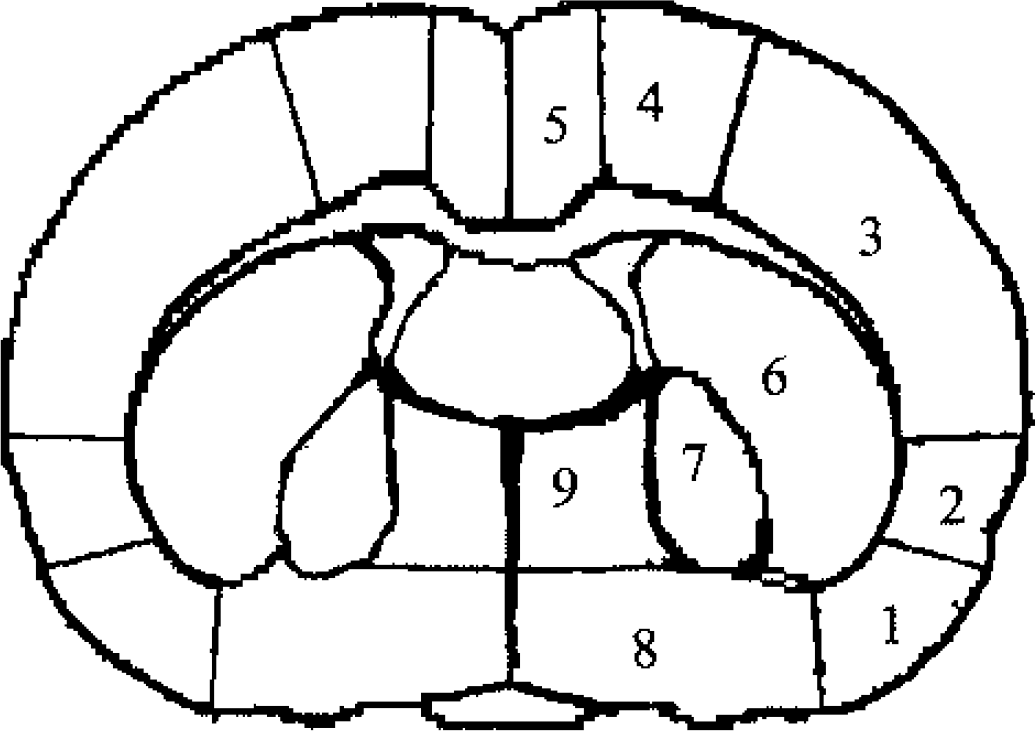
Diagrams of the 9 regions of interest (ROI) in which QAR-lCBF, SE-CBF, and VTA-CBF were estimated. These regions are: 1, piriform cortex (PiC); 2, insular cortex (InC); 3, parietal cortex (PaC); 4, hind-limb and forelimb cortex (HFC); 5, frontal and cingulate cortex (FCC); 6, caudate-putamen (Cpu); 7, globus pallidus (GlP); 8, preoptic area (PoA); and 9, midline nuclear structures of the stria terminalis (StT). QAR, quantitative autoradiography; SE, spin echo; CBF, cerebral blood flow; lCBF, local CBF; VTA, variable tip-angle.
In the second method (method 2), a standard radiologic film scanner (Lumiscan 75; Lumisys Corp, Sunnyvale, CA, U.S.A.) was coupled to home-written programs for the production of three-dimensional maps of tissue optical density and, in turn, of radioactivity across the entire MRI coronal slice including both ROIs and non-ROIs, artifacts and all. Subsequently, the program generated three-dimensional maps of blood flow for the whole 2.0-mm reconstructed slab of tissue. Then, a template of Fig. 1 that outlined the ROIs was laid over the final blood flow map, and mean flow for each ROI was determined.
Experimental assumptions and statistical analysis
All values are reported as the mean ± SD, and flow values are reported in mL · 100 g−1 · min−1. In the regression models, both simple regressions, which ignore the fact that multiple observations come from the same animals, and generalized estimating equation (GEE) (Liang and Zeger, 1986) models, which do take into account the correlation from the clusters of observations from the same rats, were performed. The simple regressions were performed to yield descriptive measures, especially correlation coefficients, which are not produced with GEE regression analysis, whereas the more formal GEE regressions were used to yield valid P values. Generalized estimating equation regressions were performed for each comparison of techniques (SE-CBF vs. QAR-CBF, VTA-GE-CBF vs. QAR-CBF, and SE-CBF vs. VTA-GE-CBF estimates), comparing measurements from each hemisphere separately. For each of the eight experiments, regressions were performed separately in the ischemic and nonischemic hemispheres. Comparisons of correlations were made separately within each rat using a method described by Yu and Dunn (1982). For an overall test of a difference, the eight correlation differences were compared by a Wilcoxon signed rank test. Thus, a comparison was available to reflect whether the MRI-CBF measurements agreed with QAR-CBF estimates under conditions of both ischemic flow and normal flow.
In both MRI techniques, the quantity M was estimated from the difference between the value of the summed magnitude images in the unlabeled condition minus the value of the summed magnitude images in the labeled condition (Eq. 1). When flow approaches zero, random and randomlike fluctuations in the magnitude images can produce negative values of flow. Since we have a priori knowledge that the true differences cannot be negative, we set all negative values of M to zero (Sijbers et al., 1998, 1999). This procedure was also followed in QAR estimates in the rare event that an area of film had a density lower than that produced by the mean value of the background estimate.
The significance of the differences in the means for each ROI between QAR data and either the VTA-GE or the SE data was determined with t-tests. The level of significance was set at P < 0.05 adjusted by Bonferroni correction.
RESULTS
The blood gas data (mean ± SD) obtained after the animals were removed from the magnet and before IAP infusion were as follows: PCO2 = 46 ± 10 and 48 ± 6 mm Hg; PO2 = 111 ± 38 and 95 ± 20 mm Hg; and pH = 7.38 ± 0.07 and 7.38 ± 0.03, respectively. The differences between these values were not significant. Before the start of the QAR measurement, blood glucose and osmolality were 188 ± 49 mg% and 309 ± 3 mOsm/L, respectively. Both values are higher than normal, and the high glucose level (10 mmol/L) accounts for much of the elevation in osmolality. Hematocrit (39 ± 5%) and mean arterial pressure (109 ± 8 mm Hg) values were normal before the QAR part of the experiment. Therefore, the physiologic state of the rats, though moderately hypercapnic and hyperglycemic, was otherwise fairly normal and was similar both inside and outside the magnet.
In Fig. 2, the QAR estimates of absolute flow rates by method 2 are plotted against those of method 1, the standard way of determining lCBF. The slope of the regression line is 0.57, showing that the QAR estimates of flow rate per ROI were generally lower using method 2, a discrepancy that may have resulted from individual readings of the film using method 1 (i.e., the darkest, most uniform fields within the ROI were chosen, avoiding edges where flow tended to be lower and eliminating the fields with artifacts). Method 2 eliminated user bias and averaged over the entire ROI, but might have suffered from partial volume effects at the edges and the inclusion of artifacts in the autoradiographic data within the reading template. Despite the differences in film-reading procedures, the values produced by the two methods were highly correlated (r = 0.89, P < 0.001). Because method 2 sets the boundaries of the ROI on the lCBF maps exactly as was done with the MRI-CBF maps, includes all of the tissue within the MRI-defined ROI, has partial volume effects as does MRI, and is similarly objective, the QAR-CBF data provided by the film-scanning method were used for comparison with MRI results. Figure 2 serves as an example of both the bias and the irreducible noise present in the procedure of coregistering and summing across tissue sections versus the selection of discrete fields for quantifying tissue radioactivity.
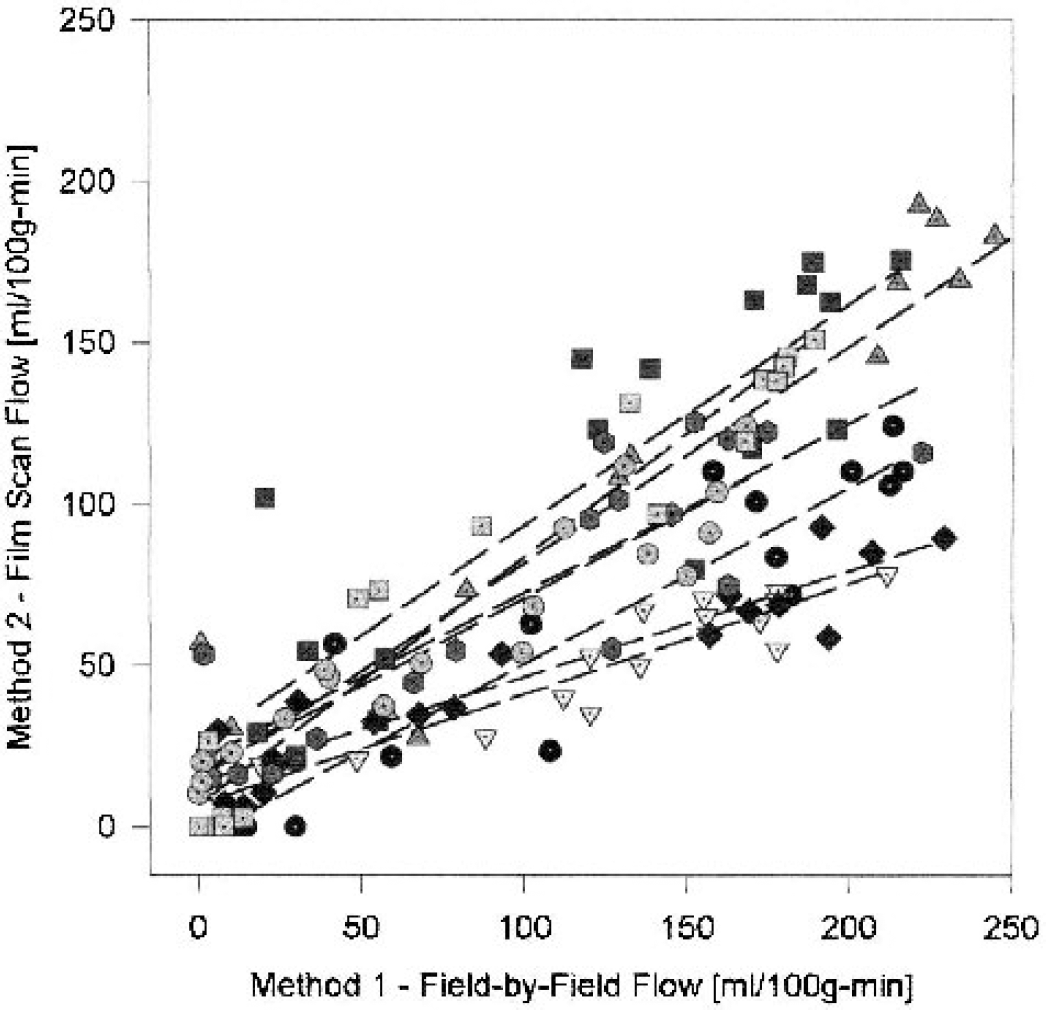
Comparison of the estimates of local cerebral blood flow (lCBF) made from the blood—brain distribution of 14C-iodoantipyrine (IAP) between two ways of assessing tissue radioactivity by quantitative autoradiography (QAR). Tissue radioactivity was assayed on the same set of autoradiograms by either whole film scanning and image summation (method 2) or traditional field-by-field reading and field averaging (method 1). Method 2 estimates of lCBF are plotted against method 1 evaluations of lCBF for 8 rats after approximately 2.5 hours of middle cerebral artery occlusion, 9 regions of interest (ROIs) per rat with both the ipsilateral (ischemic) and contralateral ROIs included (144 points). The dashed lines are the least square fits for the individual experiment including both ipsilateral (lower flows) and contralateral (higher flows) points. The flow estimates for each ROI obtained by the two methods are highly correlated, but those from method 2 are almost always less than those from method 1. Although derived from the same blood data and set of autoradiograms, the differences arise from technical variations such as exclusion (method 1) versus inclusion (method 2) of tissue section artifacts, partial volume effects (method 2), and different tissue-averaging procedures.
Both halothane (the anesthetic used in the present experiments) and hypercapnia (the physiologic condition in these rats) affect CBF. In accordance with these facts, the absolute rates on the contralateral side in the present group of animals appear to be higher than normal. For example, field-by-field—determined (method 1) mean lCBF rates for normal, awake rats (Bereczki et al., 1993) were compared with those for contralateral brain (method 1 in Fig. 2). For the four ROIs included in both studies, the mean ± SD rates (mL · 100 g−1 · min−1) were, respectively: 181 ± 27 and 197 ± 27 for the parietal cortex; 84 ± 36 and 150 ± 31 for the preoptic area; 78 ± 27 and 176 ± 37 for the globus pallidus; and 130 ± 15 and 204 ± 39 for the caudate-putamen. For these four ROIs, the lCBF values in the hypercapnic, halothane-anesthetized rats used in the present study were both higher and more uniform than corresponding values found in awake controls. It is possible that these conditions have some effect on CBF in the various ROIs on the ischemic side, but they probably do not affect the comparisons in the flow data produced by the several techniques.
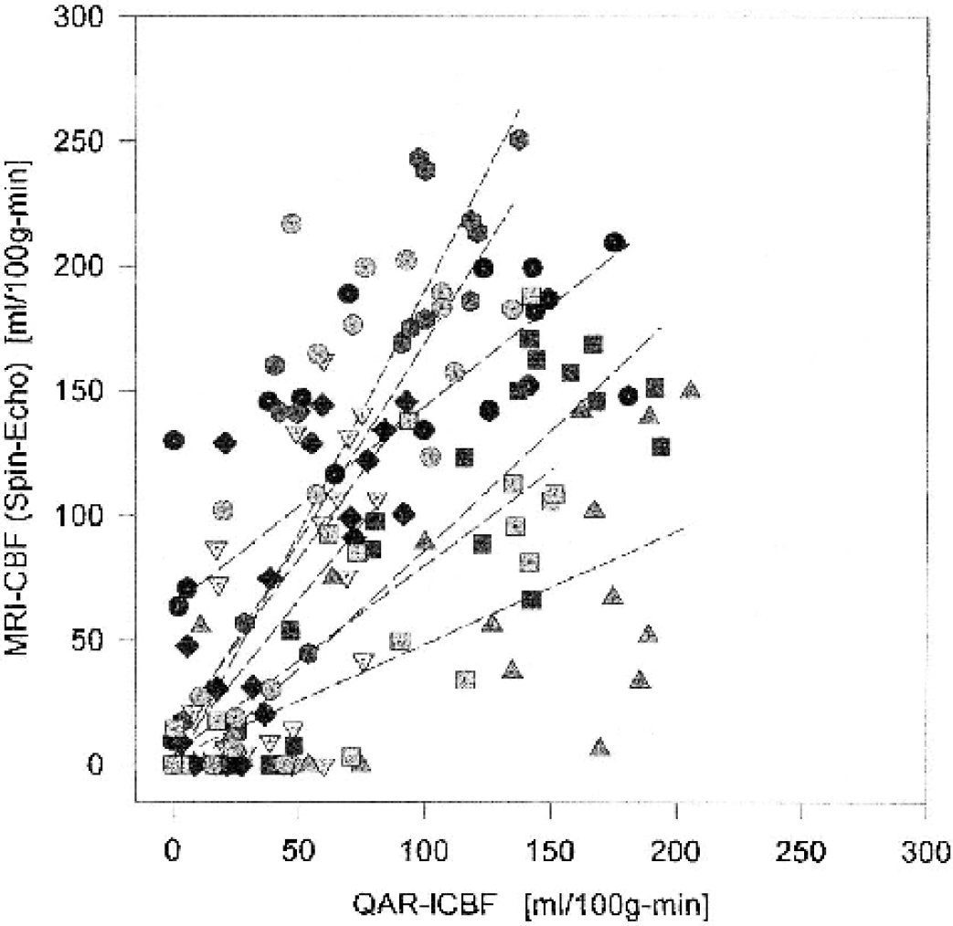
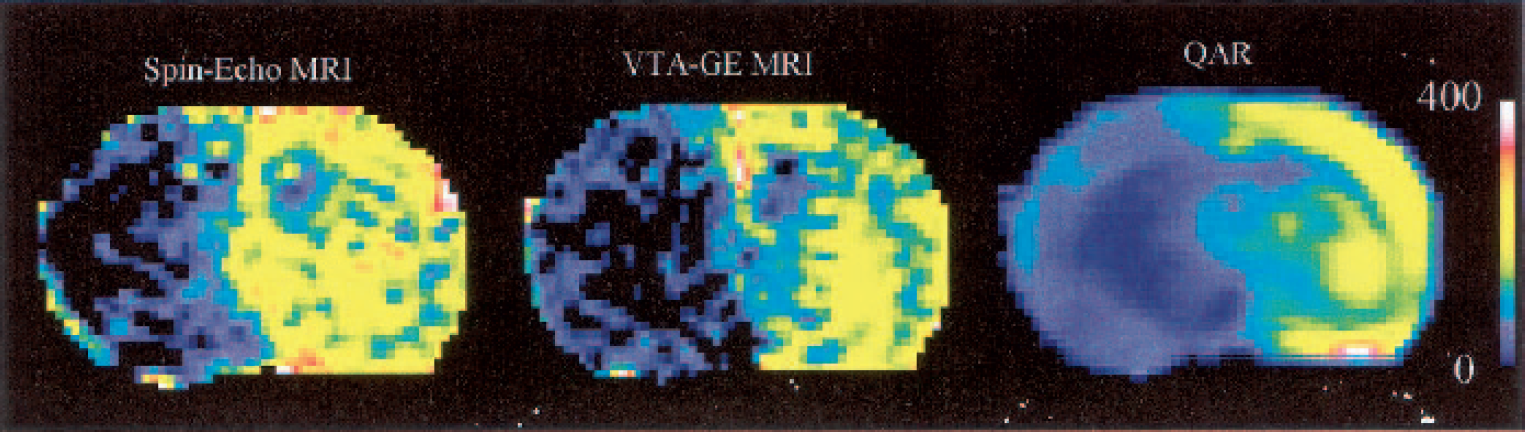
For the group of eight rats, inversion efficiency (a in Eq. 1) was measured as 0.90 ± 0.05. The maps of absolute flow rates generated by the two MRI techniques appeared well matched and closely resembled those obtained by QAR (example maps in Fig. 3). The lCBF estimates ranged from essentially zero to nearly 200 for QAR and zero to 250 for SE-AST (Fig. 4). The scatter of points was considerable. For instance, at QAR-lCBF roughly equal to zero, SE-CBF varied from 0 to 130, and at QAR-lCBF = 100, SE-CBF ranged from 80 to 250. Incidentally, in the lCBF range of 90 to 200 mL · 100 g−1 · min−1 (abscissa in Fig. 4), most of the points are from the contralateral side, and the spread in these data is huge, in part owing to some very low SE-CBF rates. However, GEE analysis indicated a positive correlation (slope = 0.191, P < 0.001) between SE-CBF and QAR-lCBF measurements in the ischemic hemisphere. For the contralateral, nonischemic hemisphere, where the range of individual SE-CBF values was very large, the correlations were not evident (slope = 0.044, P = 0.416). When both hemispheres were included in the GEE analysis, there was a stronger positive correlation between the two measurements (slope = 0.480, P < 0.001). Therefore, agreement was fairly good between the two sets of CBF data, and estimates of the absolute flow rates tending to be higher for SE-MRI than for QAR.
The flow maps for a 2-mm-thick coronal slice from one derived from each of the three techniques of reading tissue signal; spin-echo (SE) magnetic resonance imaging (MRI;
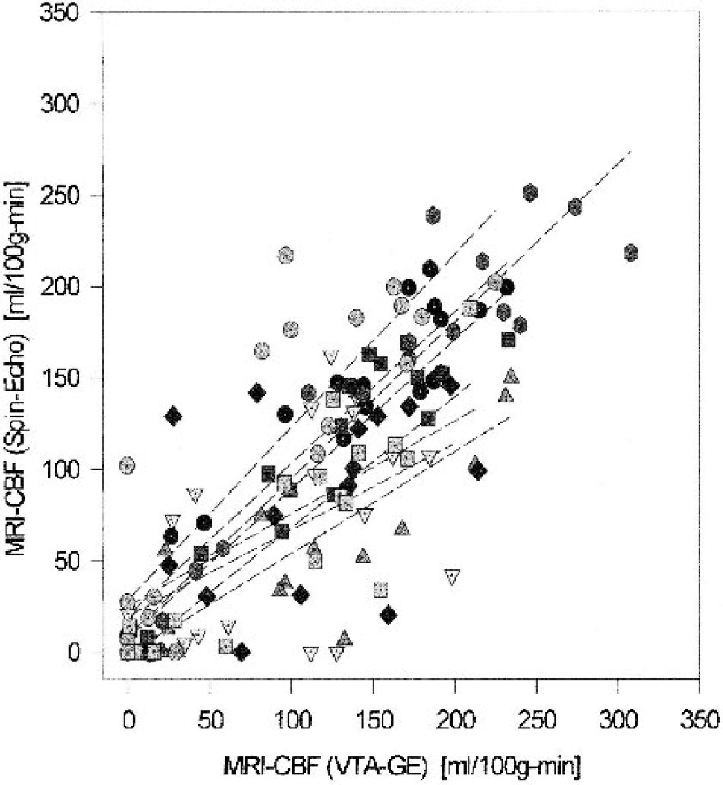
SE-CBF versus QAR-lCBF estimates of blood flow plotted for each region of interest (ROI) from both sides of the brain, 9 ROIs, and 8 rats (144 points). The dashed lines are the least square fits for the individual experiment for both ipsilateral (lower flows) and contralateral (higher flows) points. The flow estimates for each ROI obtained by the two methods are highly correlated, but these data scattered broadly. At QAR-lCBF ≤ 60 mL · 100 g−1 · min−1 (mild to severe ischemia), many of the magnetic resonance imaging (MRI)-CBF rates were zero and many others were > 60mL · 100g−1 · min−1. At higher flow rates (mainly normal tissue), however, SE-CBF was higher than QAR-lCBF in approximately two of three cases. SE, spin-echo; CBF, cerebral blood flow; lCBF, local CBF; QAR, quantitative autoradiography.
Similar to the preceding comparison (Fig. 4), the absolute flow rates estimated by VTA-GE-CBF were mostly higher than those measured by QAR (Fig. 5); the scatter in the data, however, appears to be less in Fig. 5 than in Fig. 4. Especially notable was that in the 90- to 200-mL · 100 g−1 · min−1 lCBF range (mostly contralateral-side data), there were very few low VTA-GE-CBF points (Fig. 5). Moreover, in the QAR-lCBF range of 0 to 25 mL · 100 g−1 · min−1, 18 of 27 VTA-GE-CBF rates were in the same range, and the agreement in absolute flow rates was fairly good. Overall, there was a strong positive correlation between the estimates of flow between the two methods for the ischemic side (slope = 0.340, P < 0.001), the nonischemic side (slope = 0.216, P < 0.001), and the two sides taken together (slope = 0.500, P < 0.001).
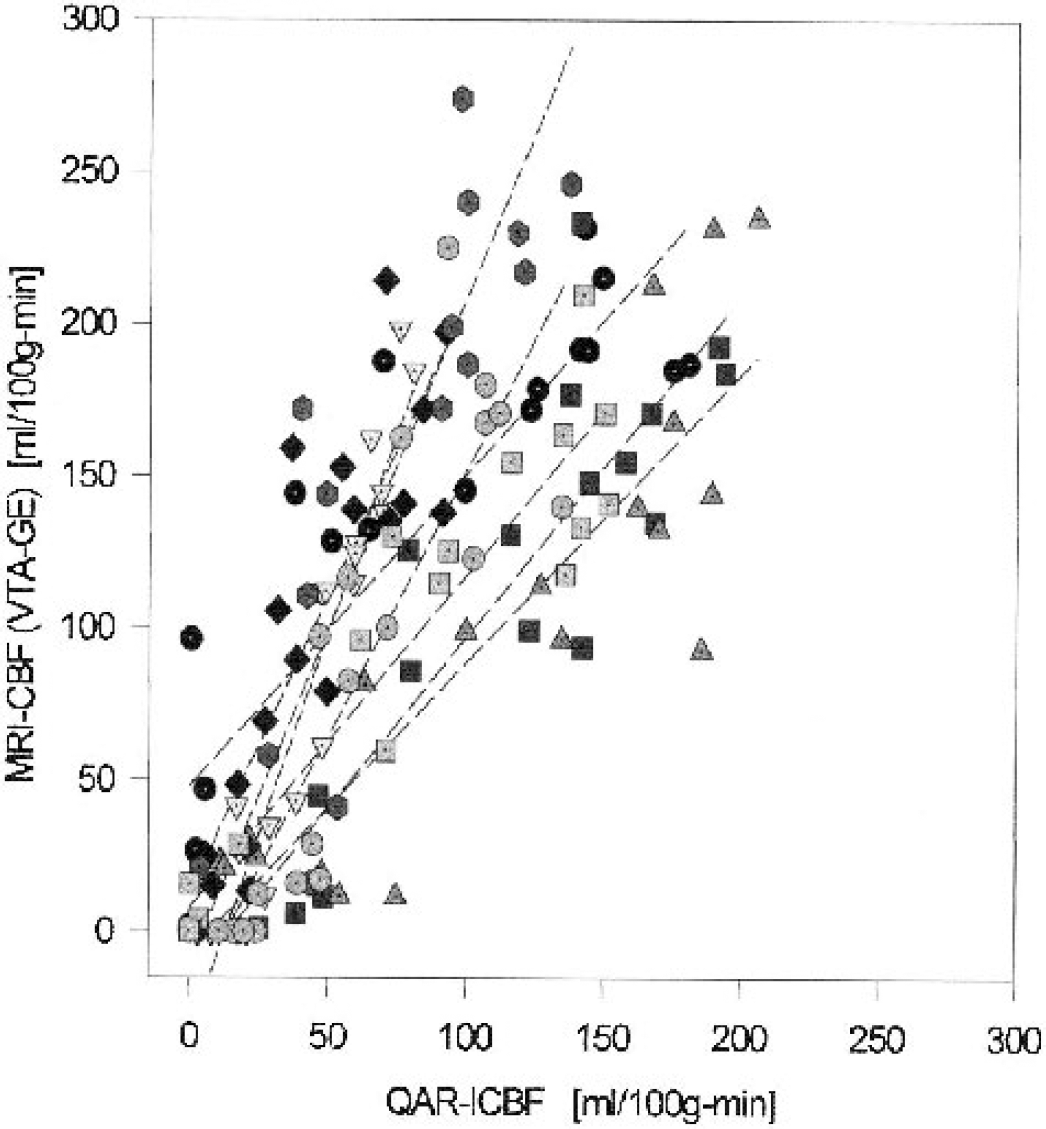
VTA-GE-CBF versus QAR-lCBF estimates of blood flow plotted for each region of interest (ROI) from both sides of the brain, 9 ROIs, and 9 rats (144 points). The dashed lines are the least square fits for the individual experiment for both ipsilateral and contralateral points. The flow estimates for each ROI obtained by the two methods are highly correlated. Noting that the QAR-lCBF data are the same in Figs. 4 and 5 and that the scaling is the same in both, the scatter of the points can be seen by visual inspection to be less for the VTA-GE plot (Fig. 5) than the SE plot (Fig. 4). At QAR-lCBF ≤ 25 mL · 100 g−1 · min−1, most of the VTA-GE data also fall in this range and suggest severe ischemia. In contrast, at higher flow rates (mostly contralateral, normal tissue), VTA-GE-CBF was almost always higher than QAR-lCBF for each ROI. MRI, magnetic resonance imaging; VTA-GE, variable tip-angle gradient-echo; CBF, cerebral blood flow; lCBF, local CBF; QAR, quantitative autoradiography; SE, spin-echo.
Flow by VTA-GE-CBF (Fig. 5) was more highly correlated with QAR-lCBF than was SE-CBF (Fig. 4); the nominal correlations with the QAR-determined flows were 0.78 for the gradient-echo method and 0.59 for the SE technique. To further examine the capability of the MRI methods to estimate regional flows, separate correlations were performed for each rat. In five of eight rats, the correlation with QAR-measured blood flow was significantly higher with VTA-GE-CBF than with SE-CBF, and higher gradient-echo correlations were also found in the remaining three rats, even though the differences were not statistically significant. The Wilcoxon signed rank test P value for the eight correlation differences was 0.008.
As for differences between the flows estimated by the two AST-MRI methods, the CBF rates measured by SE-MRI were generally lower than those determined by VTA-GE (Fig. 6), but the scatter in the data was considerable. As might be expected because of the similarity in reading the tissue signal and time of measurement, the correlation between VTA-GE-CBF and SE-CBF estimates was stronger than that found between either AST method and QAR-lCBF. In the ischemic hemisphere (P < 0.001), nonischemic hemisphere (P = 0.039), and both hemispheres combined (P < 0.001), the correlations were robust and significant, although considerably less so for the nonischemic hemisphere.
SE-CBF versus VTA-GE-CBF compared for 8 rats and 9 regions of interest (ROIs) for both ipsilateral and contralateral hemispheres. Regression lines for each experiment are indicated by the dashed lines. At blood flow rates of 0 to 50 mL · 100 g−1 · min−1, SE-CBF was either similar to or slightly higher than the VTA-GE-CBF, but at higher flows SE-CBF was mostly either similar to or less than VTA-GE-CBF. Statistical testing indicated that overall SE-CBF was significantly lower than VTE-GE-CBF (<0.001 for both hemispheres combined). MRI, magnetic resonance imaging; CBF, cerebral blood flow; lCBF, local CBF; VTA-GE, variable tip-angle gradient-echo; SE, spin-echo.
To view the preceding data in a different way, the flow values were grouped by technique and ROI, ipsilateral—contralateral ratios formed, means and standard deviations calculated, and the significance of the differences examined. Mean regional flow values (n = 8) on the contralateral side were higher in most of the ROIs for the VTA-GE technique than for QAR (Fig. 7A), but were nearly identical for QAR and SE-MRI for six of the nine regions. The differences in the other three ROIs, however, were large (>50 mL · 100 g−1 · min−1). In general, the standard deviations of the three estimates of flow were similar for each of the nine regions. The differences in the contralateral side mean flow rates were not significant for any of the nine ROIs for QAR-lCBF versus VTA-GE-CBF or SE-CBF (P > 0.05, Bonferroni corrected, for all ROIs).
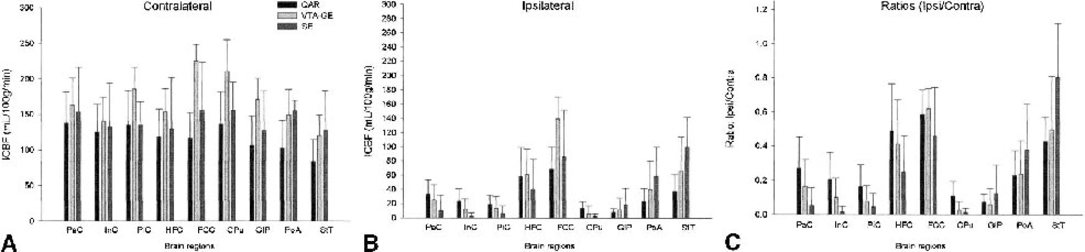
Mean (± SD) of the blood flows estimated by the three techniques for the 9 regions of interest (ROIs [see Fig. 1 for definitions of ROIs]).
On the ischemic side, the mean flow rates measured by QAR were less than 20 mL · 100 g−1 · min−1 for the piriform cortex, caudate-putamen, and globus pallidus (Fig. 7B) and fell between 22 and 37 mL · 100 g−1 · min−1 for the parietal and insular cortices, preoptic area, and stria terminalis. For all nine ROIs of the ipsilateral hemisphere, mean CBFs obtained with the two AST-MRI methods were not consistently larger or smaller than those with QAR. The standard deviations were large in many instances, and the differences in regional flow rates among the three approaches for the ipsilateral regions were not statistically significant (P > 0.05, Bonferroni corrected, for all ROIs). Therefore, mean flow rate estimates within ischemic ROIs appeared to agree fairly well among the techniques.
In many studies of blood flow and focal cerebral ischemia, the ipsilateral—contralateral ratios are reported. Such ratios for the QAR data ranged from less than 0.1 for the globus pallidus to 0.6 for the frontal-cingulate cortex (Fig. 7C); QAR-lCBF ratios of less than 0.3 were found in six of the nine ROIs. The VTA-GE-AST flow ratios in all nine regions were closer to the QAR ratios than the SE-AST flow ratios and seemed to approximate the QAR-lCBF flow ratios, the assumed benchmark. Although the differences in the ipsilateral—contralateral ratios between the QAR and either AST-MRI method for each ROI were generally sizable (Fig. 7), they were not statistically significant (Bonferroni-corrected P > 0.05 for all ROIs).
DISCUSSION
Maps of MRI-CBF obtained by two noninvasive techniques were directly compared with a profoundly invasive—but widely used—quantitative measurement of flow in the same animals. Across the brain and in the ischemic hemisphere, MRI-CBF was significantly correlated with QAR-lCBF. The CBF estimates obtained with the two AST-MRI methods varied widely compared with QAR estimates but tended to be higher at higher flow rates than the QAR values. Some of this discrepancy may be due to the film-scanning method of reading and subsequently averaging the spanning set of autoradiographic images and ROIs. This autoradiographic method yields lower CBF rates than does the traditional frame-by-frame approach. Furthermore, because times of measurement differed by 15 to 30 minutes, blood flow in some or all of the ischemic regions may have further decreased during the period between AST-MRI readings and QAR-lCBF measurements.
Comparisons of the arterial spin-tagging methods
That the VTA-GE technique produces higher estimates of lCBF than the SE method can be explained in its entirety by the higher capillary content of inverted protons with the former approach. Modeling of the SE-AST technique for the conditions of the current experiments (Ewing et al., 2001) has indicated that the inverted spins in the microvasculature supply a significant amount of the flow signal—as much as 30% in typical normal tissue. This result was dependent on TR, microvascular volume, and, most importantly, on the permeability of the microvasculature to water. The modeling led to a prediction that, in normal tissue, SE-CBF estimates would be higher than the actual flow. In cerebral tissue with normal capillary permeability to water, the model predicted that the ratio of MRI-CBF to true CBF would lie between 1.24 and 1.41; our measurements generally yielded ratios in that range for the nonischemic hemisphere, which is remarkable because the main experimental biases in this technique (i.e., loss of arterial signal due to transit between carotids and the tissue, magnetization transfer in the blood, and less than infinitely high permeability of the blood—brain barrier to water) tended to underestimate actual flow values. According to the modeling, overestimation of flow only arises from the difference in the relaxation times between blood and brain tissue and the presence of venous, capillary, and arterial blood in the voxel of interest. Since the SE-measured rates of flow appeared to be somewhat higher than those of QAR-lCBF, the microvascular signal in the single-coil AST experiments appears to be a source of systematic error large enough to produce an overestimation of the actual flow.
The capillary and small-vessel signal can be expected to have an even stronger effect on VTA-GE than SE measurements of flow. The VTA-GE sequence produces an image in about 700 milliseconds; for much of that time, inverted spins continue to flow into the imaging slice and thereby refresh the partially saturated spins that are already present. Although we have not modeled this situation in detail, the results of our measurements clearly reflect this excess of flowing spins; the VTA-GE estimates of flow were higher than either the SE (Fig. 6) or QAR (Fig. 5) rates. Of considerable interest is the possibility of using this property to yield an index of the cerebral blood volume in the imaging slice. For instance, the ratio of VTA-GE CBF to SE-CBF will yield a number that reflects the degree to which vascular spins are overcounted by the VTA-GE sequence.
It is a characteristic of the SE-CBF technique that all magnetization in the slice is destroyed by crusher gradients placed at the end of the read gradient. At the end of each line in k-space, therefore, the experiment essentially starts over again with zero magnetization in the tissue and a column of inverted protons being delivered to the microvasculature. This is not the case for the VTA-GE technique, where the sequence is so designed that the last-read pulse samples the last of the remaining magnetization. For each line in k-space, a partial readout of both tissue and vascular magnetization takes place. During the experiment, inverted protons continue to flow into the imaging slice, replenishing the vascular component and, to a lesser extent, the tissue component of inverted protons. Therefore, the VTA-GE-CBF technique emphasizes the vascular component of inverted protons even more than does SE-CBF; accordingly, this and other techniques that use fast gradient-echo readouts are microvascular volume-weighted flow measurements.
In both the SE-CBF and VTA-CBF methods, the experiment is designed so that only the local tissue magnetization varies between the “tag” and control conditions. This is done to create a condition in which the difference in tissue magnetization between tag and control is proportional to the product of flow and T1eff (Eq. 1). To a first approximation, therefore, the method used to read out tissue magnetization in a steady-state AST experiment should be a matter of indifference as long as the imaging method does not differ between tag and control state. Both methods of readout, the conventional SE technique with a 1-second TR and the gradient-echo technique optimized for signal intensity and with a 5-second TR, should yield equally accurate assays of tissue magnetization.
In comparing the two AST-MRI techniques, the steady state may be questioned for the SE estimation of flow, given the 1-second TR of the SE-CBF measurement. The effective T1 of the experiment is the T1 under the conditions of off-resonance saturation of the immobile protein pool of the tissue. With a 7-T magnet, T1sat shortens to about 0.5 seconds in most cerebral tissue, making the 1-second TR of the SE approach approximately twice that of the effective T1 of the experiment. Thus, even with the relatively short TR of 1 second, the steady state is approached (steady-state magnetization = 86% of the beginning magnetization) for the SE-CBF approach. Given a TR of 5 seconds, a steady state is more than 99% achieved for the VTA-GE method. This small difference in the approach to a steady state is not likely to contribute appreciably to the dissimilarity in the estimates of flow by the two techniques, but it must be added, in qualification, that this treatment ignores the contribution of the inverted protons residing in the microvasculature.
To pursue the latter point further, if the inverted protons residing in the microvasculature were not counted in the SE experiment, there would be a significant underestimation of flow to the tissue, not only because of the small saturation of the tissue but also because of the limited permeability of the microvasculature to water. Detailed modeling of the system (Ewing et al., 2001) has shown that an essentially linear response between magnetization and flow is achieved under the conditions of this experiment and for a wide range of physiologic parameters since both the microvascular population and the tissue population are included in the tissue readout. Thus, a 1-second TR, while not entirely achieving the steady state, does result in an approximately linear relation between the voxel population of inverted protons and the flow into that voxel.
A constant brain—blood partition coefficient for water of 0.9 was assumed during the processing of both sets of AST-MRI data. In fact, the partition coefficient for water can vary slightly from region to region in normal brain, and also in ischemic and edematous brain (Herscovitch and Raichle, 1985); the range of variation is from 0.9 (normal) to about 1.0 in edematous white-matter. In the rat model of permanent MCA occlusion used herein and the time period used in our studies (i.e., 2.0 to 2.5 hours after occlusion), there may be a small accumulation of tissue water that chang es T1sat across the time of the experiment (Ewing et al., 1999). T2, however, usually considered diagnostic of edema, did not significantly change (data not shown). Thus, whereas the partition coefficient may vary across the brain and lead to a slight overestimation of flow in the ischemic hemisphere, we do not believe that this effect is measurable, and is almost certainly less than 5% for both AST techniques.
Accuracy of the arterial spin-tagging techniques
Flow estimates by VTA-GE were apparently greater than those measured by SE or QAR. For both sides of the brain combined and for the ischemic hemisphere alone, flows estimated by both AST methods were significantly correlated with QAR-CBF; the correlation was, however, better for the VTA-GE than the SE technique and the individual data points much less scattered (Fig. 5 vs. Fig. 4, respectively). In the nonischemic, high-flow hemisphere, only the VTA-GE-CBF was significantly correlated with QAR-CBF. The combination of halothane anesthesia and hypercapnia seemingly increased CBF in nonischemic brain tissue and reduced the rate differences among the contralateral brain regions. This “smoothing out” of lCBF variations may have contributed to the lack of dynamic range encountered in the normal hemispheres of our experimental animals. Given this lack of dynamic range, the superior signal-to-noise ratio of the VTA-GE-CBF technique apparently resulted in a good correlation between the flows measured by QAR and VTA-GE even in the nonischemic hemisphere, whereas the poorer signal-to-noise ratio of the SE-CBF technique thwarted a significant correlation on the contralateral side.
The sources of experimental error in these comparisons of blood flow estimates among these several techniques originate not only in the measurements themselves but also in the procedures necessary to coregister and perform their comparison. It is notable that the two MRI methods that are coregistered in vivo and are taken almost concurrently, thus under the most uniform conditions, produce highly correlated measurements (Fig. 6). This is not the case for the comparison of the MRI-CBF data with QAR-measured flow rates. In slicing the brain for autoradiography, the sections were cut as close to parallel as possible to the MR imaging plane, which varied somewhat from animal to animal. The MR imaging plane of the magnet had to be located among the autoradiographic images, and the five (one set every 400 μm) that spanned the 2-mm MRI slice had to be coregistered with the MRI-CBF map. It also had to be assumed that the five autoradiographic data sets could be averaged with equal weights to correspond to the data of the MRI-CBF map. Finally, the physiologic state of each animal was assumed to be the same during all three sets of CBF measurements. One or more of these assumptions could be false and may have contributed to the scatter observed among the correlations between MRI and QAR data.
Given the proceeding experimental shortcomings, a moderate amount of noise in the scatter plots of the SE-CBF versus QAR-CBF and VTA-GE-CBF versus QAR-CBF measurements was expected and found (Figs. 4 and 5). The degree to which sources of noise was due to the procedures of the comparison (rather than due to the errors of the measurements) is not easily evaluated, but may be judged from a comparison of Fig. 6 (SE-CBF vs. VTA-GE-CBF), in which there is literally no error in coregistration, with Fig. 4 (SE-CBF vs. QAR-CBF), in which there are both methodologic and coregistration errors.
On the ischemic side of the brain, VTA-GE-CBF rates were fairly close to those measured by QAR-lCBF when the latter was ≤60 mL · 100 g−1 · min−1 (Figs. 5 and 7B). This finding suggests that this AST-MRI method produces better estimates of flow in ischemic areas than does SE-CBF. In contrast, the SE-CBF method yields flow rates in the higher-flow areas of the contralateral hemisphere (CBF > 80 mL · 100 g−1 · min−1) that correlate more strongly with QAR-lCBF than does the VTA-GE method (Figs. 4 and 7A). This difference between the ranges of “fit-to-QAR” for the two AST methods indicates that the VTA-GE will yield better estimates for low-flow areas and studies of ischemic tissue, whereas the SE will generate better estimates for high-flow areas and conditions that increase flow.
The bar graph of mean ipsilateral—contralateral flow ratios (Fig. 7B) is similar to that representing mean ipsilateral flow (Fig. 7C), which indicates that either treatment of the AST-MRI mean data produces similar results. Plots of the ipsilateral—contralateral flow values, however, were exceedingly large (ratios not shown) and showed virtually no correlation between either of the AST-MRI techniques and QAR-lCBF. The absolute AST-derived flow rates per ROI are, therefore, much more valuable than the ipsilateral—contralateral ratios for both experimental and human studies.
Our findings are somewhat at variance with those of Walsh et al. (1994), the only other published comparative study, who used the steady-state AST technique at 2.0 T and the radiolabeled microsphere method, another invasive technique. In their study, a volume-selective spectroscopic, rather than an imaging technique, was used, and thus only one relatively large piece of tissue was available per rat for comparison. Fairly good agreement among the paired measurements of blood flow was found, and MRI-CBF did not appear to overestimate flow relative to microsphere-measured CBF. There was, nonetheless, a tendency to underestimate flow in ischemic tissues using the steady-state AST technique visa-vis the microsphere technique. The authors attributed this disparity to the long arterial transit times between the inversion point and the sampling point in the ischemic brain areas, along with the relatively short T1 of blood at 2 T. The longer T1 of blood at 7 T found in the present experiments may reduce the effect of increased arterial transit time in low-flow areas and partially explain the differences in the AST data between the two studies.
To summarize, even though VTA-GE-CBF produced higher values, the rates found were somewhat better correlated with the “gold standard” QAR-lCBF values than were the SE-CBF rates. If evaluated by flow range, however, SE-CBF estimates seem to be better in high-flow areas (CBF > 80 mL · 100 g−1 · min−1), whereas VTA-GE-CBF values appear to be better in low-flow areas (CBF ≤ 60 mL-100 g−1 ·min−1). Accordingly, the concurrent usage of both AST-MRI methods would be preferred for human studies. For animal studies with a reproducible model of ischemia and groups of eight or more, mean CBFs per ROI reduce the differences and scatter in the flow data among the techniques. For nonterminal, repeated-over-time measurements in the same group of animals, either AST-MRI approach appears to work reasonably well and yield fairly good mean flow rate estimates. In this case, ipsilateral—contralateral ratios of AST-MRI data will produce useful relative flow information but not absolute flow values.
Footnotes
Acknowledgments
The authors thank Martin Gorski for his skilled technical assistance during the experiments, and Ms. Grenae Mosely for her help in manuscript preparation.