Sage Journals: Discover world-class research

Abstract

A quantitative estimate of cerebral blood oxygen saturation is of critical importance in the investigation of cerebrovascular disease because of the fact that it could potentially provide information on tissue viability in vivo. In the current study, a multi-echo gradient and spin echo magnetic resonance imaging sequence was used to acquire images from eight normal volunteer subjects. All images were acquired on a Siemens 1.5T Symphony whole-body scanner (Siemens, Erlangen, Germany). A theoretical signal model, which describes the signal dephasing phenomena in the presence of deoxyhemoglobin, was used for postprocessing of the acquired images and obtaining a quantitative measurement of cerebral blood oxygen saturation in vivo. With a region-of-interest analysis, a mean cerebral blood oxygen saturation of 58.4% ± 1.8% was obtained in the brain parenchyma from all volunteers. It is in excellent agreement with the known cerebral blood oxygen saturation under normal physiologic conditions in humans. Although further studies are needed to overcome some of the confounding factors affecting the estimates of cerebral blood oxygen saturation, these preliminary results are encouraging and should open a new avenue for the noninvasive investigation of cerebral oxygen metabolism under different pathophysiologic conditions using a magnetic resonance imaging approach.

Keywords

BOLD Cerebral blood oxygen saturation Magnetic resonance imaging

Clinical outcomes from a hypoxic or ischemic insult are a function of the magnitude and duration of diminished oxygen delivery to the brain (Heiss et al., 1983; Jones et al., 1981; Plum et al., 1986). The pathophysiology of altered oxygen delivery and oxygen demand can be viewed as a highly dynamic process (Grotta et al., 1986; Heiss et al., 1994). These fundamental insights have broad implications for a wide variety of disorders that involve or may involve abnormal cerebral oxygen delivery and oxygen demand, such as ischemic stroke, cerebral trauma, and shock. The most direct (and therefore optimal) measure of the balance between oxygen supply and demand is a measure of the cerebrovenous oxygen content, Cvo₂ (Siesjo, 1978), which represents the remaining oxygen dissolved in plasma and the residual saturation of venous hemoglobin. Because there is a minimal barrier to oxygen diffusion, Cvo₂ reflects the amount of delivered oxygen that is not consumed by the brain. This relationship is maintained even under clinically relevant low flow conditions (Sharan et al., 1989). For these reasons, many investigators have developed methods for measuring the Cvo₂, or the partial pressure of oxygen in venous blood (Pvo₂), from within the venous sinuses or jugular system (Cruz et al., 1990; Cruz, 1988, 1993; Bullock et al., 1993). However, these methods are invasive in nature and carry certain risks preventing them from being widely used in a daily clinical setting.

With the advent of fast imaging techniques and the improved understanding of the biophysical basis of blood-oxygen level dependent (BOLD) (Ogawa and Lee, 1990a; Ogawa et al., 1990b,c,1993a,b) contrast mechanisms, magnetic resonance imaging (MRI) now has the potential for studying the pathophysiology of disordered brain oxygen metabolism. Specifically, it has been demonstrated that when the concentration of deoxyhemoglobin is increased, a decrease in T2 and T2* is anticipated, resulting in a decrease in MR signal intensity in T2- and T2*-weighted images and vice versa. With animal models many investigators demonstrated that BOLD effects can be used to monitor the changes of oxygen saturation in vivo under pathophysiologic conditions, such as hypoxia (Turner et al., 1991; Prielmeier et al., 1994; Jezzard et al., 1994; Hoppel et al., 1993; Rostrup et al., 1995; Kennan et al., 1997; Lin et al., 1998a), hyper- and hypocapnia (Jezzard et al., 1994; Davis et al., 1998; Lin et al., 1999), hemodilution (Lin et al., 1998b), and ischemia (De Crespigny et al., 1992; Ono et al., 1997). However, all of the above studies only focus on relative measurements of cerebral blood oxygen saturation (Y) and little attention has been given as to how an absolute measurement of Y can be obtained with the BOLD effects.

Recently, with ex vivo blood samples and in a range of physiologically relevant oxygen saturation, both Wright et al. (1991) and Foltz et al. (1999) demonstrated that a calibration curve could be obtained between T2 of the blood and its oxygen saturation. Subsequently, this experimentally determined calibration curve was used for in vivo experiments. A positive correlation was shown when comparing the MR estimated oxygen saturation at the level of the descending aorta with those obtained from blood gas analysis of the blood samples obtained through an intraarterial catheter placed within the descending aorta. However, only results from large vessels were available, making it difficult to assess its ability in obtaining blood oxygen saturation within the capillary, particularly in the brain parenchyma. Conversely, several theoretical models have been proposed to characterize the signal behavior in the presence of local magnetic field inhomogeneities, such as deoxyhemoglobin and contrast agent (Majumdar, 1991; Majumdar et al., 1991; Muller et al., 1991; Yablonskiy and Haacke, 1994; Kennan et al., 1994; Stables et al., 1998; Van Zijl et al., 1998); they can be separated into two different categories based on the underlying sources, which contribute to the signal loss observed in MR images. As the signal model proposed by Van Zijl et al. (1998), only signal loss within the intravascular space was considered, whereas signal loss outside of the intravascular space was ignored. The major advantage of this approach is that it is insensitive to the effects of magnetic field variation induced by sources other than deoxyhemoglobin. However, the main drawback is that the amount of deoxyhemoglobin-induced signal loss relies largely on the available blood volume. Because it has been demonstrated that the normal cerebral blood volume (CBV) in the brain parenchyma ranges between 2% to 5% (Grubb et al., 1973; Sakai et al., 1985; Perlmutter et al., 1987; Brooks et al., 1985; Leggett and Williams, 1991; Lin et al., 1997), it may lead to poor signal-to-noise for this approach. In contrast, the signal model proposed by Yablonskiy and Haacke (1994) focuses on deoxyhemoglobin-induced signal loss outside of the intravascular space, which could potentially be more easily detected with a gradient echo imaging approach. Therefore, in this study, a multi-echo gradient and spin echo sequence was developed to acquire images from normal volunteers. These images were subsequently used to obtain quantitative estimates of cerebral blood oxygen saturation in vivo based upon the theoretical model proposed by Yablonskiy and Haacke (1994).

Theory

For a set of randomly orientated cylinders, which contain paramagnetic particles, a theoretical model was proposed by Yablonskiy and Haacke (1994) to characterize the MR signal dephasing phenomena in the static dephasing regime. It states that the measured MR signal (the effects of spin-spin relaxation (T2) are ignored in the following equations) can be characterized as

\overset{ˉ}{S} (t) = ρ \cdot (1 - λ) \cdot \exp [- λ \cdot {\overset{ˉ}{f}}_{c} (δ ω \cdot t)]

(1)

and

\begin{aligned} {\overset{ˉ}{f}}_{c} (δ ω \cdot t) = \\ \frac{1}{3} \cdot \int_{0}^{1} (2 + u) \cdot \sqrt{1 - u} \cdot \frac{1 - J_{0} (\frac{3}{2} \cdot δ ω \cdot t \cdot u)}{u^{2}} \cdot d u \end{aligned}

(2)

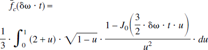
where ρ is the spin density, λ is the volume fraction of the cylinders, J₀(x) is the zeroth order Bessel function, and δω is the characteristic frequency that corresponds to the nuclear precession frequency in the equatorial field. In addition to the assumption of a random orientation for the cylinders, two major assumptions are made for this signal model. First, signal loss resulting from diffusion effects is ignored. Second, the signal loss induced by the paramagnetic particles within the cylinders is also neglected. The implications of these assumptions in the estimates of quantitative blood oxygen saturation in vivo are addressed in detail in the Discussion.

In the case of brain parenchyma, capillary vessels form a complicated interconnecting network of long cylinders, compared with their radii, with random orientations. Therefore, the theoretical model proposed by Yablonskiy and Haacke (1994) for a set of randomly orientated cylinders could be used to characterize the signal loss induced by the deoxyhemoglobin, the paramagnetic particles, outside of the intravascular space. If one assumes that the arterial blood is fully oxygenated then λ represents the venous blood volume and δω is the deoxyhemoglobin induced frequency shift which is defined as (Yablonskiy and Haacke, 1994)

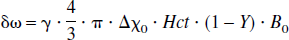
δ ω = γ \cdot \frac{4}{3} \cdot π \cdot Δ χ_{0} \cdot H c t \cdot (1 - Y) \cdot B_{0}

(3)

where γ is the gyromagnetic ratio, which is equal to 2.68 × 10⁸ rad/s/Tesla, Hct is the fractional hematocrit, B₀ is the main magnetic field strength, Y is the fractional cerebral blood oxygen saturation, and Δχ₀ is the susceptibility difference between fully oxygenated and fully deoxygenated blood that has been measured to be 0.18 ppm per unit Hct (Weisskoff and Kühne, 1992). To obtain a quantitative measurement of Y, δω must be extracted from Eq. 1. Unfortunately, Eq. 1 can not be solved analytically. Two asymptotic forms, namely a short time scale and a long time scale expression, are used to approximate Eq. 1 (Yablonskiy and Haacke, 1994).

For the short time scale, where δω · |t| ≤ 1.5, the asymptotic form can be written as

{\overset{ˉ}{S}}_{s} (t) = ρ \cdot (1 - λ) \cdot \exp [- 0.3 \cdot λ \cdot (δ ω \cdot t)^{2}] .

(4)

The subscript s denotes the short time scale. In contrast, for the long time scale, where δω · |t| > 1.5, the MR signal can be approximated by the following asymptotic form

{\overset{ˉ}{S}}_{l} (t) = ρ \cdot (1 - λ) \cdot \exp [- R 2^{'} \cdot (| t | - t_{c})] .

(5)

where the subscript l denotes the long time scale and t_c, the critical time, is defined as t₀=1/δω. Here R2′(= R*₂ – R₂, where R*₂ = 1/T*₂ and R₂ = 1/T₂) is the relaxation rate that characterizes the signal loss caused by local susceptibilities and can be written as

R 2^{'} = λ \cdot δ ω

(6)

Therefore, when R2′ and λ are known, an estimate of δω can be obtained from Eq. 6 that, in turn, provides a quantitative measurement of Y through Eq. 3.

MATERIALS AND METHODS

Magnetic resonance imaging experiments

Magnetic resonance imaging protocols were approved by the Human Study Committee at Washington University. In total, 8 normal healthy volunteer subjects were studied and written informed consent was obtained from all subjects.

All images were acquired on a Siemens 1.5T Symphony whole-body scanner (Siemens Medical Systems, Erlangen, Germany) with a gradient strength of 22 mT/m. A four-channel head array coil was used to receive the signal, whereas the body coil was used for transmitting. A two-dimensional, multi-echo gradient and spin echo sequence (Fig. 1) was used to acquire images and subsequently used to extract R2, R2′, and λ. In total, 21 echoes with an echo spacing of 4.96 milliseconds were acquired. The spin echo occurred at the eleventh echo and 10 echoes were placed symmetrically on each side of the spin echo. The echo times ranged from 63.18 milliseconds to 162.38 milliseconds with the spin echo occurring at 112.78 milliseconds. The imaging parameters were as follows: TR = 1000 milliseconds; field-of-view = 160 × 256 mm²; a matrix size of 160 × 256 resulting in an inplane resolution of 1 × 1 mm²; slice thickness = 7.5 mm; and two acquisitions to improve the signal-to-noise ratio. Although multislice acquisition could be achieved with the proposed method, only one slice was acquired in this study so that the potential crosstalk, signal interference between two adjacent slices because of an imperfect rf slice profile, could be minimized.

FIG. 1.

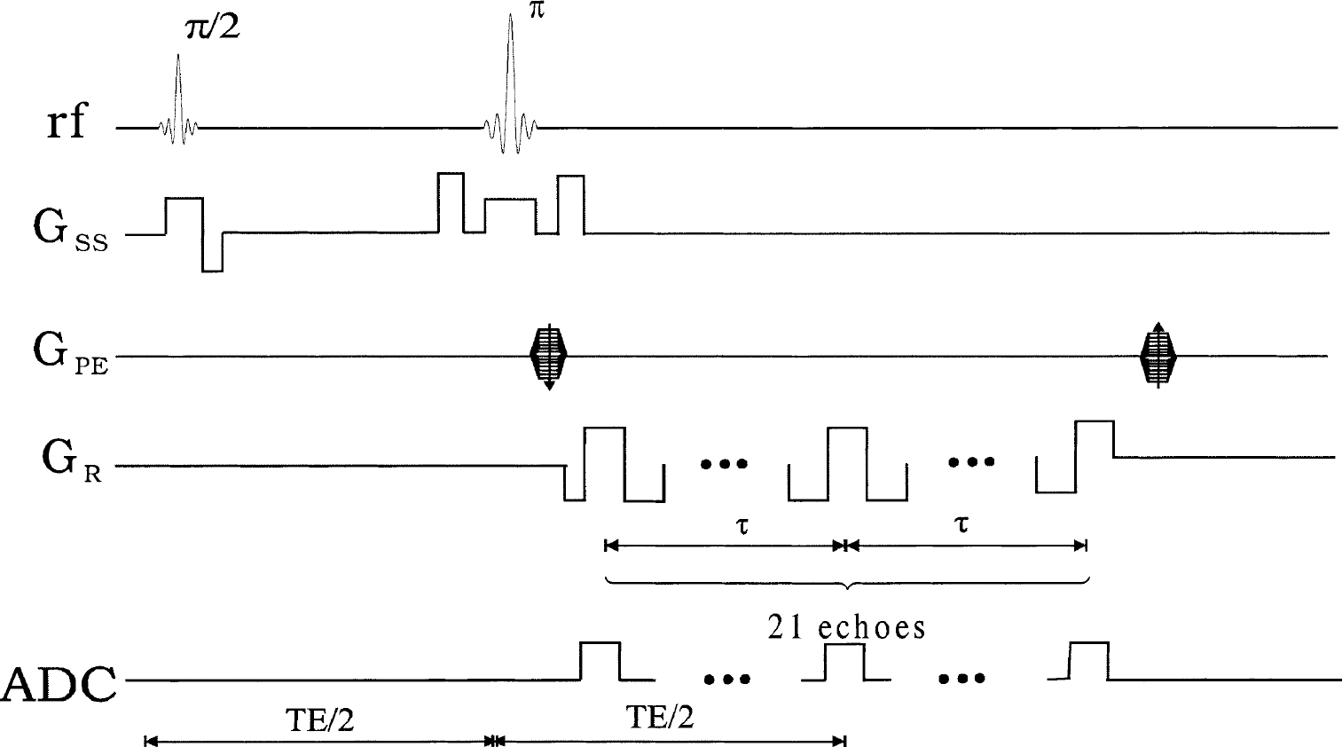
Sequence diagram of the multi-echo gradient and spin echo. G_ss, G_PE, and G_R represent the slice select, phase encoding, and frequency encoding, respectively. Analog-to-digital converter (ADC) indicates where images are acquired.

Estimations of R2, R2′, λ, and Y

All images were transferred to a Sun Workstation for postprocessing. To improve the signal-to-noise ratio, images were first collapsed to a matrix size of 128 × 128 before any postprocessing. Subsequently, R2 was extracted using

R 2 = \ln (\frac{S (T E - τ)}{S (T E + τ)}) / 2 τ

(7)

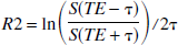
where TE is the echo time for the spin echo and τ is the time interval between the spin echo and the acquired gradient echoes (Fig. 1). By so doing, it is possible to obtain R2 estimates without worrying about the potential confounding factors associated with the differences in rf slice profiles between the 90° and 180° pulses (Yablonskiy and Haacke, 1997). To improve the accuracy of the R2 estimates, instead of relying on one pair of gradient echo images symmetrically placed about the spin echo, five pairs of gradient echo images (the 1–5th and the 17–21th gradient echoes) were used (Fig. 3A, unfilled squares) for the estimates of R2. Although it is possible to use more than five pairs of gradient echo images, the accuracy of the R2 estimates for the tissues of interest, such as gray matter and white matter, could be compromised if those with too short of a τ are included. A more detailed discussion for the choice of five gradient echo pairs is given in the Appendix.

FIG. 3.

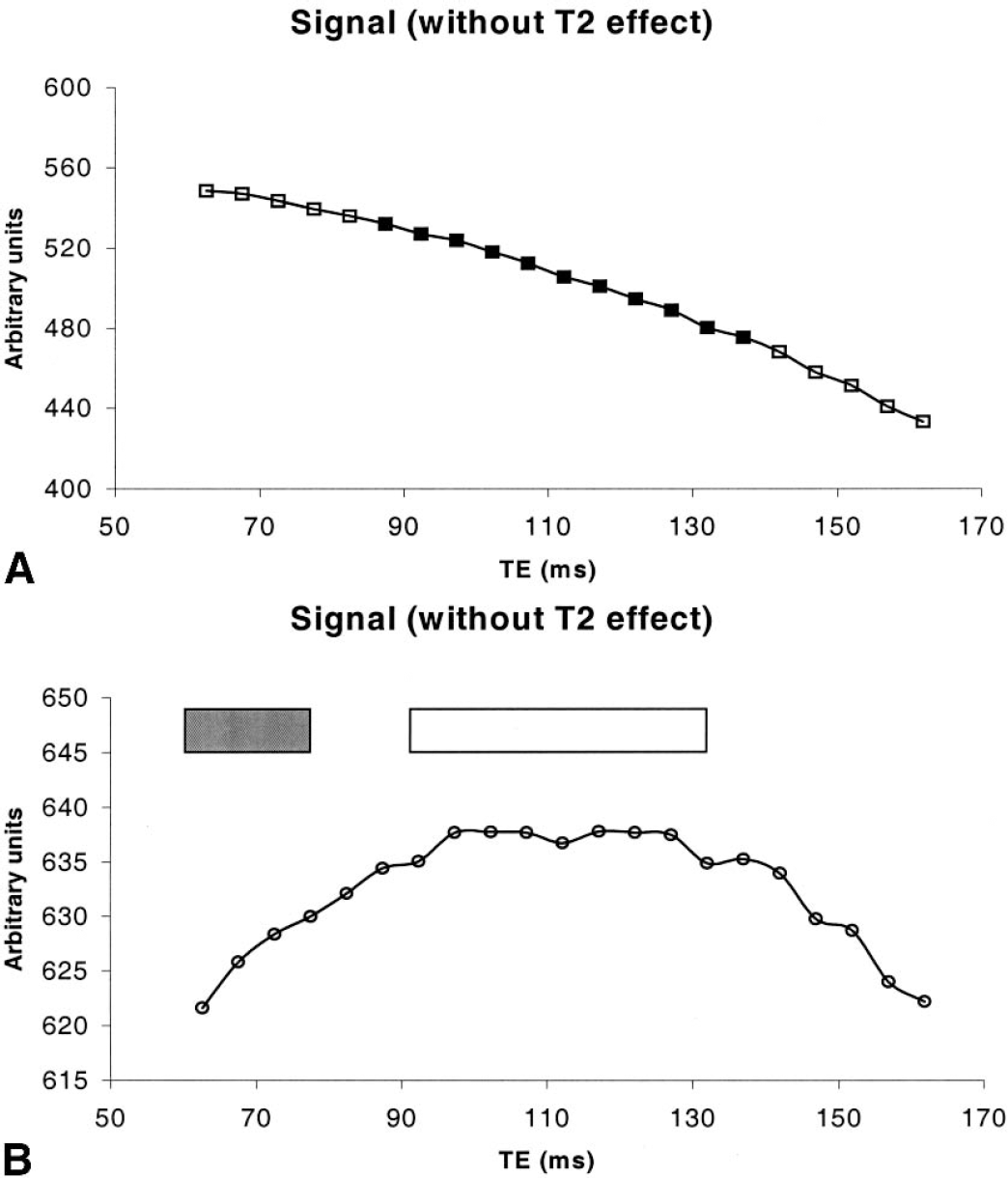
Experimentally measured signal is plotted as a function of TE (A) and the measured magnetic resonance signal after removing the R2 effect (B). Unfilled squares indicate the echoes used for the R2 estimates. In contrast, the filled box indicates the echoes used for the R2′ estimates, whereas the unfilled box represents the echoes used to fit a second order polynomial function.

After R2 was obtained, the effect of R2 was removed from the original signal so that Eqs. 4 and 5 could be used to describe the MR signal behavior in the presence of local magnetic field inhomogeneities. To better describe how R2′ and λ were estimated from the acquired images by the multi-echo gradient and spin echo sequence (Fig. 1), the t in Eqs. 4 and 5 was replaced by ΔTEi, which represents the time interval between the echo time of the i^th gradient echo and the echo time of the spin echo was 1 ≤ i ≤ 21.

By taking the natural logarithm of both sides of Eqs. 4 and 5, the authors found

\ln ({\overset{ˉ}{S}}_{s} (Δ T E_{i})) = a + [- 0.3 \cdot λ \cdot (δ ω \cdot Δ T E_{i})^{2}]

(8)

\ln ({\overset{ˉ}{S}}_{l} (Δ T E_{i})) = a + [- R 2_{c}^{'} \cdot (| Δ T E_{i} | - t_{c})] = - R 2_{c}^{'} \cdot | Δ T E_{i} | + b

(9)

where a = ln(ρ(1 – λ)) and b = a + R2′t_c. Notice that $\ln (({\overset{ˉ}{S}}_{s} (Δ T E_{i}))$ has a quadratic dependence on ΔTEi, while $\ln (({\overset{ˉ}{S}}_{l} (Δ T E_{i}))$ is linearly dependent on ΔTEi with a slope equal to R2′. Therefore, R2′ can be obtained with a linear least squares curve fitting of the MR signal of the gradient echoes as long as δω · |ΔTE_i| is greater than 1.5. In contrast, the signal from the central 9 echoes including the spin echo and 4 gradient echoes on each side of the spin echo (7^th – 15^th echoes, the unfilled box in Fig. 3B) was fitted to a second order polynomial function. This was done to minimize the effects of noise in the estimate of MR signal at the spin echo S_s(ΔTE = 0)) so that a more accurate estimate of λ could be obtained through the following equation (Yablonskiy, 1998).

λ = \ln ({\overset{ˉ}{S}}_{l} (Δ T E = 0) / {\overset{ˉ}{S}}_{s} (Δ T E = 0)) .

(10)

After obtaining R2′ and λ, δω can then be estimated from Eq. 6 and, finally, an absolute estimate of Y can be obtained through Eq. 3. In this study, a constant Hct of 0.42 was used for all subjects and a small vessel Hct to large vessel Hct ratio of 0.85 (Eichling et al., 1975) was used to convert the large vessel Hct to small vessel Hct.

Region of interest analysis

To obtain an estimate of R2, R2′, and λ in the brain parenchyma, an ROI that encompassed both hemispheres was used. However, six ROIs that equally divided each hemisphere into three ROIs were defined for the measurements of cerebral blood oxygen saturation of each volunteer. Both mean and standard deviation of R2, R2′, λ, and Y were recorded so that a comparison between subjects could be made.

Error analysis

An error analysis was performed to investigate how the presence of noise in the experimentally acquired MR images propagated through R2, R2′ and λ estimations to the final Y maps. Detailed descriptions of the error analysis for all estimated parameters including R2, R2′, λ, and Y are given in the Appendix.

RESULTS

Representative images obtained from the proposed sequence (Fig. 1), including the first echo (Fig. 2A), the 11^th echo (spin echo, Fig. 2B), and the last echo (Fig. 2C) from one subject are shown in Fig. 2. Although the first and the last echoes have exactly the same R2′ effects, a substantial decrease in signal-to-noise ratio is observed for the last echo when compared with the first echo. This is not surprising because the last echo has a larger T2 effect, leading to a reduction in MR signal, which in turn, decreases signal-to-noise ratio. In addition, the time interval between the first echo (last echo) and the spin echo is 49.6 milliseconds for the multi-echo gradient and spin sequence, which is analogous to a gradient echo sequence with a TE of 49.6 milliseconds. As a result, tissues with short T2*, such as subcutaneous fat, will not be visible in the first and the last gradient echo images. In contrast, the signal of subcutaneous fat (arrow) is recovered in the spin echo image because of the signal refocusing achieved by the 180° pulse.

FIG. 2.

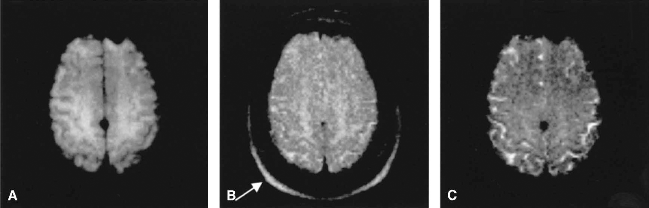
Anatomic images from the first echo (A), spin echo (B) and the last echo (C) obtained from the multi-echo gradient and spin echo sequence are shown.

Magnetic resonance signal as a function of TE is shown in Fig. 3A from a 4 × 4 region of one subject. The 21 points correspond to the signal from the 21 echoes acquired. Although the MR signal is anticipated to decay exponentially with two time constants, T₂ and T_2′, it is not immediately apparent owing to the fact that T_2′ is expected to be small and T2 will dominate the signal decay. After removing the effects of T2, the MR signal as a function of echo time is shown in Fig. 3B. As anticipated, the signal curve is symmetrical about the spin echo with the highest signal observed around the spin echo. The changes of MR signal are minimal when ΔTE is small, whereas a more rapidly decaying signal is observed for larger ΔTE. This is in agreement with theoretical expectations as described by Eqs. 4 and 5.

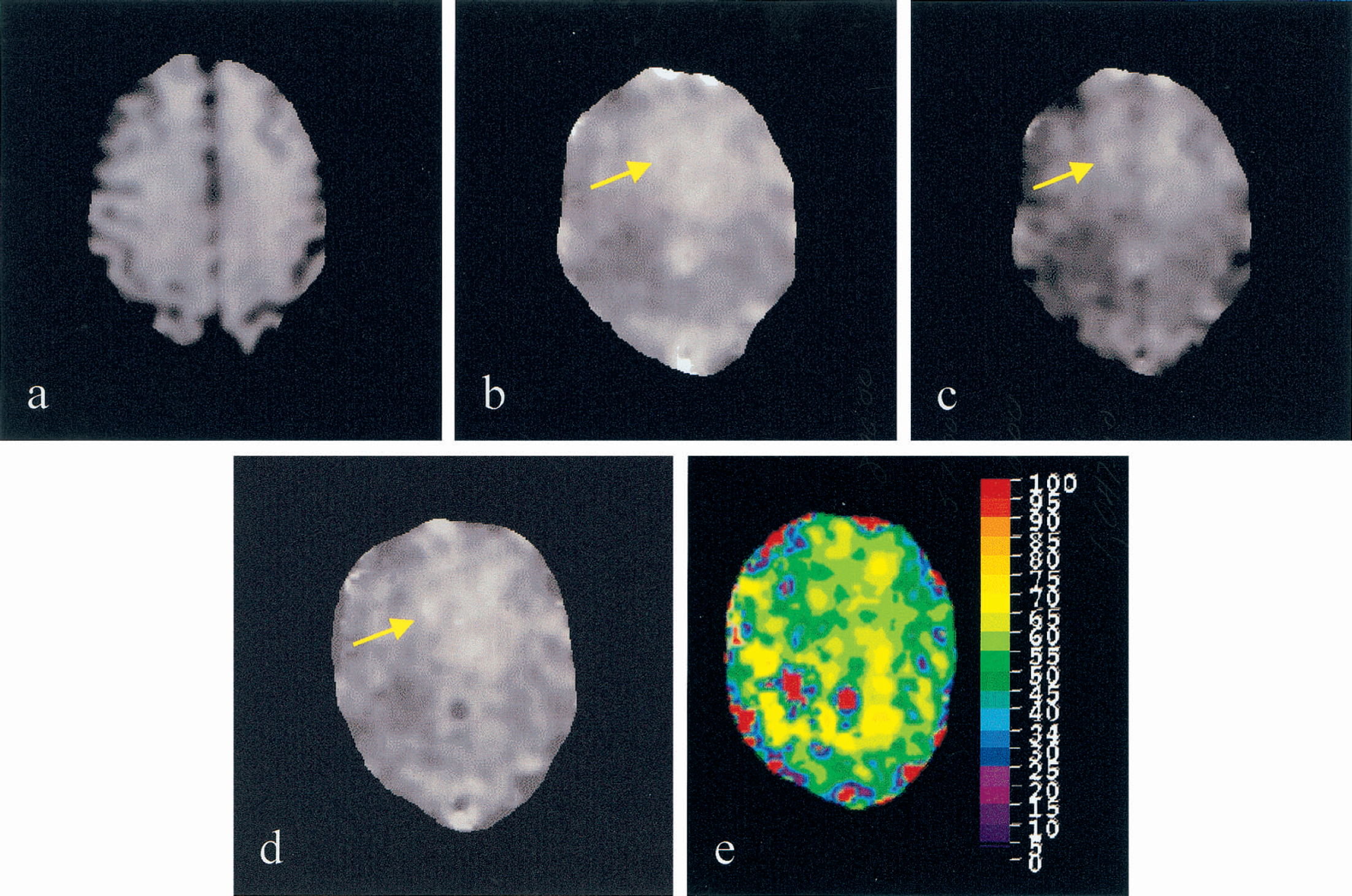
The estimated R2 (Fig. 4A), R2* (Fig. 4B), R2′ (Fig. 4C), blood volume fraction (Fig. 4D), and Y (Fig. 4E) maps from subject 8 are shown in Fig. 4 through the parameter estimation approach outlined in Materials and Methods. As anticipated, the CSF has a lower R2 when compared to the brain parenchyma and a rather uniform R2 map is observed for the brain parenchyma. In contrast, a slightly elevated R2* (arrow), R2′ (arrow) and blood volume fraction (arrow) is observed at the frontal area when compared with other regions of the brain parenchyma. Finally, although some spatial variations are also observed in the Y map (Fig. 4E), a rather uniform cerebral blood oxygen saturation ranging between 55.7% to 57.9% (Table 1, subject 8) in the brain parenchyma is obtained. Regions marked as red represent where the parameter estimations failed to estimate Y. The reasons for this are addressed in the Discussion.

FIG. 4.

R2 (A), R2* (B), R2′ (C), volume fraction (D), and color coded oxygen saturation Y (E) are shown. Color bar indicates the corresponding oxygen saturation from 0% to 100%.

TABLE 1.

Cerebral blood oxygen saturation measurements from volunteer studies

	Y (%)
Subject	1	2	3	4	5	6	7	8
Region 1	58.2 ± 7.3	58.7 ± 9.3	60.2 ± 5.4	55.6 ± 5.9	59.7 ± 7.9	59.9 ± 3.6	54.1 ± 4.9	55.7 ± 4.9
Region 2	57.5 ± 4.5	58.6 ± 5.0	58.8 ± 4.7	59.1 ± 11.2	65.2 ± 8.4	60.1 ± 4.3	52.2 ± 7.1	57.9 ± 7.2
Region 3	58.1 ± 3.7	56.5 ± 3.7	60.9 ± 7.4	55.1 ± 12.9	58.8 ± 6.5	61.2 ± 5.0	57.2 ± 8.1	57.2 ± 9.1
Region 4	55.5 ± 4.8	65.5 ± 8.8	58.1 ± 4.3	56.6 ± 5.2	55.3 ± 4.5	63.4 ± 3.7	55.1 ± 4.6	57.0 ± 5.2
Region 5	55.7 ± 5.3	61.1 ± 5.2	56.7 ± 4.3	62.8 ± 8.9	59.4 ± 5.8	63.5 ± 6.4	58.8 ± 7.4	57.3 ± 8.6
Region 6	57.1 ± 3.6	56.0 ± 4.0	53.7 ± 8.1	67.9 ± 9.3	57.6 ± 5.9	61.7 ± 2.8	54.1 ± 6.7	56.5 ± 7.3
Mean ± SD	57.5 ± 3.6	59.4 ± 6.4	58.1 ± 5.9	59.5 ± 9.3	59.3 ± 6.6	61.6 ± 4.5	55.3 ± 6.6	56.9 ± 7.2

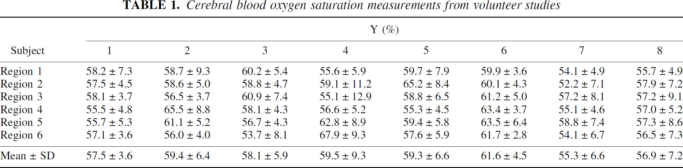
The measured R2, R2′, and λ in the brain parenchyma from all subjects are as follows: R2 = 10.5 ± 1.69 Hz; R2′ = 6.7 ± 3.92 Hz; and λ = 16.1 ± 7.43%. In addition, a summary of the estimated Y values from all volunteers is shown in Table 1 for all six regions, respectively. The estimated Y ranges between 55.3% to 61.6% in all subjects with a group mean of 58.4% ± 1.8%.

Finally, to investigate whether the observed spatial variation in the Y is caused by the noise in the acquired images or is indicative of physiologic variations, the calculated error of Y based on an error propagation analysis (Appendix) is compared with the experimentally measured intersubject variability shown in Table 1. An overall intersubject variability of 6.6% was obtained from the Y maps of all subjects. In contrast, an error of 5.24% is anticipated based on the error analysis (Eq. A12). Because the experimentally measured intersubject variability is only slightly higher than that obtained from the error analysis, the current results suggested that the observed spatial variation in the Y maps is likely to be dominated by noise with relatively little effects from physiologic variation.

DISCUSSION

It is well established that the brain extracts roughly 40% to 50% of available oxygen from the arterial blood to maintain neuronal activities under normal physiologic conditions in humans. With PET and continuous inhalation of ¹⁵O₂, Yamauchi et al. (1996) studied 10 normal volunteer subjects and an oxygen extraction fraction (OEF) of 42.6 ± 5.1% was obtained from different cortical areas. In addition, similar results were reported by Nakane et al. (1998) with continuous infusion of H₂¹⁵O. In total, 9 patients who exhibited no neurologic deficits and no apparent lesions on computed tomography were investigated. They showed that the OEF ranged between 40% to 44% in different cortical areas. To compare our estimates of cerebral blood oxygen saturation (Y) with those reported OEF values through PET measurements, it is necessary to convert the normal OEF values to the cerebral blood oxygen saturation.

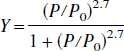
Under normal physiologic conditions, arterial blood can be assumed to be fully saturated (100%) with an oxygen content, Ca02, on the order of 19.2 vol % (Cooney, 1976). Assuming that the normal OEF is 42.6% based on the results obtained from Yamauchi et al. (1996), the Cvo2 can be calculated through the relation of OEF = (CaO2-Cvo2)/CaO2 that yields a Cvo2 of 10.9 vol %. Subsequently, the Cvo2 can be converted to oxygen saturation via the oxygen dissociation curve and the Hill equation (Cooney, 1976) through

Y = \frac{(P / P_{0})^{2.7}}{1 + (P / P_{0})^{2.7}}

where P is the partial pressure of oxygen and P₀ is the partial pressure for 50% saturation that is 27.2 mm Hg for PO2 = 95 mm Hg, PCO2 = 40 mm Hg, pH = 7.4 and a body temperature of 37°C. A cerebral blood oxygen saturation of 56.5% is therefore obtained based on the reported OEF in the literature. This is in excellent agreement with our results. A mean Y of 58.4% ± 1.8% was obtained from all subjects, implying that 41.6% ± 1.8% of available oxygen is extracted for maintaining normal neuronal activities from the arterial blood under normal physiologic conditions in humans. Our findings are encouraging and demonstrate the feasibility of using an MR imaging approach to obtain an estimate of in vivo cerebral blood oxygen saturation noninvasively.

However, the observed large intersubject variability in the estimates of Y from all subjects deserves further comment. As shown in Results, the experimentally measured intersubject variability (6.6%) is slightly higher than that obtained from the error analysis (5.24%). This suggests that the observed Y variations in the brain parenchyma are predominately derived from the presence of noise in MR images rather than physiologic variation. This is perhaps not surprising because a balance between cerebral blood flow and oxygen metabolism is normally preserved under normal physiologic conditions. The ratio of the two parameters (or OEF) has shown relatively little regional variation in the brain (Derdeyn and Powers, 1997). Our results are in agreement with those obtained from PET. However, given the large anticipated errors in our Y estimates, it is necessary to further improve the signal-to-noise ratios of the acquired images before the application of the proposed method in a clinical setting.

Model assumptions

Several assumptions are made for the signal model proposed by Yablonskiy and Haacke (1994) and three of them are particularly relevant to our study. The potential implications of the three assumptions on the measurements of Y are addressed below. First, the blood vessels are assumed to have a random orientation with respect to the static magnetic field so that a statistical approach can be used to derive the signal equation (Eq. 1). This was justified because the main thrust of our study was to obtain a quantitative measurement of cerebral blood oxygen saturation in the brain parenchyma. Given the large voxel size of 2 × 2 × 7.5 mm³ (after filtering the images to a matrix size of 128 × 128) and the fact that capillaries are very small in size (~10 μm) and randomly distributed in the brain parenchyma, this assumption should be fulfilled. However, it is not applicable to large vessels, such as pial veins, which could potentially occupy a substantial fraction of one voxel. This may explain some of the regions that are marked in red in Fig. 4E, in which the presence of large vessels is anticipated. As a result, the employed signal model fails to provide an estimate of Y in these voxels.

Second, only signal loss induced by the paramagnetic particles, deoxyhemoglobin, and outside of the cylinders is considered in this signal model. No intravascular effects are considered. This assumption could potentially impact on the estimates of Y under pathophysiologic conditions in which an elevated rCBV is anticipated (perhaps in regions of high grade tumors; Aroner et al., 1994) or if a voxel consists largely of blood. Functional MRI study is a typical example of the latter scenario in which the signal changes during a task-driven functional MRI study are primarily contributed by signal within the intravascular space of pial veins at a 1.5T system (Haacke et al., 1994; Boxerman et al., 1995; Song et al., 1996). Therefore, the proposed method may not be suitable for functional MRI studies without the appropriate modifications necessary to take into account the signal contribution in the intravascular space.

Nevertheless, normal volunteer subjects under a resting condition were studied. In addition, it is well known that normal cerebral blood volume ranges between 2% to 5% in the brain parenchyma (Grubb et al., 1973; Sakai et al., 1985; Perlmutter et al., 1987; Brooks et al., 1985; Leggett and Williams, 1991; Lin et al., 1997). Accordingly, the effects from large vessels, which do not form a random orientation or contribute largely to the signal in one voxel, are likely to be associated with specific anatomical locations and have minimal effects on the estimates of Y in the brain parenchyma. In addition, only images from the odd echoes (Fig. 1) were acquired and used for the estimates of Y. It is likely to further reduce the signal contributions from the flowing spins in the intravascular space because they will not be completely refocused by the odd echoes, resulting in a reduction in signal for the flowing spins.

Finally, signal dephasing induced by proton diffusion was also ignored in the signal model. To better address the effects of proton diffusion in the estimates of Y, the effects of diffusion in the intravascular space and extravascular space were considered separately. With a theoretical signal model, Kennan et al. (1994) have shown that the effects of diffusion in the intravascular space are both sequence and perturber size dependent. Based on simulation, they demonstrate that the effects of diffusion on MR signal are maximal when the size of the perturbers is on the order of 10μm, roughly the size of a capillary, for a spin echo sequence. Therefore, without taking into account the effects of diffusion in the intravascular space, errors in the Y estimates could occur. However, to what extent diffusion affects the Y estimates is weighted by the rCBV. Therefore, analogous to the previously arguments, the effects of diffusion in the intravascular space should be negligible owing to the rather small rCBV in the brain parenchyma.

In contrast, Kiselev and Posse (1999) have recently proposed an analytical model that appropriately takes into account the effects of diffusion in the extravascular compartment. With a computer simulation, their results suggest that the additional signal dephasing induced by diffusion in the extravascular space will cause the spin echo to occur earlier than expected, resulting in inaccurate measures of R2 with the proposed approach (Eq. 7) in our study. Subsequently, an overestimation of blood volume fraction was expected, leading to an underestimation of Y. To minimize the effects of diffusion in the extravascular space, a second order polynomial function was used to fit the signal around the spin echo including the spin echo (unfilled box in Fig. 3B). By so doing, the effects of diffusion were likely to be reduced and a more accurate estimate of the signal of the spin echo could be obtained.

Effects of sequence timing

As mentioned in the Theory section, the signal model proposed by Yablonskiy and Haacke (1994) can not be solved analytically, and two asymptotic forms were used to approximate the solutions. The limit to separate the two asymptotic forms is the product of δω and |ΔTE_i|. When δω*|ΔTE_i| is less than 1.5, the MR signal without R2 effects can be approximated by the short time scale expression, whereas the long time scale expression needs to be used when δω*|ΔTE_i| is greater than 1.5. The latter requirement is particularly important for obtaining an accurate estimate of R2′ because a linear least squares curve fitting is used to fit the acquired MR signal and the slope of this fitted line provides an estimate of R2′. To ensure that the MR signal used for the curve fitting meets the requirement, a priori knowledge of δω is needed, which in turn, requires a known Y. Obviously, Y is the parameter that will be estimated and yet it is unknown before the MR imaging experiments. Therefore, it is of importance to determine the upper limit of the oxygen saturation that can be accurately estimated with the used sequence timing of the multi-echo gradient and spin echo sequence in our study.

Four MR images acquired with a ΔTE_i of 34.72 milliseconds, 39.68 milliseconds, 44.64 milliseconds, and 49.6 milliseconds (filled box in Fig. 3B) were used for the linear curve fitting to obtain an estimate of R2′. Under this condition, the product of δω*|ΔTE_i| will always be greater than 1.5 for all four images when Y is less than 60%. It fulfills the requirement for the utilization of the long time scale expression to obtain an estimate of R2′, which in turn, allows us to obtain an accurate estimate of Y. Conversely, when Y is greater than 60%, some of the four images used for the linear curve fitting will lie within the short time scale regime leading to inaccuracy in the estimates of R2′. This is because the signal within the short time scale regime will no longer be linearly dependent on ΔTEi, but rather quadratically dependent on ΔTEi. As a result, an underestimation of Y can occur when Y is greater than 60%. The degree of underestimation in Y is highly dependent on the true Y values, with larger underestimation for higher Y. Although a quantitative estimate of the degree of underestimation for Y values greater than 60% can be obtained with a Monte Carlo simulation, it was not done because a cerebral blood oxygen saturation of 56.5% was reported from normal volunteer subjects (Yamauchi et al., 1996). Therefore, the employed sequence timing should allow us to obtain an accurate estimate of Y in normal volunteers. However, modifications by increasing ΔTEi will be needed when cerebral blood oxygen saturation greater than 60% is anticipated such as under hyperemic or hypercapnic conditions. Further studies will be needed to assess the accuracy of the proposed methods in obtaining quantitative estimates of Y under these pathophysiologic conditions.

Effects of other paramagnetic sources and magnetic field variations

It has been demonstrated by many investigators with MR and PET that the total cerebral blood volume including arterial and venous blood pools is approximately 2% to 3% and 4% to 5% for the white matter and gray matter, respectively (Grubb et al., 1973; Sakai et al., 1985; Perlmutter et al., 1987; Brooks et al., 1985; Leggett and Williams, 1991, Kuppusamy, 1996). Although a wide range of the ratio of cerebral venous blood volume to the total cerebral blood volume has been reported (0.75 to 0.85) in the literature (Tomita et al., 1978; Tomita, 1988), (Pollard et al. 1996a,b) recently demonstrated that a ratio of 0.75 would be a reasonable choice under normal physiologic conditions. Thus, a venous blood volume fraction of 1.5% to 2.3% and 3% to 3.8% is anticipated for white matter and gray matter, respectively.

However, a λ = 16.1 ± 7.43% was obtained from all subjects in our study. This is clearly much higher than the reported venous blood volume fraction. In addition, an elevated R2′ and λ in the frontal areas where air—tissue interface effects are present is also observed in some volunteer subjects. These observed elevations of R2′ and λ are likely because paramagnetic sources other than deoxyhemoglobin are present in vivo and can induce an additional signal loss in the MR images. These sources include other paramagnetic particles and magnetic field variations. The former case contains, for example, blood products and calcified plaques. Because normal volunteer subjects were studied, it is unlikely that these paramagnetic sources existed. In contrast, the latter case could potentially affect our estimates of Y. There are two potential situations in which magnetic field variations can be present: the local susceptibility differences between tissues, such as air—tissue interfaces, and a nonuniform static magnetic field across the slice thickness. In both cases, the additional signal decay can be characterized by an additional sinc function multiplied into Eq. 1 (Hardy et al., 1990), leading to a more rapid signal decay when compared with the condition in which deoxyhemoglobin is the only paramagnetic source. As a result, an overestimation of R2′ is anticipated. In addition, because the effects of magnetic field variation will be completely eliminated by the application of a 180° refocusing pulse, the signal in a spin echo image remain unaffected. Consequently, an overestimation of λ is also anticipated. This is due to the fact that the numerator in Eq. 10 is increased because of increased R2′, Eq. 9, whereas the denominator will remain unchanged. As a result, an overestimation of R2′ and λ is likely to be present in our results.

Because the main thrust of this study was to obtain a quantitative estimate of in vivo blood oxygen saturation, the observed overestimation of R2′ and λ needs to be discussed in the context of Y. As shown in Eq. 6, δω, and thus Y, is obtained by taking the ratio of R2′ and λ. With the additional signal loss induced by the presence of magnetic field variation, R2′ and λ were expected to be overestimated. If one can assume that the overestimated R2′ and λ are similar in magnitude to the first order, then the magnetic field variation will have minimal effects on Y. Based on the calculation of the correlation coefficient between R2′ and λ (Appendix, Eq. A13), it was found to be 0.94, indicating that the two parameters have a highly linear relation. This may explain the observed a rather uniform Y in the entire brain parenchyma in Fig. 4E despite the elevated R2′ and λ in the frontal regions where air—tissue interface is present. More importantly, a group mean of 58.4% ± 1.8% was obtained for the MR estimated Y from all volunteers, comparing favorably with that reported in the literature. Nonetheless, to obtain a more accurate estimate of Y and λ, local magnetic field variations will need to be taken into account. Several different approaches to minimize the effects of magnetic field variations are currently under investigation and it is beyond the scope of the current study.

Ratio of small vessel to large vessel Hct

To obtain a quantitative measurement of cerebral blood oxygen saturation, a known Hct is required (Eq. 3). Although it is possible to obtain a direct measurement of the large vessel Hct from each volunteer, it is not done because the large vessel Hct has been known to be rather stable in humans. It ranges between 0.4–0.45 depending on the gender (Braunwald et al., 1987). Therefore, a constant large vessel Hct of 0.42 was assumed in this study for all volunteer subjects. However, this large vessel Hct needs to be converted to the small vessel Hct before the estimation of Y through Eq. 3. A wide range of the ratio of small vessel cerebral Hct (cHct) to large vessel Hct (cHct/Hct = 0.62–0.92) has been reported by different investigators in different species including humans (Cremer and Seville, 1983; Everett et al., 1956; Levin and Ausman, 1969; Larsen and Lassen, 1964; Oldendorf et al., 1965). Despite these discrepancies in the reported cHct/Hct ratios, a general consensus of cHct/Hct = 0.85 has been used by PET (Eichling et al., 1975). Therefore, a cHct/Hct of 0.85 was used in the current study to convert the large vessel Hct to cHct.

With a constant Hct used in the current study, errors may have occurred because of the potential variation in Hct between subjects and the uncertainty in cHct/Hct ratio. Specifically, as shown in Eq. 3, δω is directly proportional to Hct. Consequently, errors induced by the inaccuracy in Hct will contribute directly to the estimates of Y. Nevertheless, the errors induced by the former case are a global effect and may be easily overcome with a direct measurement of Hct from each subject. Therefore, the potential variation in Hct between subjects should not affect the proposed method in obtaining a quantitative measurement of cerebral blood oxygen saturation. In contrast, the potential errors induced by the latter factor are likely to be small under normal physiologic conditions and are beyond the scope of this study.

In conclusion, because the discovery of BOLD contrast, MR has shown promise in obtaining quantitative estimates of blood oxygen saturation in vivo. However, technical difficulties in the estimates of parameters, such as R2′ and λ, have hampered the success in obtaining in vivo blood oxygen saturation. The goal of the current study was to demonstrate that an absolute estimate of blood oxygen saturation could be obtained noninvasively with an MR imaging approach. Despite the simplifications of the signal model for the capillary network in an organ as complex as the brain and some confounding factors that still needed to be resolved, a mean cerebral blood oxygen saturation of 58.4% ± 1.8% was obtained from all subjects. This is in excellent agreement with the known cerebral blood oxygen saturation under normal physiologic conditions. Although more systematic validations in animal models will be needed before the application of the proposed method in a clinical setup, our preliminary results are encouraging and underscore the possibility of using an MR imaging approach for obtaining an absolute estimate of cerebral blood oxygen saturation in vivo.

Footnotes

APPENDIX

Acknowledgment

The authors are grateful to Dr. E. Mark Haacke for his valuable input and participation in several discussions on the theoretical aspects of this work.

Abbreviations used

References

Aroner

Gazit

Louis

(1994) Cerebral blood volume maps of gliomas: comparison with tumor grade and histologic findings. Radiology 191:41–51

Boxerman

Hamberg

Rosen

Weiskoff

(1995) MR Contrast Due to Intravascular Magnetic Susceptibility Perturbations. Magn Reson Med 34:555–566

Braunwald

Isselbacher

Petersdorf

Wilson

Martin

Fauci

(1987) Harrison's principles of internal medicine. New York, NY: McGraw-Hill Book Company

Brooks

Beaney

Leenden

Marshall

Thomas

Jones

(1985) Regional cerebral oxygen utilization, blood flow and blood volume in benign intracranial hypertension studied by PET. Neurology 35:1030–1034

Bullock

Stewart

Rafferty

Teasdale

(1993) Continuous monitoring of jugular bulb oxygen saturation and the effect of drugs acting on cerebral metabolism. Acta Neurochir Suppl (Wein) 59:113–118

Cooney

(1976) Biomedical engineering principles: an introduction to fluid, heat, and mass transport processes. New York, NY: Marcel Dekker Inc. pp 356–362

Cremer

Seville

(1983) Regional brain blood flow, blood volume, and haematocrit values in the adult rat. J Cereb Blood Flow Metab 3:254–256

Cruz

Miner

Allen

Alves

Gennarelli

(1990) Continuous monitoring of cerebral oxygenation in acute brain injury: injection of mannitol during hyperventilation. J Neurosurg 73:725–730

Cruz

(1993) Jugular venous oximetry. Acta Neurochir Suppl (Wein) 59:86–90

10.

Cruz

(1988) Continuous versus serial global cerebral hemometabolic monitoring: applications in acute brain trauma. Acta Neurochir Suppl (Wein) 42:35–39

11.

De Crespigny

Wendland

Derugin

Kozniewska

Moseley

(1992) Real-time observation of transient focal ischemia and hyperemia in cat brain. Magn Reson Med 27:391–397

12.

Davis

Kwong

Weisskoff

Rosen

(1998) Calibrated functional MRI: mapping the dynamics of oxidative metabolism. Proc Natl Acad Sci U S A 95:1834–1839

13.

Derdeyn

Powers

(1997) Metabolic studies using PET in stroke investigation. In: Primer on cerebrovascular diseases ( Welch

KMA

Caplan

Reis

Siesjo

Weir

, eds) San Diego, CA: Academic Press, pp 644–650

14.

Eichling

Raichle

Grubb

Larson

Ter-Pogossian

(1975) In vivo determination of cerebral blood volume with radioactive oxygen-15 in the monkey. Circ Res 37:707–714

15.

Everett

Simmons

Lasher

(1956) Distribution of blood (Fe⁵⁹) and plasma (I¹³¹) volumes of rats determined by liquid nitrogen freezing. Circ Res 4:419–424

16.

Foltz

Merchant

Downar

Stainsby

Wright

(1999) Coronary venous oximetry using mRI. Magn Reson Med 42:837–848

17.

Grotta

(1986) Emerging stroke therapies. Neurology 6(3):285–292

18.

Grubb

Phelps

Ter-Pogossian

(1973) Regional blood volume in humans: x-ray fluorescence studies. Arch Neurol 28:31–44

19.

Haacke

Brown

Thompson

Venkatesan

(1999) Magnetic resonance imaging—physical principles and sequence design. New York, NY: John Wiley and Sons

20.

Haacke

Hopkins

Lai

Buckley

Friedman

Meltzer

Hedera

Friedland

Klein

Thompson

(1994) 2D and 3D high resolution gradient echo functional imaging of the brain: venous contributions to signal in motor cortex studies. NMR Biomed 7:54–62

21.

Hardy

Kucharczyk

Henkelman

(1990) Cause of signal loss in MR images of old hemorrhagic lesions. Radiology 174:549–555

22.

Heiss

Rosner

(1983) Functional recovery of cortical neurons as related to degree and duration of ischemia. Ann Neurol 14:294–301

23.

Heiss

Graf

Wienhard

Lottgen

Saito

Fujita

Rosner

Wagner

(1994) Dynamic penumbra demonstrated by sequential multitracer PET after middle cerebral artery occlusion in cats. J Cereb Blood Flow 14:892–902

24.

Hoppel

Weisskoff

Thulborn

Moore

Kwong

Rosen

(1993) Measurement of regional blood oxygenation and cerebral hemodynamics. Magn Reson Med 30:715–723

25.

Jezzard

Heineman

Taylor

DesPres

Wen

Balaban

Turner

(1994) Comparison of EPI gradient-echo contrast changes in cat brain caused by respiratory challenges with direct simultaneous evaluation of cerebral oxygenation via a cranial window. NMR in Biomed 7:35–44

26.

Jones

Morawetz

Crowell

(1981) Thresholds of focal ischemia in awake monkeys. J Neurosurg 54:773–782

27.

Kennan

Zhong

Gore

(1994) Intravascular susceptibility contrast mechanism in tissues. Magn Reson Med 31:9–21

28.

Kennan

Scanley

Gore

(1997) Physiological basis for BOLD MR signal changes due to hypoxia/hyperoxia: separation of blood volume and magnetic susceptibility effects. Magn Reson Med 37:353–356

29.

Kiselev

Posse

(1999) Analytical model of susceptibility-induced MR signal dephasing: effect of diffusion in a microvascular network. Magn Reson Med 41:499–509

30.

Kuppusamy

Lin

Cizek

Haacke

(1996) A quantitative assessment of in vivo regional cerebral blood volume using high resolution 3D T1 weighted pre and post injection of a contrast agent. Radiology 201:106–112

31.

Larsen

Lassen

(1964) Cerebral hematocrit in normal man. J Appl Physiol 19:571–574

32.

Levin

Ausman

(1969) Relationship of peripheral venous hematocrit to brain hematocrit. J Appl Physiol 26:433–437

33.

Leggett

Williams

(1991) Suggested reference values for regional blood volumes in humans. Health Phys 60:139–154

34.

Lin

Paczynski

Kuppusamy

Hsu

Haacke

(1997) Quantitative measurements of regional cerebral blood volume using MRI in rats: effects of arterial carbon dioxide tension and mannitol. Magn Reson Med 38:420–428

35.

Lin

Paczynski

Celik

Kuppusamy

Hsu

Powers

(1998a) Experimental hypoxemic hypoxia: changes in R2* of brain parenchyma accurately reflect the combined effects of changes in arterial and cerebral venous oxygen saturation. Magn Reson Med 39:474–481

36.

Lin

Paczynski

Celik

Hsu

Powers

(1998b) Effects of acute normovolemic hemodilution on T2*-weighted images of rat brain. Magn Reson Med 40:857–864

37.

Lin

Celik

Paczynski

Hsu

Powers

(1999) Quantitative magnetic resonance imaging in experimental hypercapnia: improvement in the relation between changes in brain R2* and the oxygen saturation of venous blood after correction for changes in cerebral blood volume. J Cereb Blood Flow Metab 19:853–862

38.

Majumdar

(1991) Quantitative study of the susceptibility difference between trabecular bone and bone marrow: computer simulation. Magn Reson Med 22:101–110

39.

Majumdar

Thomasson

Shimakawa

Genant

(1991) Quantitation of the susceptibility difference between trabecular bone and bone marrow: experimental studies. Magn Reson Med 22:111–127

40.

Muller

Gillis

Moiny

Roch

(1991) Transverse relaxivity of particulate MRI contrast media: from theories to experiment. Magn Reson Med 22:178–182

41.

Nakane

Ibayashi

Fujil

Sadoshima

Irie

Kitazono

Fujishima

(1998) Cerebral blood flow and metabolism in patients with silent brain infarction: occult misery perfusion in the cerebral cortex. J Neurol Neurosurg Psychiatry 65:317–321

42.

Ogawa

Lee

(1990a) Magnetic resonance imaging of blood vessels at high field: in vivo and in vitro measurements and image simulation. Magn Reson Med 16:9–18

43.

Ogawa

Lee

Kay

Tank

(1990b) Brain magnetic resonance imaging with contrast dependent on blood oxygenation. Proc Natl Acad Sci U S A 87:9698–9872

44.

Ogawa

Lee

Nayak

Glynn

(1990c) Oxygenation-sensitive contrast in magnetic resonance image of rodent brain at high magnetic fields. Magn Reson Med 14:68–78

45.

Ogawa

Lee

Barrere

(1993a) The sensitivity of magnetic resonance image signals of a rat brain to changes in the cerebral venous blood oxygenation. Magn Reson Med 29:205–210

46.

Ogawa

Menon

Tank

Kim

Markle

Ellermann

Ugurbil

(1993b) Functional brain mapping by blood oxygenation level-dependent contrast magnetic resonance imaging. Biophysical J 64:803–812

47.

Oldendrof

Kitano

Shimizu

Oldendorf

(1965) Hematocrit of the human cranial blood pool. Circ Res 17:532–539

48.

Ono

Morikawa

Inubushi

Shimizu

Yoshimoto

(1997) T2*-weighted magnetic resonance imaging of cerebrovascular reactivity in rat reversible focal cerebral ischemia. Brain Res 744:207–215

49.

Perlmutter

Powers

Herscovitch

Fox

Raichle

(1987) Regional asymmetries of cerebral blood flow, blood volume, and oxygen utilization and extraction in normal volunteers. J Cereb Blood Flow Metab 7:64–67

50.

Plum

Pulsinelli

(1986) Cerebral metabolism and hypoxic-ischemic brain injury. In: Diseases of the central nervous system ( Asbury

McKhann

McDonald

, eds), Philadelphia: W. B. Saunders, pp 1086–1101

51.

Pollard

Prough

DeMelo

Deyo

Uchida

Stoddart

(1996a) Validation in volunteers of a near infrared spectroscope monitoring brain oxygenation in vivo. Anesth Analg 82(2):269–277

52.

Pollard

Prough

DeMelo

Deyo

Uchida

Widman

(1996b) The influence of carbon dioxide and body position on near-infrared spectroscopic assessment of cerebral hemoglobin oxygen saturation. Anesth Analg 82(2):278–287

53.

Press

Teukolsky

Vetterling

Flannery

(1992) Numerical recipes in C, the art of scientific computing. 2nd ed. Cambridge, England: Cambridge University Press

54.

Prielmeier

Nagatomo

Frahm

(1994) Cerebral blood oxygenation in rat brain during hypoxic hypoxia: quantitative MRI of effective transverse relaxation rates. Magn Reson Med 31:678–681

55.

Rostrup

Larsson

HBW

Toft

Garde

Henriksen

(1995) Signal changes in gradient echo images of human brain induced by hypo- and Hyperoxia. NMR in Biomed 8:41–47

56.

Sakai

Nakazawa

Tazaki

Ishii

Hino

Igarashi

Kanda

(1985) Regional cerebral blood volume and hematocrit measured in normal human volunteers by single photon emission computed tomography. J Cereb Blood Flow Metab 5:207–213

57.

Sharan

Jones

Koehler

Traystman

Popel

(1989) A compartmental model for oxygen transport in brain microcirculation. Ann Biomed Eng 17:13–38

58.

Siesjo

(1978) Brain energy metabolism. New York, NY: John Wiley and Sons

59.

Song

Wong

Tan

Hyde

(1996) Diffusion weighted fMRI at 1.5T. Magn Reson Med 35:155–158

60.

Stables

Kennan

Gore

(1998) Asymmetric spin-echo imaging of magnetically inhomogeneous system: theory, experiment, and numerical studies. Magn Reson Med 40:432–442

61.

Tomita

Gotoh

Aamano

Tanahashi

Kobari

Shinohara

Mihara

(1978) Transfer function through regional cerebral cortes evaluated by a photoelectric method. Am J Physiol 235:H56–63

62.

Tomita

(1988) Significance of cerebral blood volume. In: Cerebral hyperemia and ischemia: from the standpoint of cerebral blood volume ( Tomita

Sawada

Naritomi

Heiss

, eds), New York, NY: Elsevier Science, pp 3–30

63.

Turner

Le Bihan

Moonen

CTW

Despres

Frank

(1991) Echo-planar time course MRI of cat brain oxygenation changes. Magn Reson Med 22:159–166

64.

Van Zijl

Eleff

Ulatowski

Oja

Ulug

Traystman

Kauppinen

(1998) Quantitative assessment of blood flow, blood volume and blood oxygenation effects in functional magnetic resonance imaging. Nat Med 4(2):159–167

65.

Weisskoff

Kiihne

(1992) MRI susceptometry: image-based measurement of absolute susceptibility of MR contrast agents and human blood. Magn Reson Med 24:375–383

66.

Wright

Macovski

(1991) Estimation oxygen saturation of blood in vivo with MR imaging at 1.5T. J Magn Reson Imaging 1:275–283

67.

Yablonskiy

Haacke

(1994) Theory of NMR signal behavior in magnetically inhomogeneous tissues: the static dephasing regime. Magn Reson Med 32:749–763

68.

Yablonskiy

Haacke

(1997) An MRI method for measuring T2 in the presence of static and RF magnetic field inhomogeneities. Magn Reson Med 37(6):872–876

69.

Yablonskiy

(1998) Quantitation of intrinsic magnetic susceptibility-related effects in a tissue matrix. Phantom study. Magn Reson Med 39:417–428

70.

Yamauchi

Fukuyama

Nagahama

Nabatame

Nakamura

Yamamoto

Yonekura

Konishi

Kumura

(1996) Evidence of misery perfusion and risk for recurrent stroke in major cerebral arterial occlusive diseases from PET. J Neurol Neurosurg Psychiatry 61:18–25

Quantitative Measurements of Cerebral Blood Oxygen Saturation Using Magnetic Resonance Imaging

Abstract

Keywords

Theory

MATERIALS AND METHODS

Magnetic resonance imaging experiments

Estimations of R2, R2′, λ, and Y

Region of interest analysis

Error analysis

RESULTS

DISCUSSION

Model assumptions

Effects of sequence timing

Effects of other paramagnetic sources and magnetic field variations

Ratio of small vessel to large vessel Hct

Footnotes

APPENDIX

Acknowledgment

Abbreviations used

References