Sage Journals: Discover world-class research

Abstract

This article develops a theoretical framework for the use of the wavelet transform in the estimation of emission tomography images. The solution of the problem of estimation addresses the equivalent problems of optimal filtering, maximum compression, and statistical testing. In particular, new theory and algorithms are presented that allow current wavelet methodology to deal with the two main characteristics of nuclear medicine images: low signal-to-noise ratios and correlated noise. The technique is applied to synthetic images, phantom studies, and clinical images. Results show the ability of wavelets to model images and to estimate the signal generated by cameras of different resolutions in a wide variety of noise conditions. Moreover, the same methodology can be used for the multiscale analysis of statistical maps. The relationship of the wavelet approach to current hypothesis-testing methods is shown with an example and discussed. The wavelet transform is shown to be a valuable tool for the numerical treatment of images in nuclear medicine. It is envisaged that the methods described here may be a starting point for further developments in image reconstruction and image processing.

Keywords

Wavelets Estimation Positron emission tomography Single-photon emission computed tomography Compression Filtering

The wavelet transform (WT) is a mathematical tool that has been recently introduced for the analysis of nonstationary signals (Meyer, 1992; Daubechies, 1992). WT methods differ from traditional Fourier methods by their inherent ability of localizing information in the time-frequency domain. These methods have been extensively used in many areas of signal processing and they have been shown to be particularly suitable for application in the biomedical field (Unser and Aldroubi, 1996). The analysis of images obtained with positron emission tomography (PET) or single-photon emission computed tomography (SPECT) is one such application where WT may be used to detect signal of unknown position and scale in the data volume (Unser et al., 1995; Ruttiman et al., 1996). In this context, wavelet filters have been also applied to denoise time-activity curves (Millet et al., 1998).

This article builds on previous work to define a new theoretical framework and new fast algorithms for the statistical estimation of images obtained with emission tomography (ET), from either PET or SPECT scanners. The text is first intended to give a short overview of the current wavelet methodology. The second and main goal of the article is to devise a new wavelet methodology that deals with two relevant properties of ET images: correlated (colored) noise and low signal-to-noise ratio. Finally, the application of the new methods to simulated and real data-sets illustrates the use of such techniques and elucidates their properties and limitations.

THE PROBLEM OF ESTIMATION

We are interested in the analysis of images acquired with an ET, reconstructed from sinograms or planar projections at their highest resolution using back-projection with a ramp filter.

The problem of estimation of such an image may be defined in the usual framework of function estimation. We suppose we are given some noisy samples of a function F:

Y (t) = f (t) + e (t)

(1)

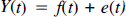
where t = 1,…., M, is one of the M sites where F is measured (i.e., a pixel in the case of an image) and e(t) are M independent normal random variables with mean 0 and unknown variance σ² (in notation: e(t) ∼ N(0, σ²)).

The problem of interest is the recovery of F(t) from the noisy data without assuming any particular parametric form for F with small mean-squared error or, more formally, the computation of an estimate depending on y₁,…., y_M with small risk 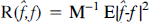, where E( ) is the expected value and the norm 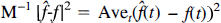is the usual L₂ -norm of least square estimation.

WAVELETS BASIS FUNCTIONS

There are several approaches to the nonparametric estimation of an unknown function F (Donoho and Johnstone, 1994). We are interested in transform methods that represent F as a finite sum of some suitable functions φ_ω(t) indexed by the parameter ω thus forming a functional base F = {φ_ω(t), ω ε R}. For instance, the Fourier transform (FT) expands the function F in the familiar set of periodic functions:

F_{F T} = {φ_{ω} (t) = e^{i ω t} = s i n (ω t) + i c o s (ω t), ω \in R},

(2)

where the parameter ω is termed frequency. By projecting the data into this functional space, FT methods estimate the function f in terms of its frequency components φ_ω(t). This is the frequency localization property of the FT; the obvious drawback is that in the frequency domain all the time information is lost. This lack of localization in time makes the FT unsuitable for non stationary signals, that is those signals characterized by local frequency changes.

To overcome this limitation, dyadic wavelet transform (DWT) methods use the functional base:

F_{WT} = {ψ_{j k} (t) = 2^{- j / 2} ψ (2^{- j} t - k), (j, k) \in Z^{2}},

(3)

that is obtained by translation and dilation of a single wavelet function Ψ(t). A number of suitable wavelet functions Ψ((t) have been found that are able to provide both time and frequency localization (Aldroubi, 1996). Figure 1 shows one of such wavelets and its properties in the time and frequency domains. The ideal system of finite (or compact) support both in time and frequency cannot be achieved as asserted by the theory of analytic functions (Bracewell, 1986). Therefore, the choice between a compact support in time or frequency depends on the type of application.

FIG. 1.

The Battle-Lemarie wavelet is a smooth, symmetric wavelet with compact support in the frequency space but also good localization properties in the time space. Figures show the scaling function and wavelet function with their correspondent Fourier transforms for the first resolution level (A) and second resolution level (B). Note that the spectra of the scaling and wavelet functions are complementary, as are the spectra of wavelet functions at different resolution levels.

WT shares some optimality properties with FT. The functional base F_FT is an unconditional base for all periodic functions; this means that F_FT is orthonormal and that any periodic function can be expressed by one and one only linear combination of the elements of F_FT (Donoho, 1996). Wavelet bases F_WT provide unconditional bases for a wide set of functional spaces such as Besov or Triebel spaces (Donoho, 1993; 1996). In practical terms, bases of smooth wavelets are the best bases for representing functions of bounded variation that may have jumps localized in one part of the domain and be very flat elsewhere. For instance, consider the Gaussian functions that are often used to model the signal in ET images (Worsley et al., 1996); these functions are examples of Bump Algebra that is a functional space in the Besov scale (Donoho and Johnstone, 1992).

DYADIC WAVELET TRANSFORM

DWT decomposes a signal into a set of orthogonal components describing the signal variation across scales (Mallat, 1989). In analogy with other function expansions, a function J may be written, for each discrete coordinate t, as a sum of a wavelet expansion up to a certain scale J plus a residual term, that is:

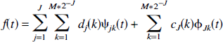
f (t) = \sum_{j = 1}^{J} \sum_{k = 1}^{M * 2^{- J}} d_{j} (k) ψ_{j k} (t) + \sum_{k = 1}^{M * 2^{- J}} c_{J} (k) ϕ_{J k} (t)

(4)

Equation 4 states that at any given position t, the value of F(t) is given by the sum over all dilations j = 1,…, J, and over all translations k = 1,…., M * 2^–J, of the wavelet function 2^–j/2 Ψ(2^–jt - k) multiplied by its estimated coefficients d_j(k) plus a residual that corresponds to a coarse approximation of F(t) at resolution J. This term is given by the scaling function φ_jk(t) multiplied by its coefficients c_J(k).

The estimation of d_j(k) and c_j(k) is performed through an iterative decomposition algorithm which uses two complementary filters h() (low-pass) and g() (high-pass) (Mallat, 1989). Because the wavelet base is orthogonal, h() satisfies the so-called quadrature mirror filter conditions:

| H (ω) |^{2} + | H (ω + π) |^{2} = 1

(5a)

H (0) = 1 \to H (π) = 0

(5b)

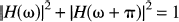
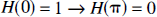
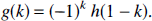
Where H(ω) is the FT of h( ). The filter g( ) is the modulated version of h( ) and is given by:

g (k) = (- 1)^{k} h (1 - k) .

(6)

The algorithm starts by passing the data through both filters h( ) and g( ) and then decimates their output by half (i.e., one every two output points is discarded). The high-pass-filtered and decimated data are the wavelets coefficients d₁(k) for the finest resolution. The low-pass-filtered and decimated data are the coefficients of the scaling function c₁ (k). By re-applying h( ) and g( ) to the residuals c₁(k), one obtains the wavelet and scaling coefficients for the coarser resolution, and so on.

The inverse transform may be obtained simply by reversing the previous sequence, and by use of synthesis filters , which are the reflection of h( ) and g( ). The DWT is shown in Fig. 2.

FIG. 2.

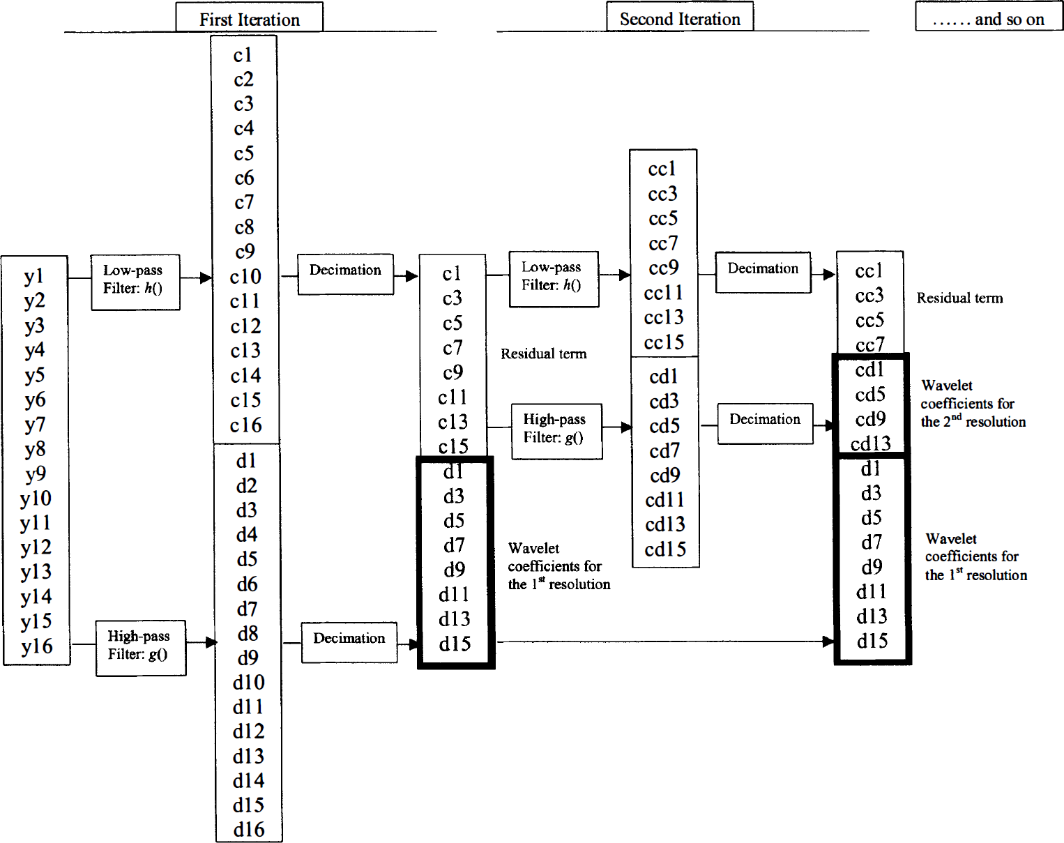
A general scheme of the dyadic wavelet transform. The original data (vector [y]) is filtered with the high-pass filter g() and then decimated to produce the wavelet coefficients for the first resolution (vector [d]). The residual coefficients, e.g., the coefficients of the scaling function for the first resolution (vector [c]), are obtained by convolution with the low-pass filter h( ) and subsequent decimation. The iteration of the filtering and decimation steps on the residual terms [c] produces the wavelet coefficients and the scaling coefficients for the second resolution level (respectively, vectors [cd] and [cc]). One can then iterate the filtering and decimation steps on the residual terms until the wavelet decomposition at the desired resolution level is obtained.

The DWT in two dimensions (2D-DWT) may be computed by applying the one-dimensional decomposition algorithm successively along the rows and columns of the image (Mallat, 1989). Therefore, the first iteration of the 2D-DWT algorithm generates four quadrants. The lower right quadrant (D) contains the so-called diagonal wavelet coefficients, and is obtained by use of the high-pass filter g( ) along rows and columns. The lower-left quadrant (V) contains the vertical coefficients generated by application of h( ) along the rows and g( ) along the columns. The horizontal coefficients, obtained by filtering the columns with h( ) and the rows with g( ), are stored in the upper-right quadrant (H). The upper-left quadrant (R) contains the residual coefficients of the scaling function, that is the coefficients obtained by applying h( ) to both rows and columns. The wavelet expansion for the coarser resolution is obtained by reapplying the above filtering steps to this quadrant. The first step of this recursive decomposition is shown in Fig. 3.

FIG. 3.

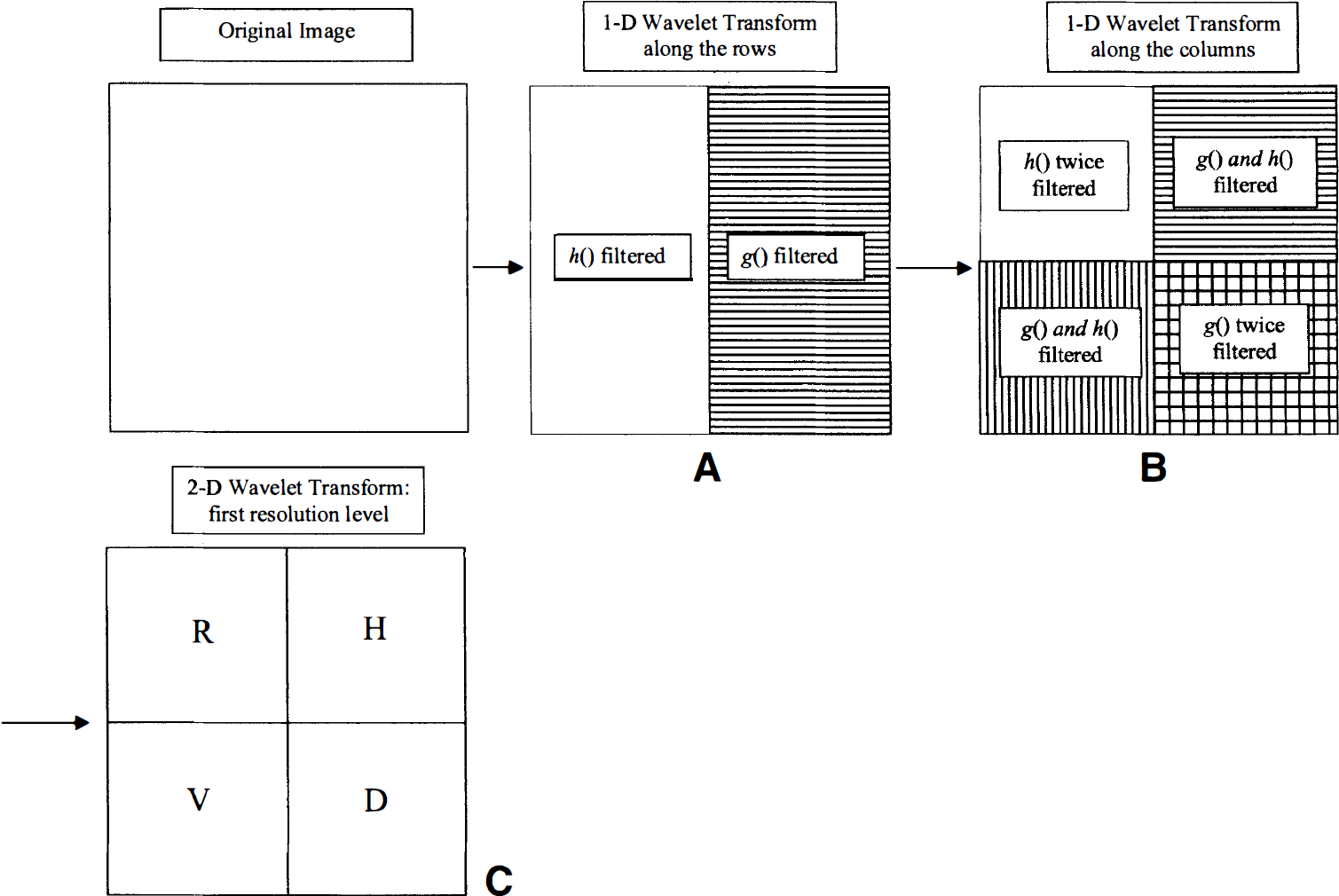
One iteration of the dyadic wavelet transform in Fig. 2D. (1) The one-dimensional transform is applied along the rows by application of the two filters g( ) and h( ) and subsequent decimation. This splits the columns in two halves (A). (2) The one-dimensional transform is applied to the columns splitting the rows into two halves (B). The final output is made of four quadrants labeled D (diagonal), H (horizontal). V (vertical), and R (residual) (C). The wavelet transform for the second resolution level is obtained by application of the above procedure to quadrant R.

The above framework can be easily extended to the N-dimensional case. The DWT in N dimensions (ND-DWT) may then be generated by sequential application of the DWT to each of the N axes. At each resolution this will generate 2^N quadrants. The transform of the coarser resolution can be obtained by reapplying the filters at the residual quadrant, as explained before.

For a detailed description of the theory and practical implementation of the DWT, the interested reader is referred to the original article of Mallat (1989). The material of Aldroubi (1996), Unser (1996) and Press et al. (1992) is also suggested for a general introduction to the subject.

CHOICE OF THE OPTIMAL WAVELET BASE

A wavelet base designed for application to ET images would ideally require the following properties. The base should be orthogonal to preserve the noise attributes of the spatial domain in the wavelet domain (see the section on Wavelets and Noise). Secondly, the wavelet function should be symmetric to avoid phase distortions and maintain more faithful signal localization in the wavelet domain (Ruttiman et al., 1998). The autocorrelation of the wavelet coefficients within each resolution level should die away rapidly; qualitatively this is a consequence of the ability of the wavelet base to represent the signal (see the section on Wavelet Basis Functions). Finally, to maximize the detection sensitivity, the WT should minimize the correlation between the wavelet coefficients at different resolutions (Ruttiman et al., 1996); this is achieved by minimizing the spectral overlap between the wavelet coefficients at different levels (Fig. 1).

Previous work on this subject (Unser et al., 1995; Ruttiman et al., 1996) has focused attention onto the polynomial spline (or Battle-Lemarie) wavelets (Mallat, 1989; Battle, 1987; Lemarie, 1988). These wavelets are orthogonal and symmetric and changing the polynomial degree of the spline n may modulate their time-frequency properties. In the limit n → ∞, the spline wavelets tend to be less localized in the time domain, as they get smoother, but their localization in the frequency domain increases as they approach the modulated sinc-wavelet, that is a perfect band-pass filter.

Therefore, the desirable properties of decorrelation between and within wavelet levels, described above, can be achieved for the Battle-Lemarie wavelets by a compromise on the selection of n. A small polynomial degree implies sharper wavelets that are better suited for the representation of local discontinuities of the signal (i.e., bumps); such a choice reduces the correlation between adjacent wavelet coefficients in the same level. Larger values for n reduce the overlap in the frequency domain between wavelet functions at different resolutions, and this translates into negligible correlation between levels.

Ruttiman et al. (1996) have shown that, for the application of PET images, an optimal balance between these two properties may be reached by use of orthogonal cubic-spline wavelets.

The compliance of a wavelet base to the above described optimality conditions may be translated to another property of interest both practical and theoretical: sparsity. To define this property, we may start by observing that the efficiency of a transform method in the solution of the estimation problem of Eq. [1] is directly proportional to the parsimony of the representation produced (Donoho, 1993). In other words, an optimal or near-optimal mathematical transform should be able to condense the information of the original signal or image into few large coefficients of its functional base. Ideally, the number of non-null coefficients should be the minimum if the functional space of the transform is an unconditional base for the signal of interest (Donoho, 1993). This is the sparsity property of unconditional bases. In the case of ET images, the optimality or near-optimality properties of orthogonal cubic-spline wavelets to represent a ET image should be mirrored by the degree of compression of images in the wavelet space. These properties are shown by the example of Fig. 4. A synthetic image of a Shepp-Logan phantom, without noise, was smoothed with a Gaussian filter with full width at half maximum (FWHM) = 8mm to simulate a perfect PET image. The 2D-DWT was applied to the image using a Battle-Lemarie wavelet base. The resulting wavelet transform contained a small number of big coefficients plus a large number of negligible ones. Their suppression brought no apparent loss of information as it is shown by the comparison of the original image with the one reconstructed from this reduced set of coefficients (Fig. 4). The ratio between the number of non-null wavelet coefficients and the number of non-null pixels in the original image was 0.05. This corresponds to a 95% compression rate that is a usual result for wavelets when used as a tool for image compression (Polchlopek and Noonan, 1997). Figure 5 shows a numerical evaluation of compression rate in the wavelet domain toward the correspondent error for the same image; the loss of information is computed as the sum of the squared differences between the original and the reconstructed image.

FIG. 4.

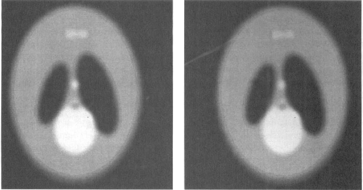
Illustration of the parsimony of the representation of a PET image in the wavelet domain. The left panel show a (256 × 256) synthetic image of a Shepp-Logan phantom that was smoothed with a Gaussian filter (full width at half maximum 8 mm) to represent a “perfect” PET image. The panel on the right shows the same image reconstructed from a set of wavelet coefficients that were 5% of the non-null pixels in the original image.

FIG. 5.

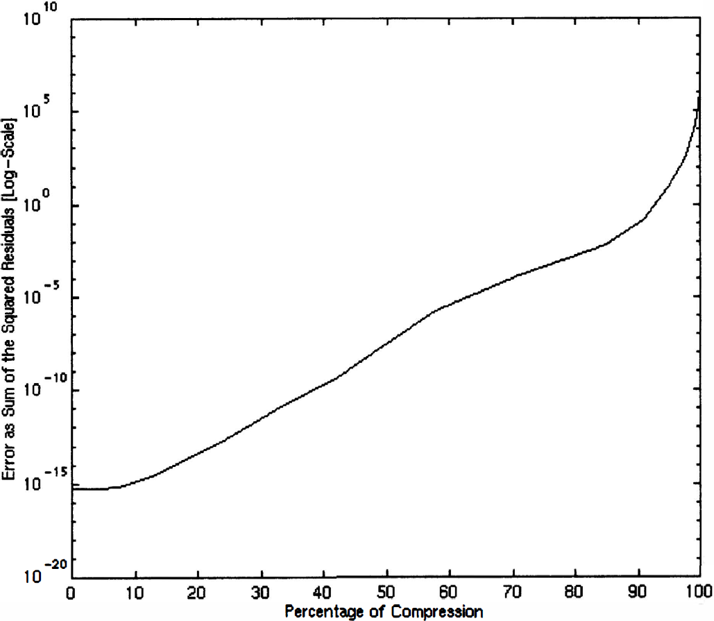
The plot of the ratio of compression (x-axis) toward the error for the example of the Shepp-Logan phantom. The error is expressed as the logarithm of the sum of the squared differences between the original image and the ones reconstructed by increasingly smaller (higher compression) sets of wavelet coefficients. The loss of information is negligible for compression rates until 95%. This indicates that a small number of wavelet coefficients are sufficient to model the signal in the simulated PET image.

WAVELETS AND NOISE

The orthogonality of the DWT has a fundamental statistical consequence: it transforms white noise into white noise (Donoho and Johnstone, 1994). Let d_j(k) be the wavelet coefficients for the signal F(t) (Eq. [4]). If we define w_j(k) as the coefficients of the wavelet transform of the noisy data Y(t) of [1], then we can write:

w_{j} (k) = d_{j} (k) + z_{j} (k)

(7)

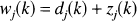
where Z_j(k) is a noise sequence ∼ N(0,σ²). That is, DWT maps the noise process e(k) of the original data (Eq. [1]) into the noise process z_j(k) on the wavelet coefficients that is normally distributed and has the same variance (only the wavelet coefficients d_j(k) and not c_j(k) are of interest for the statistical analysis).

The data compression remarks in the section on Choice of the Optimal Wavelet Base have emphasized that most of the coefficients in a noiseless wavelet transform are effectively zero. One can then re-formulate the problem of recovering F(t) as one of recovering those few wavelet coefficients of F(t) that are significantly non-zero, against a Gaussian white noise background (Donoho and Johnstone, 1994). Therefore, a suitable heuristic would be to find an estimate of the noise level, and then threshold the wavelet coefficients by use of appropriate rules and threshold values (Donoho and Johnstone, 1994). Such an approach is detailed in the following subsections.

Estimation of the noise variance

When the noise variance σ² is not known a priori, an estimate of it can be obtained directly from the wavelet coefficients. At fine resolution levels only a few wavelet coefficients are representative of the signal and is then possible to use a robust estimator for the standard deviation (SD) such as:

\hat{σ} = MAD {w_{j} (k), k = 1, \dots, 2^{j}} / 0.6745

(8)

where MAD denotes median absolute deviation from 0, w_j(k) are the wavelet coefficients of resolution level j and the factor 0.6745 is chosen for calibration with the normal distribution (Donoho et al., 1995).

Thesholding policies

The first step of a thresholding policy is the choice of the threshold function. Two standard choices are hard and soft thresholding (Donoho, 1995a; Donoho et al., 1995): given a wavelet coefficient w and a threshold t, the corresponding transformations are:

T^{hard} (w, t) = w I (| w | > t),

(9a)

T^{soft} (w, t) = sgn (w) (| w | - t) I (| w | > t),

(9b)

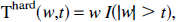
where I( ) is the indicator function. Hard-thresholding is a “keep-or-kill” strategy whereas soft-thresholding is a “shrink-or-kill”. Hard thresholding preserves the amplitude of the wavelet coefficients (i.e., is unbiased) at the cost of noisy artifacts that are due to the brisk separation between noise and signal. Soft thresholding reduces the variance due to such artifacts at the cost of an increase in bias as the coefficients are all reduced by an amount equal to t.

Once the type of thresholding has been selected, the next step consists of the choice of the threshold. The statistical literature on this subject is extensive and only some standard methods are here reviewed.

Universal threshold

Donoho and Johnstone (1994) proposed the threshold labeled universal that, for a set of M wavelet coefficients, is defined as:

t^{U} = \hat{σ} sqrt (2 \log M) .

(10)

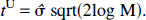
The rationale is to remove all wavelet coefficients that are smaller than the expected maximum of an assumed normal noise sequence of a given size M. The use of t^U ensures a noise-free reconstruction and it is easy to compute, but it tends to underfit the data (Nason, 1996).

This feature may be expected because t^U produces the best estimate in the minimax sense (Donoho and Johnstone, 1994). In other words, the rejection of all the wavelet coefficients that are less than t^U leads to the estimation of a function that is the solution of the problem defined in Eq. [1] when it is desired to minimize the maximum risk .

Bonferroni and Bonferroni-like corrections

From the statistical viewpoint, thresholding is equivalent to testing the hypothesis that each coefficient w is generated by a null normal distribution (Abramovich and Benjamini, 1996), that is w ∼ N(0,σ²).

This framework is often designated as “the multiple comparison problem” (Hochberg and Tamhane, 1987). The choice of threshold depends on the number of false-positive results that may be generated by the whole set of tests. The larger the number of tests, the higher is the expected number of false-positive results, so the threshold must be raised accordingly. The probability of a false-positive result is usually designated as Type I error. To control the multiplicity effect when considering a family of comparisons simultaneously, classical multiple comparison procedures seek to control the probability of committing any Type I error. The control of this family-wise error (FWE) implies that the probability of false rejection of at least one null hypothesis should be less than the error level a (Hochberg and Tamhane, 1987, p.7).

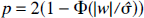
A simple procedure that controls the FWE at level a is the Bonferroni procedure that allows the rejection of one null hypothesis in a set of M tests if:

p < α / M

where:

p = 2 (1 - Φ (| w | / \hat{σ}))

and φ( )) is the standard cumulative normal distribution. Other Bonferroni-type procedures are available. For a review of these methods see Westfall and Young (1993). According to this framework, one can select a value for the FWE (e.g., α = 0.05) and then compute the threshold:

t^{Bonf} = \hat{σ} Φ^{- 1} (1 - α / 2 M) .

(11)

This approach and the universal approach described in the previous section are similar as they both aim at some control of the Type I error. Also similar are their thresholds: e.g., for values of M between 100 and 1000 the value of t^U corresponds to an overall probability of false-positive results α∼0.1.

Level-wise testing

Ruttiman et al. (1996) have suggested the practice of testing globally each resolution level by use of a chi-square test. If a wavelet level contains M coefficients w ∼ N(0, 1), then their sum of squares will be chi-square distributed with M degrees of freedom.

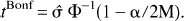
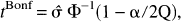
If the null hypothesis of any signal in that wavelet level is not rejected, than all the coefficients at that level are zeroed. Otherwise, one can test each coefficient independently as explained in the section on Bonferroni and Bonferroni-like Corrections. This procedure is designed to avoid unnecessary testing and thus reduce the Bonferroni threshold to:

t^{Bonf} = \hat{σ} Φ^{- 1} (1 - α / 2 Q),

where Q < M is the number of coefficients in all those levels where the chi-square test rejected the null hypothesis. Experimental evidence (Lau and Weng, 1995) suggests that stationary significance tests, such as the chi-square, are not sensitive enough to detect signal when it is represented by a few coefficients in large noise sequences. Thus, in the wavelet domain, their use may cause an overall loss of power.

Stein's risk estimator

The universal and Bonferroni-like thresholds are designed to minimize the probability of including noise in the reconstruction. These approaches minimize the variance of the solution at the cost of bias because part of the signal will be wiped out.

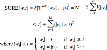
An unbiased approach to the minimization of risk considers the problem in the more general context of multivariate normal decision theory. The set of wavelet coefficients w = (w_i, …, w_M), previously normalized by division for , is considered a sample of a multivariate variable distributed ∼ N(μ_i, 1). The aim of the thresholding procedure is the estimation the vector μ = (μ₁,…, μ_M). Stein (1981) showed that any estimator of μ, either linear or non linear, biased or unbiased, has a correspondent risk that can be computed. Donoho and Johnstone (1995) derived a formula for the risk of the soft threshold T^soft(w,t):

\begin{aligned} SURE (w, t) & = E | T^{soft} (w, t), - μ |^{2} = M - 2 \sum_{i = 1}^{M} I (| w_{i} | \\ < t) + \sum_{i = 1}^{M} (| w_{i} | \land t)^{2} \\ where | w_{i} | \land t & = {\begin{cases} | w_{i} | = t & if | w_{i} | \leq t \\ | w_{i} | = | w_{i} | & if | w_{i} | > t \end{cases} \end{aligned}

The threshold can then be defined as the one value that minimizes the risk:

t^{SURE} = min (SURE (w, t)) 0 \leq t \leq t^{U}

(12)

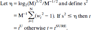
The use of t^SURE is generally very efficient but not very robust in cases where the signal is very sparse (Donoho and Johnstone, 1995). To overcome this limitation, it is suggested to test the set of coefficients before the computation of the threshold. If the test suggests extreme sparsity, then the universal threshold t^U must be preferred over t^SURE (Donoho and Johnstone, 1995). In detail, the test runs as follows.

\begin{aligned} Let η = & \log_{2} (M)^{3 / 2} / M^{- 1 / 2} and define s^{2} \\ = & M^{- 1} \sum_{i = 1}^{N} ({w_{i}}^{2} - 1) . If s^{2} \leq η then t \\ = & t^{U} otherwise t = t^{SURE} . \end{aligned}

The use of t^SURE allows the estimation of J in the least squares sense; in practice, this means that an estimate of the signal is produced that is less smooth than the one produced by t^U, at the expense of including some noise in the reconstruction (Donoho and Johnstone, 1995).

Other approaches to the treatment of noise in the wavelets domain may also be of interest. Nason (1996) applies the framework of cross-validation that has interesting properties in the non-normal case. The Bayesian point of view is outlined in Abramovich et al. (1998). Polchlopek and Noonan (1997) consider the problem in the context of signal-processing theory.

THEORETICAL AND NUMERICAL DEVELOPMENTS FOR EMISSION TOMOGRAPHY

The results of the previous sections have shown that WT techniques allow the estimation of a nonstationary signal in N-dimensions in a rigorous statistical framework. Their properties can then be proposed for the analysis of images of ET. In this particular context, no proper estimation approach exists and analysis is usually undertaken by monoresolution approaches: i.e., images are filtered before or after reconstruction by use of a filter of fixed resolution.

Two main difficulties hamper the use of WT in this field. The first one is due to the assumption of “white noise” in WT methodology that emphasized all the developments noted within the first part of this article. This assumption is not tenable given the correlation among pixels introduced by the image reconstruction process of the ET camera. The section on Theoretical and Numerical Developments for ET develops a colored noise model and suggests computing schemes that adapt to the amount of available information on the noise covariance function.

The second problem that one may encounter in the use of WT with ET is that usually, in these images, the signal is sparse and noise levels are high. Such signals are known to be unsuitable for WT as a number of artifacts are generated on reconstruction. Recent literature (Coifman and Donoho, 1995) has pointed out that these problems are due to the fact that the usual estimation process of the DWT is not translation invariant. There is arbitrariness in the way the decimation process is performed. In the algorithm of DWT of Fig. 2, the decimation step discards every even member of each vector sequence; this is not equivalent to a DWT where every odd member is discarded. It can be shown that the odd-decimation DWT is equal to the even-decimation DWT when a circular shift is previously applied to the data (Coifman and Donoho, 1995). This limitation of traditional DWT methods is particularly evident in cases with sporadic discontinuities and low signal-to-noise ratios where the algorithm may completely miss the signal (Johnstone and Silverman, 1997). Coifman and Donoho (1995) have developed a second-generation DWT for one-dimensional signals that enjoys the translation invariant property. This approach in 2 and N dimensions is developed in Translation-Invariant Wavelet Transform (see below).

Colored noise model

The properties of WT have interesting consequences when the transform is applied to a correlated noise process. We have shown previously (see the Choice of Optimal Wavelet Base) that the choice of a proper wavelet base allows a complete decorrelation between and within resolution levels. This means that if the noise process on the data is normally distributed but correlated, the resulting noise process in the wavelet space will be normally distributed and uncorrelated.

Unfortunately, the noise variance of the wavelets coefficients will not be the same as that of the data. Instead it will depend on the quadrants of the transform but will be constant within each quadrant (Johnstone and Silverman, 1997).

This can be understood by looking at DWT as a filtering process in the frequency space. At each step of the transform, the wavelet coefficients d(k) and the residuals c(k) are produced by the filters g( ) and h( ). It was observed before that their FT partition the power spectrum of the data in two almost not overlapping portions (Fig. 1). In the case of white noise, the noise spectrum is constant on all frequencies and the two portions filtered by g( ) and h( ) will then contain the same noise power. Therefore, the variance of the noise for d(k) and c(k) will be the same as that of the original data.

Instead, the spectrum of colored noise is not constant but varies according to the FT of its covariance function. Each filtering step will then select different portions of the noise spectrum and the noise variance of the coefficients will differ depending on the filters used (Johnstone and Silverman, 1997).

Therefore all the noise treatments discussed in the section on Wavelets and Noise can be applied to the DWT of a correlated noise process but the variance of the wavelet coefficients must be computed independently on each quadrant (Johnstone and Silverman, 1997).

The remaining issue is how to estimate the variance on each level. Three different cases are envisaged and will be described in the following sections. The sections on ET Images: Covariance Function Unknown and ET Images: Gaussian Correlation Function deal with the case of standard ET images and distinguish the case when a model for the point-spread function of the ET camera is available from the case when it is not. The section on Statistical Maps: Correlation Function Known deals with the special case of statistical maps that are derived from PET images.

All theoretical developments rely on the following assumptions. (1) Data are normally distributed. (2) The noise correlation structure is stationary; this implies that the point spread function of the scanner is equal in all the pixels. (3) The variance is constant across the image. Worsley et al. (1996) discuss these assumptions in the context of PET images.

Emission tomography images: covariance function unknown

It is supposed that a ET image is given and no estimate is available of the noise covariance function. This estimate cannot be computed directly from the image, as it would be biased by the presence of signal.

In this case, the only option is to use the robust estimator of Eq. [8] on the quadrants of each resolution level. We can rewrite [8] as:

{(\hat{σ})_{J}}^{Q u a d} = MAD (w_{J} (k), k \in Q u a d} / 0.6745,

(13)

Quad labels one of the quadrants at resolution J.

This estimate has a limitation; it is usually unbiased in the first resolution levels as the wavelet coefficients are mainly due to noise. At coarser resolution levels, the coefficients become fewer and an increasing proportion are due to the signal; this may lead to an overestimation of the SD of the noise. For ET images with pixel size of ∼ 2 mm, experience suggests that such an estimate may be valid only for the first two fine resolution levels.

Emission tomography images: Gaussian correlation function

This section considers the case when there is a model for the point spread function of the scanner. For example, a common approximation is the adoption of a Gaussian correlation function with a certain FWHM (Worsley et al., 1996). If there is a model for the correlation function, then an alternative procedure can be derived for computing the variance of each wavelet quadrant .

Let Corr(x) be the correlation function of the image that is supposed known. Let x be a N-dimensional vector. The covariance function Cov(x) is by definition:

C o v (x) = σ^{2} C o r r (x) .

(14a)

By definition also

C o r r (0) = 1 and C o v (0) = σ^{2} .

(14b)

This is true also in any quadrant at any resolution J, that is:

{C o v_{J}}^{Q u a d} (x) = σ^{2} {C o r r_{J}}^{Q u a d} (x) .

(15a)

{(σ^{2})_{J}}^{q u a d} = {C o v_{J}}^{Q u a d} (0) = σ^{2} {C o r r_{J}}^{Q u a d} (0)

(15b)

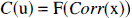
We also introduce the FT of correlation functions, that is:

C (u) = F (C o r r) (x))

and

{C_{J}}^{Q u a d} (u) = F ({C o r r_{J}}^{Q u a d} (x)) .

Let us now consider the ND-DWT. The wavelet coefficients of a certain quadrant at a resolution J, are obtained by applying h( ) and g( ) in a certain sequence and subsequent decimation. The decimation step allows the iterative use of h( ) and g( ) for all resolution without the need for their dilation (Mallat, 1989).

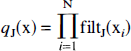
Instead, for our purposes, we will define the filters h_J ( ) and g_J( ) that are the dilated versions of h( ) and g( ) at each resolution J. They can be obtained by linear interpolation of the original filters h( ) and g( ). Hence, apart from the decimation step, each quadrant of the ND-DWT can be seen as derived by consecutive convolutions of the original image with N-dimensional filters:

Q_{J} (x) = \prod_{i = 1}^{N} {filt}_{J} (x_{i})

(40)

where filt_J(x_i) represents the filter used for dimension i at resolution j.

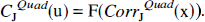
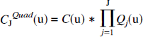
Let Q_J(u) = F(q_J(x)) and observe that convolution between two vectors is equivalent to the product of their FT. It can be shown that the correlation function of a filtered ET image is given by the product of the FT of the point-spread function of the scanner with the FT of the filters used (Worsley et al., 1996). It follows that the FT of the correlation function of a quadrant, at a resolution J, is given by the product of the FT of the point-spread function of the scanner with the FT of the filters used to obtain that particular quadrant, that is:

{C_{J}}^{Q u a d} (u) = C (u) * \prod_{J = 1}^{J} Q_{J} (u)

(17)

By application of Eq. 17, and subsequent inversion of the FT, one can obtain the correlation functions Corr_J^Quad (x) for all the quadrants; hence, the coefficients Corr_J^Quad(0) are known. To compute the variance of the quadrants from Eq. 15b, the remaining step is compute the variance of the image σ².

We suggest the following. First, obtain estimates of (σ²)_J^Quad for the quadrants of the finest resolution levels by application of the robust operator of Eq. 13, as detailed in the section on ET Images: Covariance Function Unknown. Secondly, suppose that P of these estimates are available. Insert them in Eq. 15b and produce a set of P equations with the noise variance σ² as unknown variable. Once σ² has been computed, re-apply Eq. 15b to the remaining quadrants at coarser resolutions and obtain the remaining estimates for ((σ²)_J^Quad.

The validity of this approach depends on how reliable the estimate is for the point-spread function of the scanner. Gaussian models are usually good first approximations and serve the purpose efficiently. In practice, in analogy with other applications (Donoho et al., 1995), we determined that on a PET image with pixel size ∼ 2 mm acquired with a modern PET scanner with resolution < 8 mm, one may estimate σ² by use of Eq. 15b at the first and second resolution levels, as most of the coefficients of these resolutions are due to noise. The estimate obtained can then be re-used efficiently to compute the variance of the remaining quadrants, as explained.

Only the first three to four resolution levels are of interest for the thresholding procedures. At higher resolutions, each non-null wavelet coefficient represents an object in the image of size greater than 2 mm × 2⁴ = 32 mm; such an object can be safely assumed to be due to signal.

Statistical maps: correlation function known

This section considers WT in the context of the analysis of statistical parametric maps (SPM). These maps are usually produced by collecting results of univariate tests (Student t-tests or their equivalent) computed on each site of the images (pixel), images that are acquired under different experimental conditions in different subjects. For the pixel to represent the same anatomical location for all subjects under every condition, images usually undergo a number of manipulations and are mapped into a standardized coordinate space that accounts for differences in brain size and orientation (Friston et al., 1991, 1995; Worsley et al., 1992). Finally, the locations of the images affected by the experimental condition are searched for by thresholding the maps. Values for the threshold are usually computed following criteria derived from the theory of Gaussian random fields (Friston et al., 1991; Worsley et al., 1992). These approaches usually search for the signal in a monoresolution fashion by smoothing the data with a Gaussian filter of fixed FWHM; Worsley et al. (1996) recently introduced a multiresolution approach that uses a number of different smoothings and sets the threshold accordingly.

WT methods approach the problem of the analysis of SPM differently. While the above techniques are intended to detect locations of the image that are significantly affected by the experiment, WT reconstructions show the significant profiles of activity caused by the experimental condition. In other words, WT approaches the problem from an estimation point of view, while random fields theory considers the problem in the context of hypothesis testing.

The application of WT to an SPM is no different from the application of WT to images. Statistical maps are transformed, the resulting wavelets are thresholded and then de-noised statistical maps are reconstructed (Unser et al., 1995; Ruttiman et al., 1996, 1998). Because the control of false-positive results is stringent in this application, the Bonferroni approach is suggested (see the section on Bonferroni and Bonferroni-1ike Corrections).

The computation of the variance for each quadrant of the WT is more straightforward for statistical maps than it is for images. First, the noise variance of the image σ² = 1, by definition of statistical map. Second, the correlation function can be easily computed because pure noise images are available. Pure noise images (or residual images) can be obtained by subtracting from the original scans the effects estimated through statistical analysis (Worsley et al., 1996). Once the residual images are obtained, Corr(x) can be computed through Fourier techniques. These techniques are detailed in Worsley et al. (1996) and will not be repeated here. Estimates of (σ²)_J^Quad for all resolution levels can then be directly obtained from Eq. 15b.

Translation-invariant wavelet transform

Coifmann and Donoho (1995) have described a wavelet de-noising procedure, termed cycle spinning, that enjoys the translation-invariant property.

The original tenet is to compute the DWT for all possible shifts of the data, de-noise each one of the computed DWT, invert them and average the results. At first sight, if the usual DWT is O(M), this procedure may seem O(M²) that is computationally unfeasible. Instead, it can be shown that at each resolution j, with j = 1, …, J, only 2^j circular shifts are needed (Coifmann and Donoho, 1995). This reduces the computational complexity to an acceptable O(M log(M)).

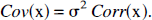
In the N dimensional case, the added dimensions implies that at each resolution level 2^{j + N} circular shifts are needed (Coifmann and Donoho, 1995). This section develops the cycle spinning algorithm in two dimensions. Extension to the N dimension is straightforward. The procedure works as follows (Fig. 6).

FIG. 6.

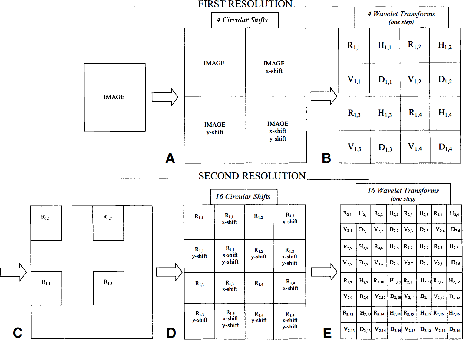
Illustration of the first two resolutions of the translation invariant 2D-DWT. At the first resolution level, four images are considered: the original image plus its three right shifts in the x-direction, in the y-direction and in both directions (A). Then, the first step of the 2D-DWT is applied to the four images producing four matrices, each divided in the usual four quadrants R, H, V, D (B). The wavelet coefficients of quadrants H, V, and D are stored. The remaining residual quadrants R are passed to the second resolution step (C). At the second resolution level, 16 images are considered, representing the four translations of the four residual matrices (D). One step of the 2D-DWT is then applied to the 16 images that produces 16 matrices divided in 32 quadrants. (E) The ones containing the wavelet coefficients are stored (quadrants H,V, D), the ones containing the residuals (quadrants R) are moved to the next resolution step.

At the first resolution, one iteration of the 2D-DWT is computed for four images. The first one is simply the original image. The other three are the images produced by application of a right circular shift first to all the rows, then to all the columns, then altogether to all rows and columns of the original matrix. This step produces the first level of the translation invariant 2D-DWT that is then made of four matrices, each divided in the usual four quadrants D, H, V, R.

The second resolution level is obtained by applying the above steps to each of the four R quadrants of the first resolution level. That is, one iteration of the 2D-DWT is applied to the four quadrants R and to the quadrants obtained by their rotational shift. This produces 4*4 = 16 matrices.

The procedure then iterates for all other resolution levels. The inverse transform algorithm starts from the coarsest resolution level and proceeds backwards until the original image is reconstructed. At each level, the usual inverse 2D-DWT is applied to each of the 2^{j + 1} matrices of that resolution. The results are then back-shifted and averaged to produce 2^j matrices that form the R-quadrants of the 2^j 2D-DWT of the finer resolution level.

The denoising of this transform can be performed simply by thresholding each resolution level using either prescription in the sections on Wavelets and Noise and the Colored Noise Model.

METHODS

The theoretical framework of the section on Theoretical and Numerical Developments for ET was applied to a number of experiments with synthetic data, statistical maps, and clinical PET images with various resolutions and signal-to-noise ratios. For experiments on a wider range of signals, the interested reader is directed to references cited in the above sections, particularly Nason (1996), Coifman and Donoho (1995), and Donoho and Johnstone (1994, 1995).

The software used for the computation was written in MAT-LAB (The Mathworks Inc., MA, U.S.A)* and run on an Ultra-Sparc 1 (143 MHz CPU) Sun Workstation (SunSystems, Mountain View, CA, U.S.A.).

Subroutines for the generation of the Battle-Lemarie filters and the computation of the one-dimensional DWT were taken from the Wavelet Toolbox Uvi-Wave 3.0 (Sánchez SG, Prelcic NG, Galán SJ, Grupo de Teoría de la Señal, Universidad de Vigo, Spain). The cubic spline Battle-Lemarie filter was used in all studies. Corresponding filters were constructed according to the implementation of Mallat (1989).

The 2D-DWT was used for the analysis of all images and statistical maps. Unless otherwise specified, the cycle-spinning transform was used in all experiments. The following sections detail the setup for each experiment.

Synthetic image

A simulation study was devised to investigate the property of the denoising procedures and evaluate their results in the case of a known signal. Besides, it was of interest to compare WT methods with the multiscale approach of Worsley et al. (1996) for the analysis of statistical maps.

One synthetic image (128 × 128) was generated that contained four circles of radius 4, 8, 16, 24 pixels, respectively. Height of the signal was l. White noise was added (SD = 1) and the image was smoothed with a Gaussian filter of FWHM = 4 pixels.

Because the pure noise image was available, the correlation function of the wavelet coefficients was computed for each resolution level as described in the section on Statistical Maps.

The denoising of the transform was performed at each resolution by use of both the SURE approach (see Stein's Risk Estimator) and the Bonferroni approach (see Bonferroni and Bonferroni-like Corrections). The Bonferroni threshold was set to control the FWE on all the resolutions at a significance α = 0.05.

For comparison, the multiresolution approach of Worsley et al. (1996) was used, with the same FWE α = 0.05.

Statistical maps

The activation study was chosen because of its robust and predictable activation signal in motor and visual areas. Subjects were scanned in one of three conditions; two activation and one rest. In all conditions subjects looked at a computer monitor displaying a series of stimuli, consisting of abstract designs and video clips of four abstract hand gestures. In the two activation conditions subjects performed one of the four abstract hand gestures with their right hand; they performed the gestures every 12 seconds in response to the stimuli. In the rest condition they were told to observe the stimuli without moving, and to let their minds go blank. For each subject there were two rest scans and 10 activation scans. Previous analysis with standard SPM96 software (Functional Imaging Laboratory, London, U.K.) had shown significant differences between activation and rest, but trivial differences between the activation conditions (Brett et al., 1998). The two activation conditions have therefore been pooled in the following analysis.

Seven subjects were scanned with an ECAT 953B PET camera (CTI/Siemens, Knoxville, TN, U.S.A.). Approximately 9.2 mCi were of H₂O¹⁵ were injected by the bolus method for each scan. Data was acquired in 3D mode, using a standard acquisition and reconstruction protocol (Townsend et al., 1991). After reconstruction, scans for each subject were realigned to the first scan in the session for that subject using SPM96 software, and then coregistered to the MNI standard brain (Evans et al., 1993). For the coregistration, we used an updated version of SPM96, with routines implementing the Bayesian algorithms described in Ashburner et al. (1997). There was no smoothing applied the images before statistical analysis.

A statistical image was then generated according to the method of Worsley (1992). Scans were first adjusted for changes in global counts by dividing data for each pixel by the mean pixel count for that scan. For each subject, we generated an activation minus rest difference image by subtracting the mean of the rest scans from the mean of the activation scans. The mean of the resulting seven subtraction images was then divided by the pooled standard deviation for intracranial pixels to give a Z score image.

The variance of wavelets' resolution levels was computed by using the residual images as in the section on Statistal Maps. The denoising procedure adopted a Bonferroni threshold that controlled the Type I error at the level α = 0.05 for the whole volume of 24 slices.

Low-resolution SPECT study

This example applies wavelet filters to a low-resolution SPECT image. Given its intrinsic low resolution, we can expect the signal to be sparse; i.e., the image will contain only few smooth objects. Therefore, this is a good data set on which to compare the traditional 2D-DWT and the translation invariant approach. The SPECT images were acquired using a Hoffman brain phantom (Hoffman et al., 1990) and a state-of-the-art triple-headed gamma camera (PICKER 3000XP, Picker International Inc, Cleveland, OH, U.S.A.) equipped with fanbeam collimators. The phantom was filled with ^99mTc and images were acquired over 120° for each head to provide the necessary tomographic data for image reconstruction. Images were reconstructed using filtered back-projection with a ramp filter. A single slice was selected and used in the wavelet analysis.

For both methods, the variance of each quadrant was computed as described in the section on ET Images. A model of the point-spread function of the scanner was used that assumed a Gaussian shape with FWHM = 10 mm. Wavelet coefficients were hard-thresholded with the universal threshold.

High-resolution PET images

The aim of this example is twofold. (1) It is designed to show the ability of wavelet filters to adapt to increasing signal-to-noise ratios. (2) It allows the comparison of the universal (hard-thresholding) and SURE thresholds and of their estimation approaches, the minimax and least squares respectively.

Therefore, a dynamic [¹⁸F]fluorodeoxyglucose study of brain function measured with a ECAT 953B PET camera (CTI/Siemens) was considered. The wavelet transform was applied first to a slice of the last frame; then, to the same slice that was summed over the last eight frames to increase the signal-to-noise ratio. During this time interval (20 to 60 minutes after injection) most of the signal is due to the constant build-up of the tracer trapped in the tissue. The unbound portion of the tracer, at least the one in gray matter, is equilibrated with the tracer in the plasma and therefore is slowly decaying (Schmidt et al., 1996).

Following the previous characterization of the PET scanner (Spinks et al., 1992), the point spread function of the image (x-y plane) was assumed to be Gaussian shaped with FWHM = 6mm.

Very high-resolution PET images

Finally, we consider an application of the methodology to a high-resolution PET image with high signal-to-noise ratio from an EXACT 3D PET scanner (CTI/Siemens). The wavelet analysis was applied to a [¹¹C]PK11195 study of peripheral benzodiazepine receptors in the brain. The high signal-to-noise ratio was obtained by summing all the 18 frames of the dynamic acquisition. The point-spread function (x-y plane) was assumed to be Gaussian with FWHM = 4.5 mm following previous characterization of the scanner (Bailey et al., 1998). The SURE method for denoising was used.

RESULTS

Synthetic image

Figures 7, 8, and 9 show the raw data and the results of the experiment. It is of interest to observe the relationship between the image resulting from hypothesis testing (Fig. 7C) and the one obtained from reconstruction from a WT denoised with the Bonferroni approach (Figs. 7D and 9B).

FIG. 7.

Data and results of the synthetic image experiment. (A) The original image (128 × 128) consisted in four circles of radius, respectively, 4, 8, 16, and 24 pixels. The height of the signal was 1. (B) White noise was added (SD = 1) and the image was smoothed with a Gaussian filter of FWHM = 4 pixels. (C) The result of the multiscale hypothesis testing approach is a binary image. Pixels found significant at any smoothing are depicted in white. The statistical testing was performed in the spatial domain by use of corrections derived from random fields theory (overall Type I error level α = 0.05). (D) The result of wavelet filtering is the estimated map, i.e., the significant profiles of the image. The testing was performed in the wavelet domain by use of the classic Bonferroni method (overall Type I error level α = 0.05). Note that the image is denoised at the cost of the almost complete loss of the finest resolution signal.

FIG. 8.

The noisy image of Fig. 7 is here denoised using the SURE approach. The signal is mostly recovered at the cost of an increased noise level in the reconstructed image.

FIG. 9.

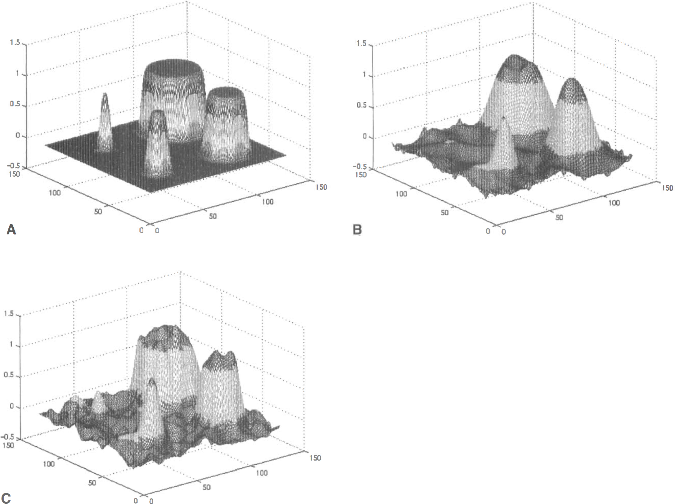
Mesh-plots of the original noise-free synthetic image (A), the image de noised by the Bonferroni approach (B) and the one denoised by the SURE approach (C). The Bonferroni approach produces a noise-free reconstruction. The cost paid is a nearly complete loss of the signal from the finest circle and an increased smoothness in the reconstruction. The SURE approach recovers most of the signal even at the finest resolution and produces a sharper reconstruction that is close to the original signal. The price paid is an increase in the noise level in the recovered image.

The results of the hypothesis testing approach are presented as a binary map where the significant pixels at any resolution are showed in white. The results of the wavelet approach, instead, are shown as estimated profiles of activity. This emphasizes the difference between a hypothesis testing approach and an estimation approach.

This relationship is mirrored in the results. Both approaches produce images that are noise free. The hypothesis testing approach detects the large signals although it overestimates their spatial size; this is due to over-smoothing by the largest filters. The WT approach, with the Bonferroni control of the error rate, estimates these signals but their reconstructions are slightly smoother than the original. The smallest circle reached borderline significance in the hypothesis testing approach and its signal was marginally recovered in the wavelet reconstruction.

The SURE approach, instead, departs from the control of the type-I error and aims to an optimal balance between variance (i.e., noise) and bias (i.e., signal recovery) in the reconstruction. Such an approach (Figs. 8 and 9C) preserves most of the sharpness and the height of the signal but the filtered image is noisier.

Statistical maps

The wavelet filtered statistic image is shown in Fig. 10. The filtered activation image is displayed in color overlaid on a gray scale magnetic resonance image of the MNI standard brain. The left side of the brain is to the left of the slices; slices are labeled with their distance in mm from the transverse plane containing the anterior and posterior commisures. The detected signal change was for the most part clearly defined and convincing. Complex hand gestures of the sort used in this study would be expected to activate the motor network, and this is well shown, with striking activation of the cerebellum (planes at −32 mm to −20 mm) and left motor cortex (36 to 48 mm). There was less striking but clear activation of the midbrain (−28 to −24), left ventral putamen / pallidum (−20, −16), left thalamus (−8, −4), motor cingulate (28–36) and bilateral somatosensory / parietal cortex (16 to 52). There is activation in primary and secondary visual cortex (−24 to −4), which may reflect increased attention to the visual stimuli during activation scans as compared to rest. There is also some apparent activation of low intensity in white matter at 4 mm which is presumably not physiologic. However, this may be detecting some of the complex signal change induced by prior processing, including image reconstruction, realignment, and coregistration.

FIG. 10.

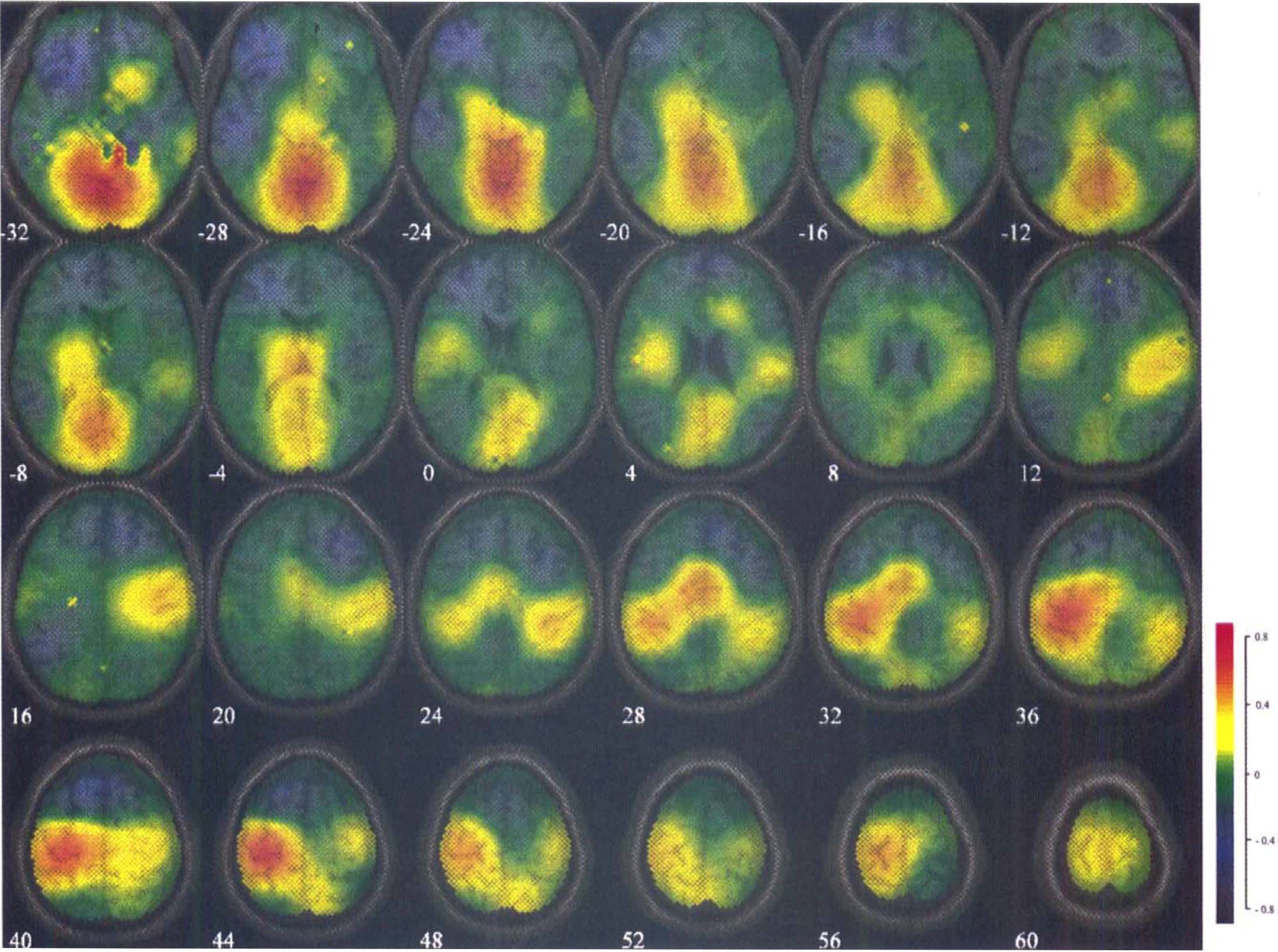
The figure shows the results of the wavelet procedure when applied to the analysis of a water activation study. The activation study was designed to activate the motor and visual areas. The filtered activation image is displayed in color overlaid on a gray scale magnetic resonance image of the MNI standard brain. Values represent the pattern of z-scores estimated with an error rate α = 0.05 over all 24 slices. The left side of the brain is displayed at the left of the slices. Slices are labeled with their distance in millimeters from the transverse plane containing the anterior and posterior commisures.

Figure 10 also shows an important advantage of the wavelet filtering approach over thresholding methods. This is the ability of the technique to show the definition of the signal change. For example, it appears from planes 40 mm and 44 mm that there is a sharp demarcation between motor cortex, which is activated, and the anterior premotor cortex, which is deactivated. The definition of this boundary probably reflects both the low variability of the position of the motor cortex from subject to subject, and the differences in activation between the motor and premotor cortex. In contrast, the posterior edge of the parietal cortex activation on the same planes is less distinct, which may be because there is greater variability of the boundaries of the parietal areas between subjects than there is for the motor cortex. This information is of course lost with images derived from thresholding methods.

Low-resolution SPECT study

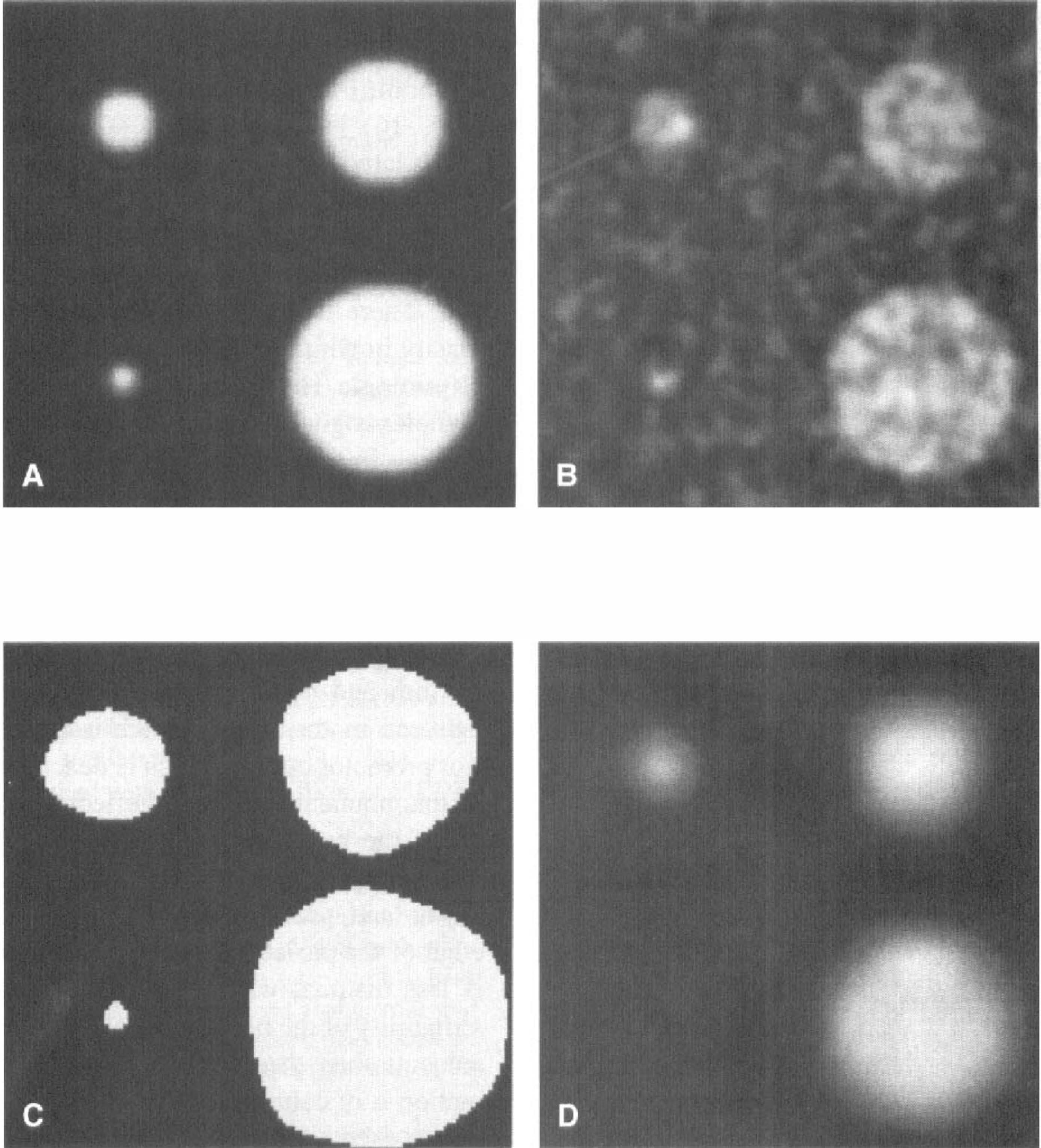
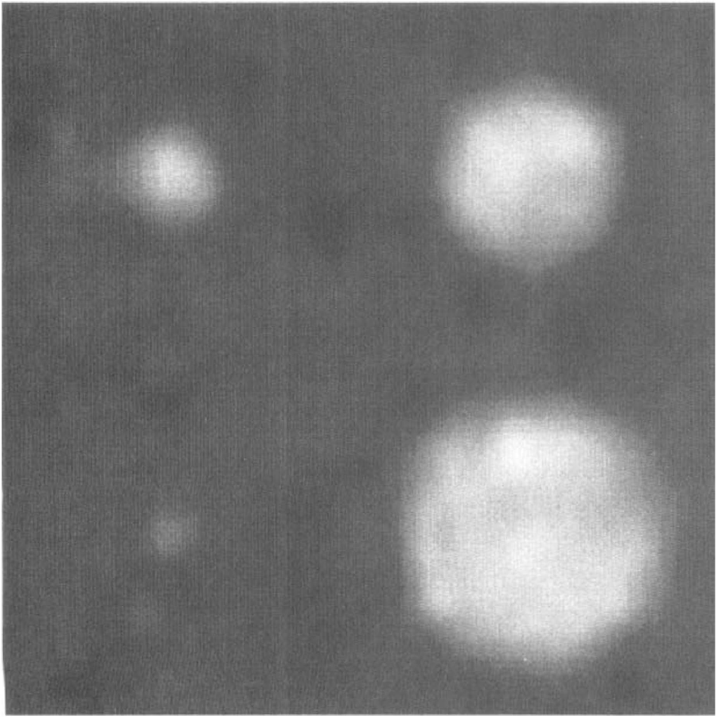
Figure 11 shows the data and results of the Hoffman-phantom experiment. Figure 11A shows the noisy image that was obtained by back-projection filtered with a ramp filter. This image was the input for the wavelet filters. Figure 11B shows the problems that one may encounter when the traditional 2D-DWT is used instead of the translation-invariant approach. The image not only contains artifacts but part of the signal is completely missing from the reconstruction. These effects are due to the decimation process in the algorithm that misses the signal, particularly when it is sparse. These results are similar to the ones obtained in one-dimensional problems (Coifman and Donoho, 1995).

Such artifacts disappear when the translation invariant algorithm is used (Fig. 11C).

FIG. 11.

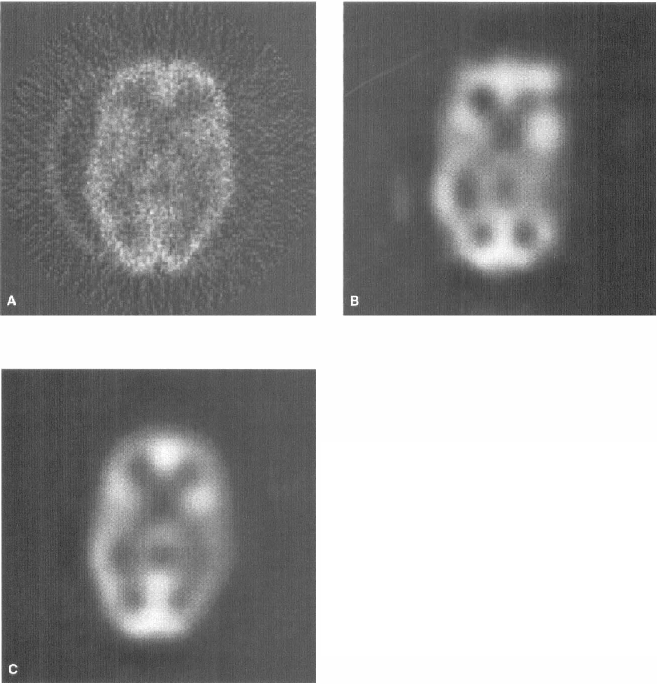
Data and results from the Hoffman-phantom experiment. The figure shows the original image (A), the reconstruction obtained with the traditional wavelet transform (B) and the one obtained with the translation invariant approach (C). The image (B) shows artifacts and part of the signal is missing. These errors are typical of the traditional wavelet transform when applied to sparse and noisy signal and justify the cycle-spinning approach developed in the text.

High-resolution PET images

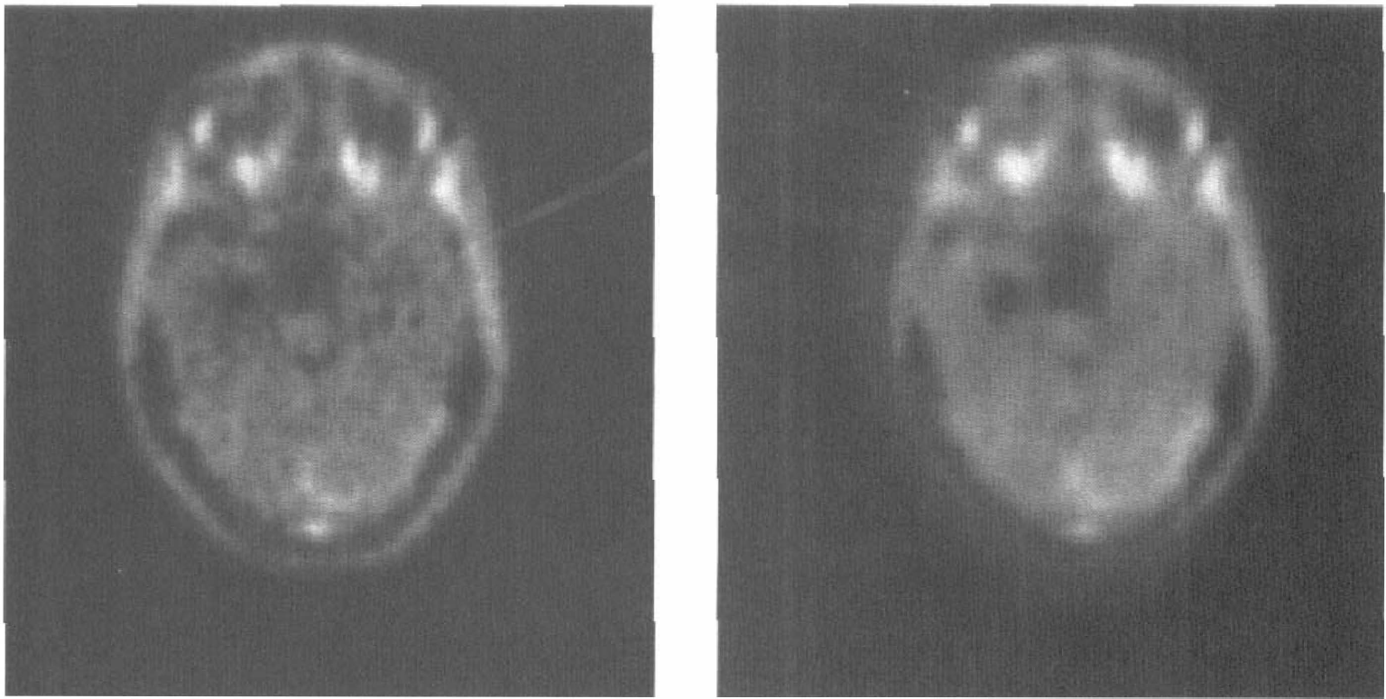
The results of the analysis of the [¹⁸F]fluorodeoxyglucose study are shown in Fig. 12. The filtering of the single frame (Fig. 12A), which has poor signal-to-noise ratio, resulted in high smoothing for both the universal filter (Fig. 12B), and the SURE filter (Fig. 12C). When the signal-to-noise ratio was increased by summing the last frames (Fig. 12D), both filters adapted to the increased signal levels. The universal filter (Fig. 12E) produced a sharper image while the SURE filter (Fig. 12F) detected details of the structures at the finest resolution. This example emphasizes the notion that, although the PET camera defines the lower bound of the resolution, the effective resolution is defined by the signal-to-noise ratio of the image

FIG. 12.

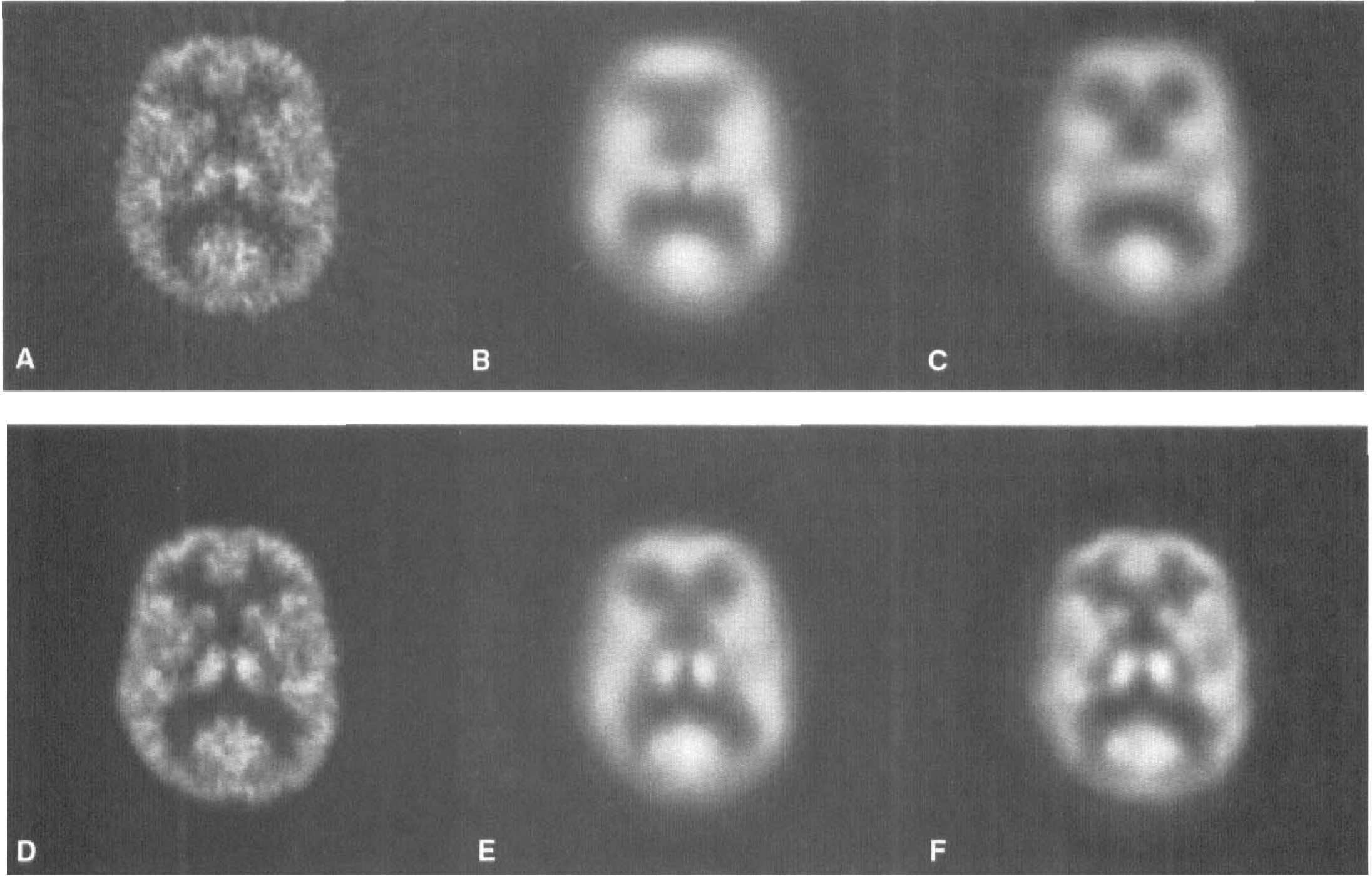
This example shows the ability of wavelet filters to adapt to increased information content in the image. (A) A slice of the last frame of a dynamic [¹⁸F]fluorodeoxyglucose study. (D) the same slice is summed over the last eight frames to increase the image signal-to-noise ratio. Both the universal filter (B,E) and the SURE filter (C,F) detect the increase of signal and produce a finer level of detail when noise level is lower

Very high-resolution PET images

Figure 13 shows the results of the application of the filters to the PK image. The original image (Fig. 13A) shows with interesting detail the distribution of the tracer. The least-square risk of the SURE filter (Fig. 13B) allows a consistent removal of the noise and the preservation of edges and details.

FIG. 13.

Wavelet analysis of a high-resolution image with high signal-to-noise ratio. (A) The frame was obtained by summing the 18 frames of a dynamic [¹¹C]PK11195 study. (B) The SURE filter is able to preserve edges and details and, at the same time, it removes a large proportion of the noise.

CONCLUSION

The current work aims to lay down a general framework for the analysis of ET images through wavelet-based methods. Three fundamental and equivalent aspects of data analysis were of interest: statistical estimation, optimal filtering, and data compression.

These are not usually addressed in ET data analysis. Current methods mainly rely on monoresolution approaches that smooth the image with filters of fixed FWHM (Unser et al., 1995). In the case of statistical maps, the features of interest of an image are searched by hypothesis testing approaches that do model the noise, but not the signal (Worsley, 1997).

Instead, proper wavelet bases allow the efficient modeling of the signal and the solution of the estimation problem in an unconditional-base setting (Donoho, 1993). This equally transposes into the ability of wavelet filters to automatically adapt, in a theoretically optimal manner, to the content of signal at different resolution levels. At the same time, the output of such filters corresponds to the optimal compression rate of the data.

The application of the wavelet transform to ET images translates the original problem of feature estimation in a random field into the classical problem of signal detection in white noise background. This rigorous statistical setting allows the solution of the estimation problem according to a variety of risk functions; their choice depends on the type of application.

Methods that strictly control the Type I error may be used in all those settings, like the analysis of statistical maps, where noise must be excluded from the reconstruction.

The SURE approach, instead, that has better mean square error properties, may be optimal for all those situations when absolute quantification of the image is paramount. Therefore, it is suggested that such filter may be of general use for clinical PET-SPECT images, particularly when the spatial pattern of distribution of the tracer is unknown.

The theoretical and numerical aspects that were developed here, addressed two technical difficulties typical of the application: (1) the presence of colored noise in ET images and (2) their low signal-to-noise ratio. The first problem was solved for a variety of cases depending on the knowledge available of the noise covariance function of the image. The second was approached by developing a translation-invariant procedure that eliminates the artifacts in the reconstruction that are typical of the traditional DWT.

The resulting framework may be considered of general use but of course, not definitive. The field of statistical methods for wavelets is in steady growth (Antoniadis and Oppenheim, 1995); newer and more powerful methods appear at a remarkable rate and they can be easily converted for this type of application.

We envisage that part of the future research should be directed at relaxing some of the assumptions about the noise structure of the image. Nonparametric approaches and models for local varying variance may be of interest in this context. Those applications where prior information on the spatial patterns of the signal is available may be also suitable for Bayesian approaches (Abramovich et al., 1998).

Finally, it is important to remark that the wavelet transform for ET images may have a number of optimality properties, but is not ideal. The ideal approach would be to apply wavelets not on images but directly on sinograms. Wavelet decomposition approaches to the inversion of the radon transform have been theoretically developed (Donoho, 1995b; Peyrin and Zaim, 1996) and applied to computerized tomography (Kolaczyk, 1996). Thus, an interesting effort would be to transfer the methods here developed for post-reconstruction filters directly into the image reconstruction process.

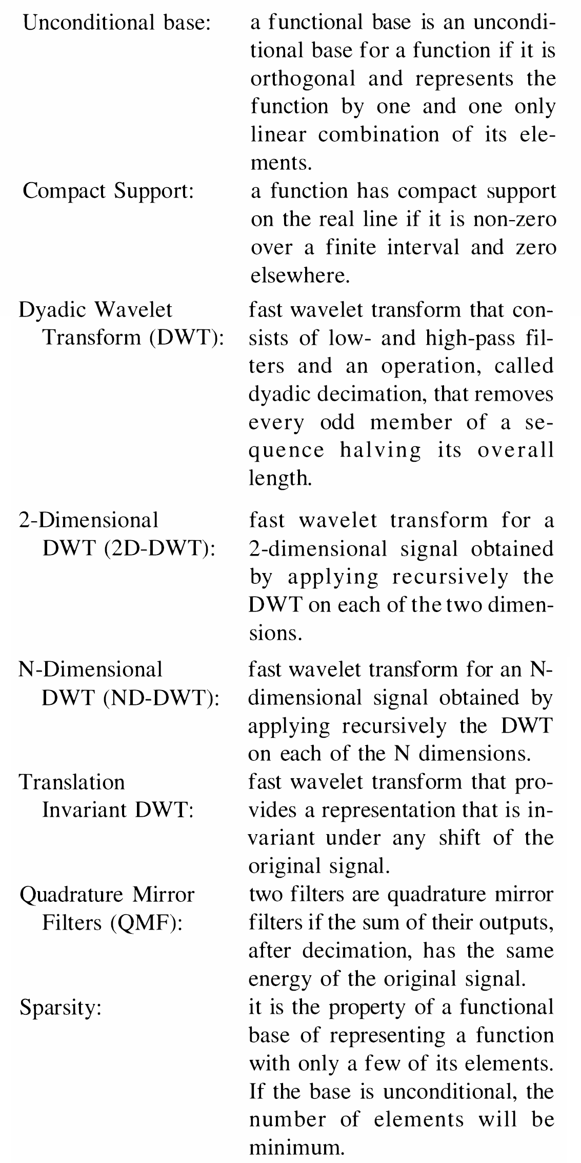
APPENDIX 1: TABLE OF DEFINITIONS OF TERMS SPECIFIC TO WAVELETS

Unconditional base:	a functional base is an unconditional base for a function if it is orthogonal and represents the function by one and one only linear combination of its elements.
Compact Support:	a function has compact support on the real line if it is non-zero over a finite interval and zero elsewhere.
Dyadic Wavelet Transform (DWT):	fast wavelet transform that consists of low- and high-pass filters and an operation, called dyadic decimation, that removes every odd member of a sequence halving its overall length.
2-Dimensional DWT (2D-DWT):	fast wavelet transform for a 2-dimensional signal obtained by applying recursively the DWT on each of the two dimensions.
N-Dimensional DWT (ND-DWT):	fast wavelet transform for an N-dimensional signal obtained by applying recursively the DWT on each of the N dimensions.
Translation Invariant DWT:	fast wavelet transform that provides a representation that is invariant under any shift of the original signal.
Quadrature Mirror Filters (QMF):	two filters are quadrature mirror filters if the sum of their outputs, after decimation, has the same energy of the original signal.
Sparsity:	it is the property of a functional base of representing a function with only a few of its elements. If the base is unconditional, the number of elements will be minimum.

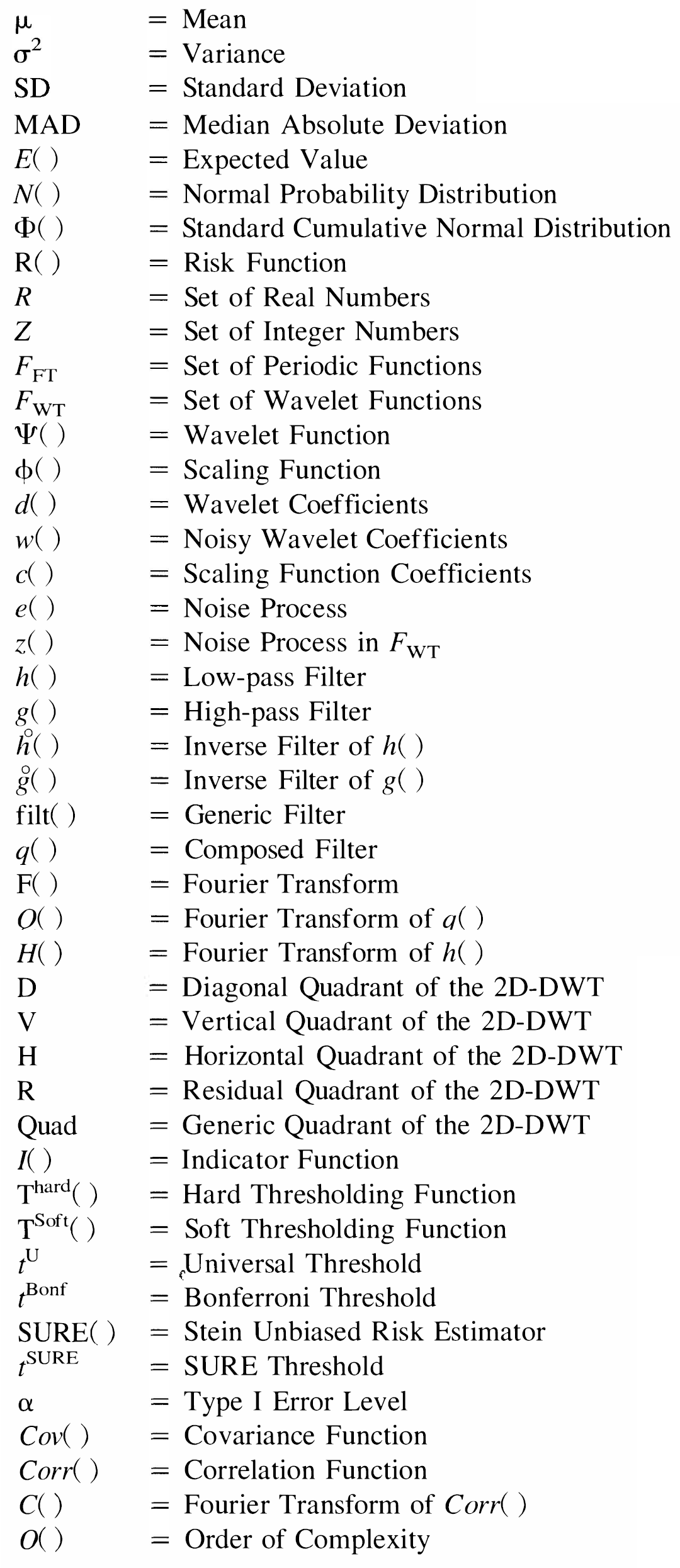
APPENDIX II: GLOSSARY OF SYMBOLS

μ	= Mean
σ²	= Variance
SD	= Standard Deviation
MAD	= Median Absolute Deviation
E( )	= Expected Value
N( )	= Normal Probability Distribution
φ( )	= Standard Cumulative Normal Distribution
R( )	= Risk Function
R	= Set of Real Numbers
Z	= Set of Integer Numbers
F _FT	= Set of Periodic Functions
F _WT	= Set of Wavelet Functions
Ψ( )	= Wavelet Function
φ( )	= Scaling Function
d( )	= Wavelet Coefficients
w( )	= Noisy Wavelet Coefficients
c( )	= Scaling Function Coefficients
e( )	= Noise Process
z( )	= Noise Process in F_WT
h( )	= Low-pass Filter
g( )	= High-pass Filter
	= Inverse Filter of h( )
	= Inverse Filter of g( )
filt( )	= Generic Filter
q( )	= Composed Filter
F( )	= Fourier Transform
Q( )	= Fourier Transform of q( )
H( )	= Fourier Transform of h( )
D	= Diagonal Quadrant of the 2D-DWT
V	= Vertical Quadrant of the 2D-DWT
H	= Horizontal Quadrant of the 2D-DWT
R	= Residual Quadrant of the 2D-DWT
Quad	= Generic Quadrant of the 2D-DWT
I( )	= Indicator Function
T^hard( )	= Hard Thresholding Function
T^Soft( )	= Soft Thresholding Function
t ^U	= Universal Threshold
_tBonf	= Bonferroni Threshold
SURE( )	= Stein Unbiased Risk Estimator
t ^SURE	= SURE Threshold
α	= Type I Error Level
Cav( )	= Covariance Function
Corr( )	= Correlation Function
C( )	= Fourier Transform of Corr( )
O( )	= Order of Complexity

Software available on request from the author.

Footnotes

Acknowledgments:

The authors thank Richard Banati for the provision of data, and Kris Thielemans and Suren Rajeswaran for fruitful discussion and helpful suggestions.

Abbreviations used:

References

Abramovich

Benjamini

(1996) Adaptive thresholding of wavelet coefficients. Computat Stat Data Anal 22:351–361

Abramovich

Sapatinas

Silverman

(1998) Wavelet thresholding via a Bayesian approach. J Roy Stat Soc B 85:115–129

Aldroubi

(1996) The wavelet transform: a surfing guide. In: Wavelets in medicine and biology. ( Aldroubi

Unser

, eds). Boca Raton. FL: CRC Press, pp 3–36

Antoniadis

Oppenheim

(1995) Wavelets and statistics. New York, NY: Springer-Verlag

Ashbumer

Neelin

Collins

Evans

Friston

(1997) Incorporating prior knowledge into image registration. Neuroimage 6:344–352

Bailey

Miller

Spinks

Bloomfield

Livieratos

Banati

Myers

Jones

(1998) Brain PET studies with a high sensitivity fully 3D tomograph. In, Quantification of brain function using PET. ( Herscovitch

Daube-Whiterspoon

Carson

, eds). San Diego, CA: Academic Press, pp 25–32

Battle

(1987) A block spin construction of ondelettes. Part I: Lemarie functions. Commun Math Phys 110:601–615

Bracewell

(1986) The Fourier Transform and Its Applications 2nd ed., New York: McGraw-Hill, pp 160–163

Brett

Stein

Brooks

(1998) The role of the premotor cortex in imitated and conditional praxis. Neuroimage 7:S978

10.

Coifman

Donoho

(1995) Translation-invariant denoising. Lect Notes Statist 103:125–150

11.

Daubechies

(1992) Ten Lectures On Wavelets. Philadelphia, PA: Society for Industrial and Applied Mathematics

12.

Donoho

(1993) Unconditional bases are optimal bases for data compression and for statistical estimation. Appl Comput Harmonic Anal 1:100–115

13.

Donoho

(1995a) De-noising by soft thresholding. IEEE Trans Inform Theory 41:613–627

14.

Donoho

(1995b) Nonlinear solution of linear inverse problems by wavelet-vaguelette decomposition. Appl Comput Harm Anal 2:101–126

15.

Donoho

(1996) Unconditional bases and bit-level compression. Appl Comput Harmonic Anal 3:388–392

16.

Donoho

Johnstone

(1992) Minimax estimation via wavelet shrinkage. Technical Report 402, Department of Statistics, Stanford University

17.

Donoho

Johnstone

(1994) Ideal spatial adaptation by wavelet shrinkage. Biometrika 81:425–455

18.

Donoho

Johnstone

(1995) Adapting to unknown smoothness via wavelet shrinkage. J Am Statist Ass 90:1200–1224

19.

Donoho

Johnstone

Kerkyacharian

Picard

(1995) Wavelet shrinkage: asymptopia? J Roy Stat Soc B 57:301–369

20.

Evans

Collins

(1993) A 305-member MRI-based stereotaxic atlas for CBF activation studies. J Nucl Med 34:70–71

21.

Friston

Frith

Liddle

Frackowiak

RSJ

(1991) Comparing functional (PET) images: the assessment of significant change. J Cereb Blood Flow Metab 10:458–466

22.

Fristan

Holmes

Worsley

Poline

Frith

Frackowiack

RSJ

(1995) Statistical parametric maps in functional imaging: a general linear approach. Hum Brain Mapping 2:189–210

23.

Hochberg

Tamhane

(1987) Multiple comparison procedures. New York, Wiley

24.

Hoffman

Cutler

Dygby

Mazziotta

(1990) 3-D phantom to simulate cerebral blood flow and metabolic images for PET. IEEE Trans Nucl Sc 37:616

25.

Johnstone

Silverman

(1997) Wavelet threshold estimators for data with correlated noise. J R Statist Soc B 59:319–351

26.

Kolaczyk

(1996) A wavelet shrinkage approach to tomographic image reconstruction. J Am Statist Assoc 91:1079–1090

27.

Lau

Weng

(1995) Climate signal detection using wavelet transform: how to make a time series sing. Bull Am Meteor Soc 76:2391–2402

28.

Lemarie

(1988) Ondelettes a localization exponentielles. J Math Pures et Appl 67:227–236

29.

Mallat

(1989) A theory of multiresolution signal decomposition: the wavelet representation. IEEE Trans Pattern Anal Machine In-tell 11:673–693.

30.

Meyer

(1992) Wavelets and Operators. Cambridge University Press

31.

Millet

Ibanez

Delforge

(1998) Parametric images of benzodiazepine receptor concentration using wavelet-based filtering. NeuroImage 7:S645

32.

Nason

(1996) Wavelet regression by cross-validation. J Royal Stat Soc B 58:463–479

33.

Peyrin

Zaim

(1996) Wavelet transform and tomography: continuous and discrete approaches. In: Wavelets in medicine and biology. ( Aldroubi

Unser

, eds). Boca Raton, FL: CRC Press, pp 209–230

34.

Polchlopek

Noonan

(1997) Wavelets, detection, estimation and sparsity. Digital Signal Process 7:28–36

35.

Press

Teukolski

Vetterling

Flannery

(1992) Numerical Recipes in C, 2nd ed. Cambridge: Cambridge University Press, 591–605

36.

Ruttiman

Unser

Thevenaz

Lee

Rio

Hommer

(1996) Statistical analysis of image differences by wavelet decomposition. In: Wavelets in medicine and biology. ( Aldroubi

Unser

, eds). Boca Raton, FL: CRC Press, pp 115–144

37.

Ruttiman

Unser

Rawlings

Rio

Ramsey

Mattay

Hammer

Frank

Weinberger

(1998) Statistical analysis of functional MRI data in the wavelet domain. IEEE Trans Med Imag 17:142–154

38.

Schmidt

Lucignani

Sokoloff

(1996) Fluorine-18-Fluorodeoxyglucose PET to determine regional cerebral glucose utilization: a re-examination. J Nucl Med 37:394–399

39.

Spinks

Jones

Bailey

Townsend

Grootonk

Bloomfield

Gilardi

M-C

Casey

Sipe

Reed

(1992) Physical performance of a positron emission tomograph for brain imaging with retractable septa. Phys Med Biol 37:1637–1655

40.

Stein

(1981) Estimation of the mean of a multivariate normal distribution. Ann Statist 9:1135–1151

41.

Townsend

Geissbuhler

Defrise

Hoffman

Spinks

Bailey

Gilardi

M-C

Jones

(1991) Fully three dimensional reconstruction for a PET camera with retractable septa. IEEE Transactions on Medical Imaging 10:505–512

42.

Unser

Thevenaz

Lee

Ruttiman

(1995) Registration and statistical analysis of PET images using the wavelet transform. IEEE Eng Med Biol Mag 14:603–611

43.

Unser

(1996) A practical guide to the implementation of the wavelet transform. In: Wavelets in medicine and biology. ( Aldroubi

Unser

, eds). Boca Raton, FL: CRC Press, pp 37–67

44.

Unser

Aldroubi

(1996) A review of wavelets in biomedical applications. IEEE Proc 84:626–638

45.

Westfall

Young

(1993) Resampling-based multiple testing. New York, Wiley, pp. 44–46

46.

Worsley

(1997) Discussion of the paper by Lange and Zeger. Appl Statist 46:25

47.

Worsley

Evans

Marrett

Neelin

(1992) A three-dimensional analysis for CBF activation studies in human brain. J Cereb Blood Flow Metab 12:900–918

48.

Worsley

Marret

Neelin

Evans

(1996) Searching scale space for activation in PET images. Hum Brain Mapping 4:74–90

Multiresolution Analysis of Emission Tomography Images in the Wavelet Domain

Abstract

Keywords

THE PROBLEM OF ESTIMATION

WAVELETS BASIS FUNCTIONS

DYADIC WAVELET TRANSFORM

CHOICE OF THE OPTIMAL WAVELET BASE

WAVELETS AND NOISE

Estimation of the noise variance

Thesholding policies

Universal threshold

Bonferroni and Bonferroni-like corrections

Level-wise testing

Stein's risk estimator

THEORETICAL AND NUMERICAL DEVELOPMENTS FOR EMISSION TOMOGRAPHY

Colored noise model

Emission tomography images: covariance function unknown

Emission tomography images: Gaussian correlation function

Statistical maps: correlation function known

Translation-invariant wavelet transform

METHODS

Synthetic image

Statistical maps

Low-resolution SPECT study

High-resolution PET images

Very high-resolution PET images

RESULTS

Synthetic image

Statistical maps

Low-resolution SPECT study

High-resolution PET images

Very high-resolution PET images

CONCLUSION

APPENDIX 1: TABLE OF DEFINITIONS OF TERMS SPECIFIC TO WAVELETS

APPENDIX II: GLOSSARY OF SYMBOLS

Footnotes

Acknowledgments:

Abbreviations used:

References