Sage Journals: Discover world-class research

Abstract

Existing model-free approaches to determine cerebral blood flow by external residue detection show a marked dependence of flow estimates on tracer arrival delays and dispersion. In theory, this dependence can be circumvented by applying a specific model of vascular transport and tissue flow heterogeneity. The authors present a method to determine flow heterogeneity by magnetic resonance residue detection of a plasma marker. Probability density functions of relative flows measured in six healthy volunteers were similar among tissue types and volunteers, and were in qualitative agreement with literature measurements of capillary red blood cell and plasma velocities. Combining the measured flow distribution with a model of vascular transport yielded excellent model fits to experimental residue data. Fitted gray-to-white flow-rate ratios were in good agreement with PET literature values, as well as a model-free singular value decomposition (SVD) method in the same subjects. The vascular model was found somewhat sensitive to data noise, but showed far less dependence on vascular delay and dispersion than the model-free SVD approach.

Keywords

Vascular models residue detection Magnetic resonance imaging Cerebral blood flow Flow heterogeneity Humans

We have recently presented a technique to determine CBF by magnetic resonance (MR) bolus tracking of an intravascular contrast bolus. By performing nonparametric singular value decomposition (SVD) deconvolution of tissue time concentration curves by a noninvasively determined arterial input function, the algorithm (hereafter referred to as the SVD method) generates pixel-by-pixel maps of CBF (Østergaard et al., 1996a, b). The SVD method has been demonstrated to yield CBF values in excellent agreement with PET in normal volunteers (Østergaard et al., 1998b), as well as in an animal hypercapnia model (Østergaard et al., 1998a). Although the model-free SVD method offers the advantage of being independent of the underlying vascular structure, the method is somewhat susceptible to dispersion and delay of the measured arterial input function (AIF) before it reaches the imaging pixel (Østergaard et al., 1996a, b). Especially in the setting of major vessel disease, dispersion in the feeding vessel may be significant relative to tissue tracer retention, causing underestimation of CBF, and therefore overestimation of the CBV-to-CBF ratio (Østergaard et al., 1996b). This ratio, the plasma mean transit time, is an important parameter in evaluating cerebrovascular perfusion reserve, and therefore the inability of the SVD approach to distinguish vascular dispersion from prolonged tissue mean transit time may ultimately impair its clinical use.

King et al. (1993), (1996) have developed modeling tools to describe major vessel transport as well as microvascular tracer retention. A derived model of the coronary circulation has been successfully applied to MR data, allowing noninvasive measurements of coronary blood flow (Kroll et al., 1996; Wilke et al., 1995). This model (hereafter referred to as the vascular model), modified for the cerebral circulation, may ultimately provide estimates of CBF and mean transit time independent of major vessel delay and dispersion. The aim of this study was to extend this vascular model to the cerebral circulation. First, we derive a first-order expression of flow heterogeneity in the cerebral circulation by model-free analysis of tracer retention in areas of negligible major vessel dispersion. To validate the model, we fit the vascular model, with measured flow heterogeneity, to human MR residue measurements, and compare the resulting flow rates to literature values, as well as the SVD method. Finally, we compare the sensitivity of the vascular model to tracer delays in simulated data.

THEORY

Vascular model

We applied a modified version of the vascular model previously described by Kroll et al. (1996). The vasculature modeled was a major, feeding artery in series with 20 small vessels in parallel (Fig. 1.). The feeding artery was described by a fixed, relative dispersion in transit times (RD_art = 0.48) and a delay, determined by its volume fraction, V_art (King et al., 1993). The capillaries were modeled as simple delay lines of fixed length (100 µm), with volume V_p. The observed signal changes due to magnetic susceptibility contrast agent arises—when using our spin echo sequence (See Materials and Methods below)—mainly from capillaries (Fisel et al., 1991; Boxerman et al., 1995; Weisskoff et al., 1994). Therefore total measured tissue tracer concentrations were assumed to arise from the small, parallel vessels of the model in Fig. 1, not the feeding artery. The distribution of transit times in the capillary bed was incorporated by an algorithm assigning appropriate flows and weights to the parallel vascular paths to achieve a given heterogeneity (King et al., 1996). This flow heterogeneity is described by a probability density function (PDF), assigning a probability w(f) to a given relative flow f, i.e., flow relative to the mean flow, F_p. In the following section, we briefly describe how we obtained an estimate of flow heterogeneity in humans from MR residue data. For a more detailed discussion of modeling flow heterogenity, see King et al. (1996).

FIG. 1.

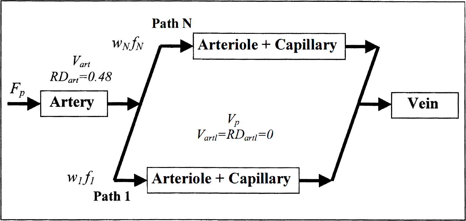
Vascular model. Flow is directed in multiple pathways, with w_i representing the fraction of flows with values f_i·Fp, where F_p is total flow. Tissue flow, F_p, feeding artery volume V_art, and tissue blood volume Vp were allowed to vary. The dispersion (RD_artl) and volume (V_artl) of arteriolar vascular elements in the original model of Kroll et al. (1996) were set to zero.

Flow heterogeneity from residue data

We used the fact that the impulse response to a plasma tracer can be estimated by nonparametric deconvolution of the tissue residue during the tracer passage by a noninvasively determined AIF. From this we derive the distribution of plasma transit times, and—under certain assumptions regarding the distribution of capillary lengths—the distribution of flows in the region.

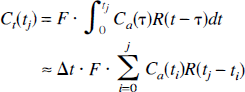
The tissue concentration C_t(t) of tracer in response to an arterial input function C_a(t) is given by

C_{t} (t) = F \cdot C_{a} (t) \otimes R (t) \equiv F \cdot \int_{0}^{t} C_{a} (τ) R (t - τ) d τ

(1)

where F is tissue flow and R is the residue function, i.e., the fraction of tracer present in the vasculature at time t after a perfect, infinitely sharp input in the feeding vessel. Assuming the arterial and cerebral concentrations are measured at equally spaced time-points t₁, t₂ = t_i + Δt, …, t_N, with Δt as the space between time points of measurement, this equation can be discretized, assuming that over short time intervals Δt, the residue function and arterial input values are constant in time:

\begin{matrix} C_{t} (t_{j}) = & F \cdot \int_{0}^{t_{j}} C_{a} (τ) R (t - τ) d t \\ \approx & Δ t \cdot F \cdot \sum_{i = 0}^{j} C_{a} (t_{i}) R (t_{j} - t_{i}) \end{matrix}

(2)

\begin{matrix} F \cdot Δ t \cdot & (\begin{matrix} C_{a} (t_{1}) & 0 & . . & 0 \\ C_{a} (t_{2}) & C_{a} (t_{1}) & . . & 0 \\ . . & . . & . . & . . \\ C_{a} (t_{N}) & C_{a} (t_{N - 1}) & . . & C_{a} (t_{1}) \end{matrix}) ∙ (\begin{matrix} R (t_{1} \\ R (t_{2}) \\ . . \\ R (t_{N}) \end{matrix}) \\ = & (\begin{matrix} C_{t} (t_{1} \\ C_{t} (t_{2}) \\ . . \\ C_{t} (t_{N}) \end{matrix}) \end{matrix}

(3)

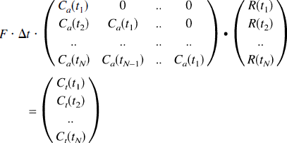
As previously described (Østergaard et al., 1996a), this equation can be modified to residue and arterial input functions that vary linearly in time. The SVD approach provides a powerful numerical tool to solve Eq. 3 in the presence of experimental noise to yield the residue function. The distribution of transit times, h(t), is then found from

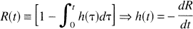
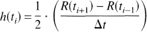
R (t) \equiv [1 - \int_{0}^{t} h (τ) d τ] \Rightarrow h (t) = - \frac{d R}{d t}

(4)

i.e., the slope of the residue function. We therefore estimated h(t) at a given time point t_i as

h (t_{i}) = \frac{1}{2} \cdot (\frac{R (t_{i + 1} - R (t_{i - 1})}{Δ t})

(5)

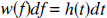
h(t) is turned into a distribution of relative flow rates f, w(f), by requiring

w (f) d f = h (t) d t

(6)

and, by the central volume theorem (Stewart, 1894),

f \cdot F = \frac{V}{t}

(7)

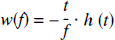
where V is the vascular volume. Assuming all vascular paths have equal volume, the distribution of flow rates is obtained by combining Eqs. 6 and 7:

w (f) = - \frac{t}{f} \cdot h (t)

(8)

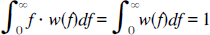
Finally, the distribution is normalized to have unit mean flow and area, i.e.,

\int_{0}^{\infty} f \cdot w (f) d f = \int_{0}^{\infty} w (f) d f = 1

(9)

MATERIALS AND METHODS

Volunteer data

Six healthy volunteers (age 29 ± 4 years) were examined according to our standard perfusion protocol on a GE Signa 1.5 T imager (General Electric, Waukesha, WI, U.S.A.) retrofitted for echo planar imaging capabilities (Instascan, Advanced NMR Systems, Wilmington, MA, U.S.A.), using spin echo, echo planar imaging with a time of repetition of 1.0 seconds, and a time of echo of 100 milliseconds. The slice thickness was 5 mm with an in-plane resolution of 1.6 mm by 1.6 mm in a 40 by 20 cm field-of-view. A total of 52 images were acquired, starting 15 seconds before intervenous injection of 0.3 mmol/kg contrast medium (Dysprosium-diamide, Nycomed Imaging, Oslo, Norway). Intravascular contrast agent concentrations, C(t), were estimated assuming a linear relationship between concentration and change in transverse relaxation rate, ΔR₂ (Villringer et al., 1988; Weisskoff et al., 1994):

C (t) \propto Δ R_{2} (t) = - l o g (\frac{S (t)}{S (0)}) / T E

(10)

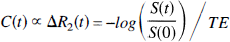
where S(0) and S(t) are the signal intensities at the baseline and at time t, respectively. Feeding arterial branches were identified in the image slice as pixels displaying early concentration increase after contrast injection (Porkka et al., 1991). This approach does not determine absolute arterial tracer levels, but provides the shape of the AIF. To standardize the analysis below, the arterial input function was therefore scaled to yield a mean cerebral blood volume of 3% (Østergaard et al., 1998a). In volunteers, a single arterial input function in the imaging plane was used for all tissue regions.

Determination of flow heterogeneity

Tissue concentration time curves were formed using Eq. 10. Three gray and two white matter tissue regions consisting of four image pixels (0.05 cm³) were then chosen, based on cerebral blood volume maps (Rosen et al., 1990, 1991a, b). The tissue residue function was calculated by SVD deconvolution of the tissue concentration time curve with the AIF. The resulting residue function was then converted into a PDF of relative flows as described in the Theory section above.

Model analysis

The experimentally determined flow heterogeneity PDF was then entered into the vascular model described above. For 16 gray and white matter regions (0.25 to 0.4 cm³), F_p, V_p, and V_art were adjusted to obtain optimal fits to the corresponding tissue concentration time curves by nonlinear regression analysis (Chan, 1993). The initial conditions were F_p = 40 mL/(100 mL·min), V_p = 2%, and V_art = 0.1%. The remaining model parameters are given in Fig. 1.

Comparison with model-free approach

To compare the flow rates obtained with the vascular model with those of the model-free SVD approach (Østergaard et al., 1996a, b), the height of the deconvolved tissue response curve (F_t·R(t_i) in Eq. 3), was determined for the same regions as used in the model analysis above. After determining mean white matter flow rate, nine relative gray-to-white flow ratios were calculated for each volunteer, and compared with those obtained by the vascular model.

Sensitivity to tracer delays

In volunteer 4, each pixel tissue concentration time curve was delayed in steps of 0.25 second by linear interpolation to simulate the effects of tracer arrival delays. The simulated image data were then analyzed as described above, and fitted flow rates by the SVD and vascular model approach plotted as a function of delay for comparison.

Sensitivity to noise and initial conditions

To determine the overall sensitivity of parameter estimates with the vascular model to experimental noise, a set of synthetic data sets were generated using the vascular model itself, and two sets of typical values for flow, volume, and feeding artery volume (F_p = 20 mL/(100 mL·min), V_p = 2%, V_art = 0.5%, and F_p = 50 mL/(100 mL/min), V_p = 3%, V_art = 0.5%). These were converted into a MR signal intensity time curve using Eq. 10, to generate a typical signal loss (25% for gray matter, equivalent to the higher flow) during a bolus passage. Random gaussian noise was then added, and “noisy” concentration time curves were again calculated from Eq. 10. Simulated signal-to-noise ratios (SNRs) varied from 400 to 12, the latter being typical for raw, pixel-by-pixel data obtained with our perfusion protocol on a clinical MR system. The synthetic curves were analyzed using the vascular model, using two different sets of initial conditions. These were chosen to represent two extremes of physiological values: F_p = 80 mL/(100 mL·min), V_p = 6%, V_art = 1%, and F_p = 20 mL/(100 mL·min, V_p = 2%, V_art = 0.1%. For each SNR, 24 simulations were performed, and the mean and standard deviations of the fitted model parameters were calculated for further evaluation. The dependency on initial conditions was evaluated by recording the number of simulations in which two different initial conditions caused resulting fitted parameters to differ by more than 10% from their mean. To compare stability of the vascular model and SVD method to experimental noise, flow rates were determined from the same synthetic curves by the SVD method.

RESULTS

Figure 2 shows a set of typical tissue and arterial concentration time curves obtained from volunteer 1. The tissue regions of interest consisted of 25 to 35 pixels (corresponding to 0.3–0.4 cm³ volumes). The average SNR (defined as the maximum tissue R2 increase during bolus passage divided by the standard deviation of the noise relative to prebolus base-line image intensity) for the tissue volumes used for model validation (0.25 to 0.4 cm³) was 30. The SNR of gray matter was a factor of 2 to 3 higher than that of white matter, due to the higher blood volume.

FIG. 2.

Typical tissue and arterial concentration time curves obtained from volunteer 1. Tissue volumes were roughly 0.3 cm³. The average signal-to-noise ratio (defined as the maximum tissue R₂ increase during bolus passage divided by the standard deviation of the noise relative to prebolus base-line image intensity) for the tissue volumes used for model validation (0.25 to 0.4 cm³) was 30.

Flow heterogeneity

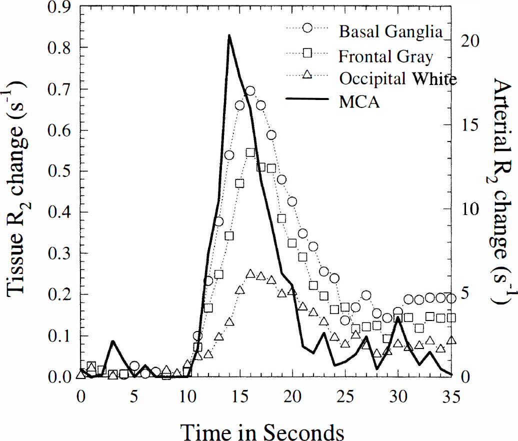
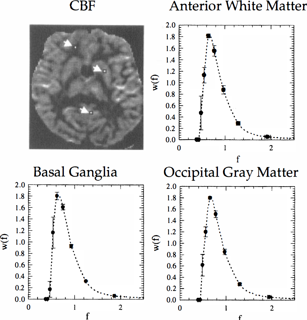
Figure 3 shows the location and size of three regions chosen for determination of flow heterogeneity in volunteer 4. The regions are overlaid on a CBF map calculated by the SVD-method to illustrate the contrast and spatial resolution of the techniques. Also shown are the corresponding flow heterogeneity plots derived from the three regions. The transit time and derived flow heterogeneity PDFs were found to be remarkably similar among regions and among volunteers. Figure 4A shows all pairs of relative transit time t and corresponding h(t) measured for all regions in all 6 volunteers. Figure 4B shows—under the assumption of equal capillary lengths—the corresponding plot of relative flow f and w(f) measured for all regions and volunteers. Because of this constancy across regions and subjects, the (f,w(f)) points were consequently averaged into 30 points (full curve) and used as a global expression for flow heterogeneity in normal tissue in the subsequent model analysis. The distribution of flows is markedly right-skewed, with the majority of capillaries having flow rates less than the mean flow. The maximum probability is reached at roughly two thirds of the mean flow.

FIG. 3.

Location of size of regions chosen for heterogeneity measurements overlaid onto a CBF map calculated by the singular value decomposition approach (volunteer 13). Also shown are the plots of heterogeneity probability density function for the corresponding regions. The symbols and error bars were derived as the mean and standard deviation of the values in the corresponding pixels (four pixels per region).

FIG. 4.

(A) shows a scatter-plot of all pairs of t (transit time relative to mean transit time) and h(t) determined in all regions of all volunteers. (B) shows the corresponding plot for f and w(f), measured for all regions and volunteers. The curves varied very little among tissue types and among volunteers. Consequently, the averaged w(f) curve was used as a global expression for flow heterogeneity in normal tissue in subsequent model analysis. The distribution of flows is markedly right-skewed, with the majority of capillaries having flow rates less than the mean flow. The maximum probability is reached at roughly two thirds of the mean flow. Notice a small population of very high flows.

Model validation

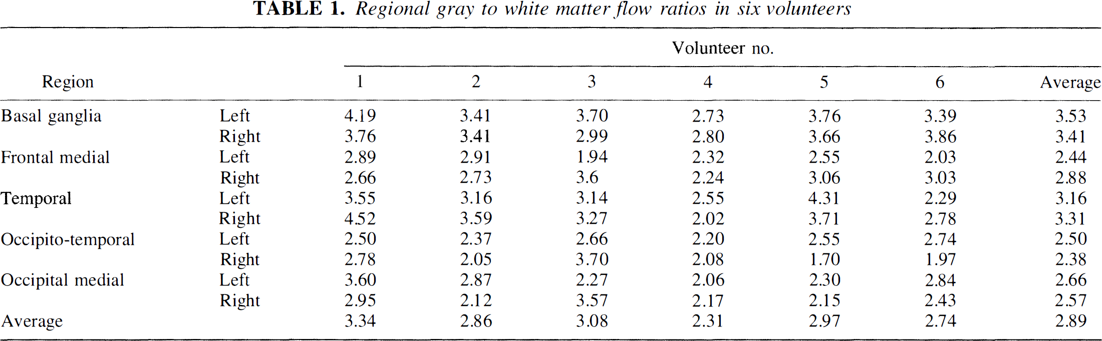
In the following, the experimentally determined flow heterogeneity PDF was applied, and the vascular transport is therefore described by only three parameters, V_art, F_p and V_p. Figure 5 shows a typical set of tissue concentration time curves as well as the fits provided by the model. Notice the model takes into account the observed earlier tracer arrival in tissue with higher flow rates. Also shown are the χ²-values for the fits. The quality of model fits to experimental data shown in Fig. 5 is typical for the patients examined. Table 1 shows the mean gray-to-white matter flow ratios for eight regions. The mean gray-to-white flow ratio was 2.89 ± 0.35 with the vascular model.

FIG. 5.

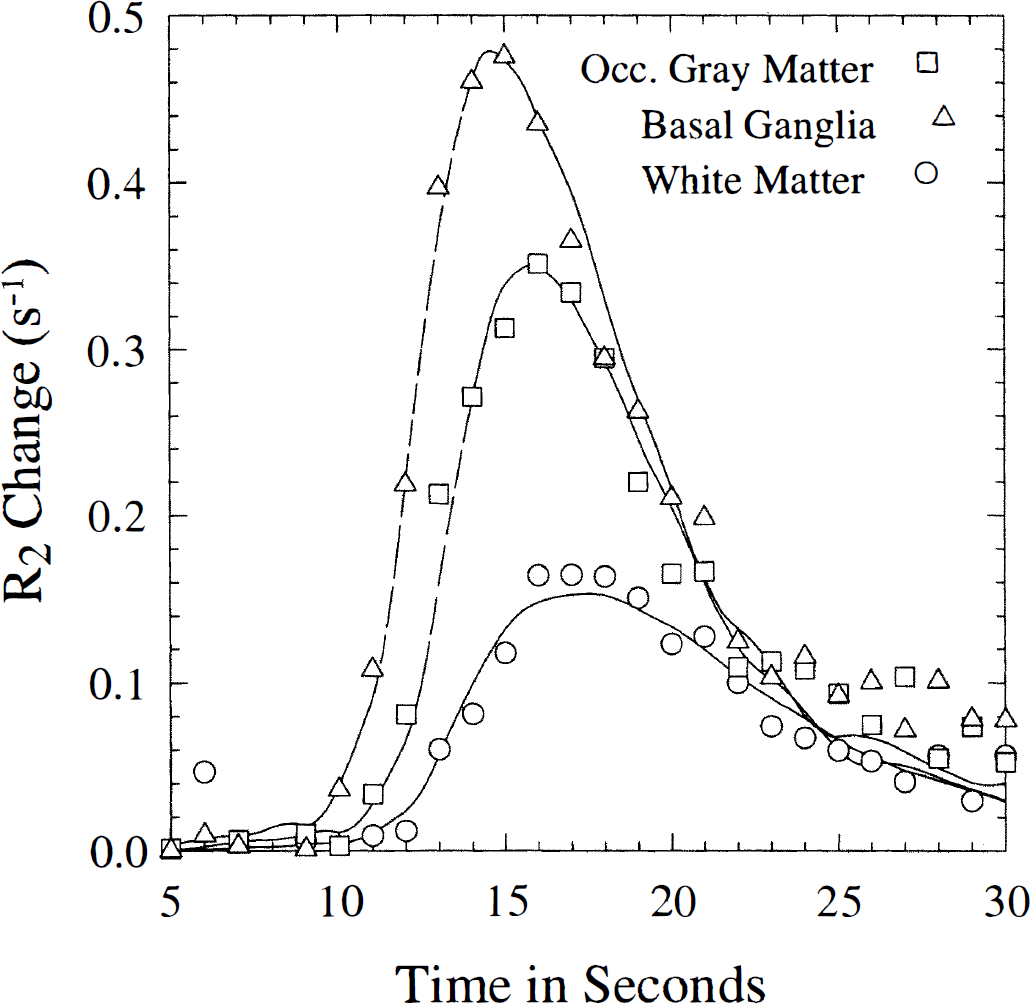
Typical tissue concentration time curves as well as the fits provided by the model. Basal ganglia: CBF = 60.3 ± 1.0 (SE) mL/(100 mL·min) (χ² = 51.0); gray matter: CBF = 48.5 ± 1.2 mL/(100 mL·min) (χ² = 54.5); white matter: CBF = 19.5 ± 0.8 mL(100 mL·min) (χ² = 24.6), In general, the model provided excellent fits to the experimental data. Data from volunteer 4. SE = standard error.

TABLE 1.

Regional gray to white matter flow ratios in six volunteers

		Volunteer no.
Region		1	2	3	4	5	6	Average
Basal ganglia	Left	4.19	3.41	3.70	2.73	3.76	3.39	3.53
	Right	3.76	3.41	2.99	2.80	3.66	3.86	3.41
Frontal medial	Left	2.89	2.91	1.94	2.32	2.55	2.03	2.44
	Right	2.66	2.73	3.6	2.24	3.06	3.03	2.88
Temporal	Left	3.55	3.16	3.14	2.55	4.31	2.29	3.16
	Right	4.52	3.59	3.27	2.02	3.71	2.78	3.31
Occipito-temporal	Left	2.50	2.37	2.66	2.20	2.55	2.74	2.50
	Right	2.78	2.05	3.70	2.08	1.70	1.97	2.38
Occipital medial	Left	3.60	2.87	2.27	2.06	2.30	2.84	2.66
	Right	2.95	2.12	3.57	2.17	2.15	2.43	2.57
Average		3.34	2.86	3.08	2.31	2.97	2.74	2.89

Comparison with model-free approach

Figure 6 shows gray-to-white matter flow ratios determined by the model approach plotted versus corresponding ratios in identical regions determined by the SVD approach. The three volunteers were chosen based on a significant spread in individual, regional gray-to-white matter ratios to facilitate comparison between approaches. In the figure, linear regression lines for each volunteer are shown. Notice regional gray-to-white matter ratios using the two techniques all lie near the line of identity.

FIG. 6.

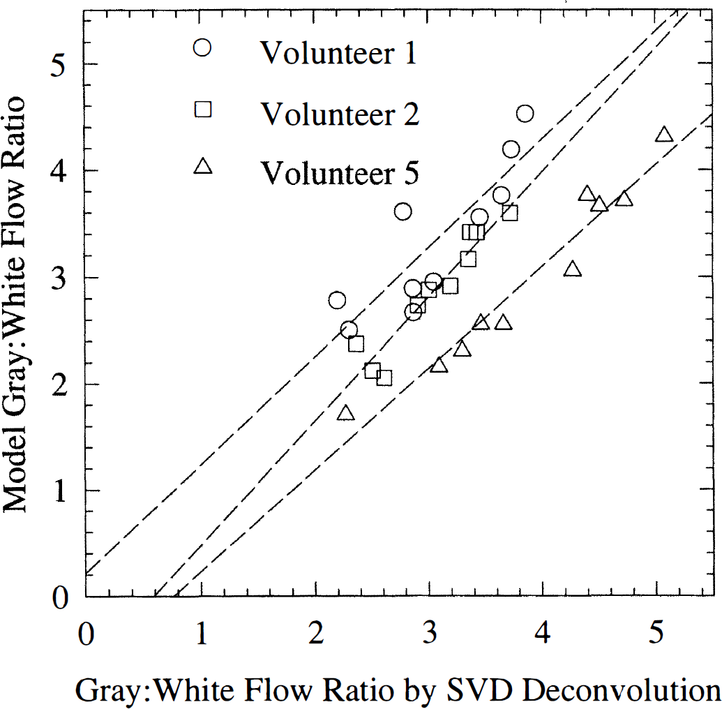
Model fits of regional gray-to-white matter flow ratios plotted versus those determined by the singular value decomposition (SVD) approach. Three volunteers were chosen based on a significant spread in their regional flow ratios (9 in each volunteer). Also shown are three linear regression lines, one for each of the volunteers ratios. Volunteer 1: y = 1.02 + 0.21 (r² = 0.75), volunteer 2: y = 1.16x −0.68 (r² = 0.91), volunteer 5: y = 0.95 × −0.72 (r² = 0.95). The line of identity was within the 95% confidence intervals of a common linear fit. Notice the agreement between gray-to-white flow ratios determined by the model and SVD approach, respectively.

Sensitivity to tracer arrival delays

Figure 7A shows the effect of AIF delay on fitted flow rates for the vascular model and the SVD approach, respectively. The gray and white matter tissue regions of interest consisted of 90 image pixels (1.1 cm³), Vascular model and SVD values were obtained from identical regions. The SVD approach progressively underestimates flow rates with tracer arrival delay. The relative underestimation is roughly proportional to the delay, reaching 25% for white matter and 35% for gray matter at a delay of 3 seconds, respectively. For the model approach, flow estimates are remarkably independent of delay. Figure 7B shows the fitted feeding artery volume as a function of delay. The model interprets increasing delays as increased feeding vessel volume in accordance with the definition of the vascular operator. Notice fluctuations of fitted flow values around 1 is accompanied by fluctuations of the fitted vascular volumes. These fluctuations and the tendency of flow and vascular volume to covary is discussed below.

FIG. 7.

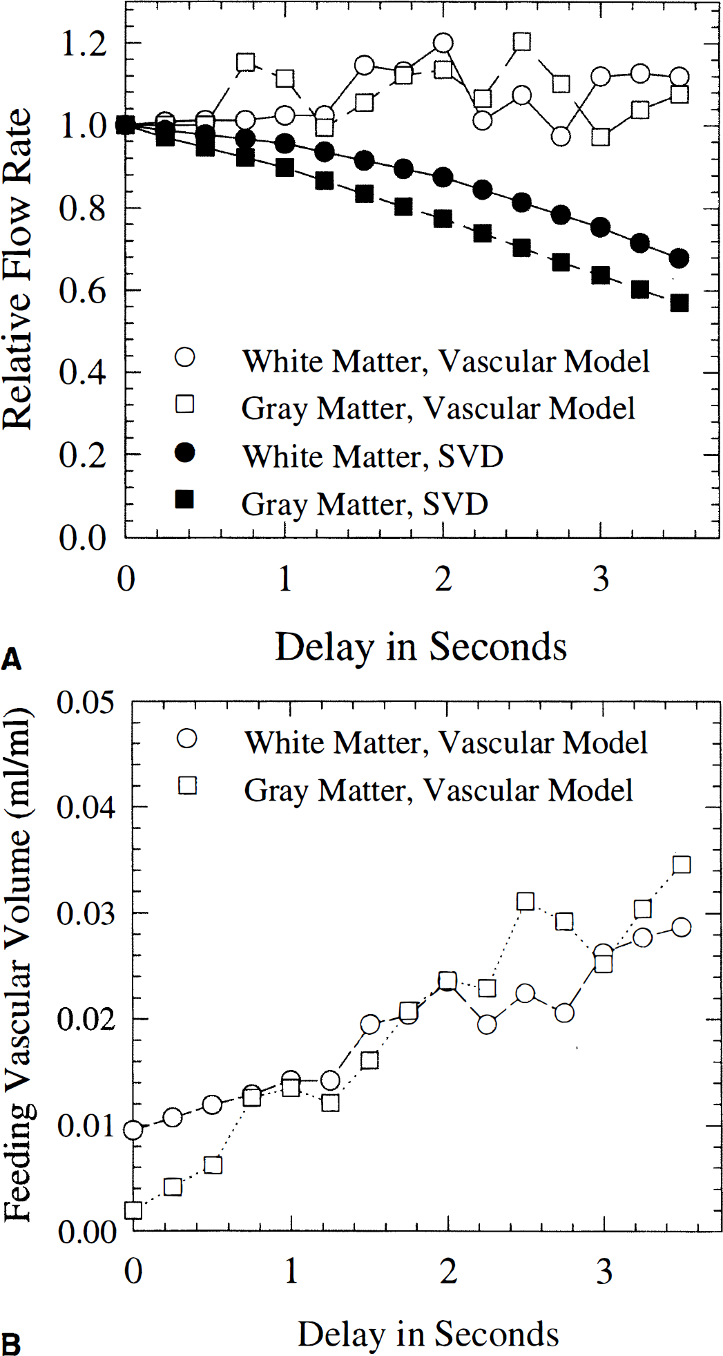
Effect of arterial input function delay on fitted flow rates for the vascular model and the singular value decomposition (SVD) approach, respectively (A). The gray and white matter tissue volumes were 0.8 cm³, and vascular model and SVD fits were obtained from identical regions. Figure 7B shows the fitted, feeding vessel volume (V_art) as a function of the delay. In accordance with the model, a delay is interpreted as a larger, feeding vessel volume. As vascular dispersion is a priori unknown in actual measurements, fitting was performed assuming a vascular dispersion RD_art = 0.48, although the delay was simulated to be dispersion-less. Notice deviations from exact linearity of the flow rates (A) were accompanied by similar deviations of the fitted feeding artery volume (B). Also, fitted flow rates fluctuated substantially around unit relative flow.

Sensitivity to noise and initial conditions

Figure 8 shows the means and standard deviations of the fitted flow rates for two sets of simulated data (V_art = 0.5%, F_p = 60 mL/(100 mL·min), V_p = 3%; V_art = 0.5%, F_p = 20 mL/(100 mL/min), V_p = 2%), using the model (Fig. 8A) and SVD (Fig. 8B) approach, respectively. The SVD approach overestimates flow rates somewhat for this choice of model parameters, whereas the vascular model fits are roughly equal to the input parameters. The uncertainty (error bars in Figs. 8A and 8B indicate one standard deviation, derived from the simulated data) on fitted flow rates display the expected increase as a function of increasing raw image data noise. For low SNR, error bars are roughly equal in size for the SVD and model approach, respectively. For high SNR, however, the uncertainty on vascular model fits did not reach zero as was the case for the SVD approach. To investigate whether factors other than noise contributed to the observed behavior, we analyzed the dependence of model fits on initial conditions and the tendency of parameters to covary. The fraction of fits, where initial conditions were found to significantly affect the fitted flow rates (defined as cases where two different initial conditions resulted in fitted flows that differed by more than 10% from their mean) was found to be negligible for SNR above 20. For lower SNR, 15% to 20% of fits gave ambiguous results. Therefore, the standard deviations for the low SNR may be somewhat underestimated due to bias by the choice of initial conditions.

FIG. 8.

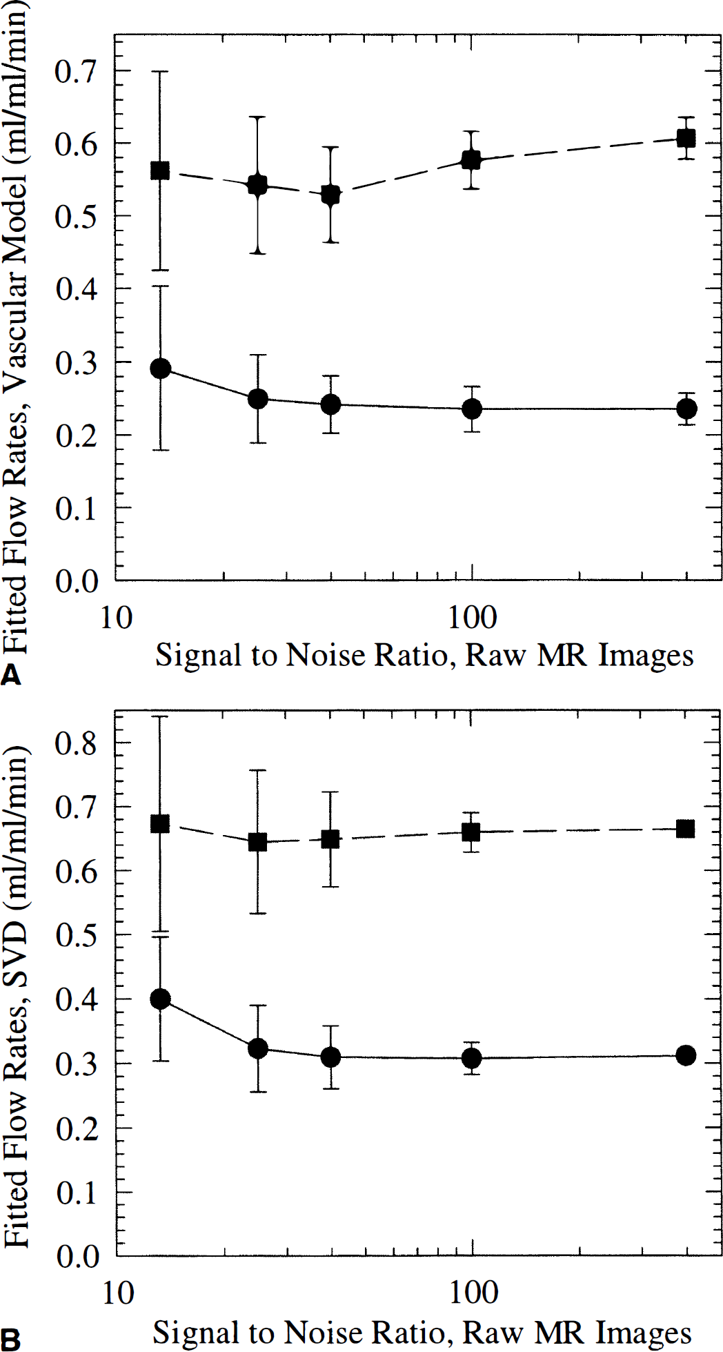
Means and standard deviations of fitted flow rates for two sets of simulated data (V_art = 0.5%, F_p = 60 mL/(100 mL·min), V_p = 3% and V_art = 0.5%, F_p = 20 mL/(100 mL·min), V_p = 2%). Raw image data noise was varied from that of typical, clinical data (~12) to 400.

During simulations, fitted feeding artery volumes and fitted tissue flows were found to covary: hence, high, fitted flow rates were often accompanied by high arterial volumes. Figure 9 shows fitted flow rates versus corresponding fitted feeding artery volumes from simulated curves with SNR = 40. This pattern of covarying fitted flow rates and feeding artery volumes was found at all noise levels. We found that varying flow and feeding artery volume in proportion lead to only small changes in the shape of the resulting concentration time curve. Therefore, the presence of modest experimental noise leads to relatively large uncertainties in fitted flow rates. This is thought to explain the unexpected, large standard deviation of flow estimates at high SNR for the vascular model, as well as the fluctuations around unit relative flow in Fig. 7.

FIG. 9.

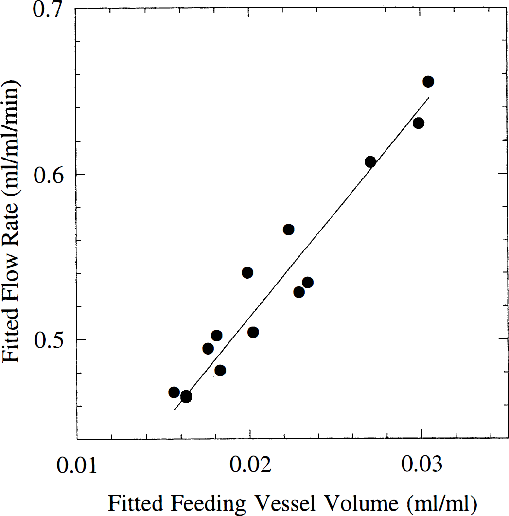
Fitted flow rates and arterial volumes (V_art) for signal-to-noise ratio (SNR) = 40. Input values were F_p = 50 mL/(100 mL·min) and V_art = 0.5%. Notice curves with large, but proportional deviations of flow and volume from the “true” values fitted simulated concentration time curves at even this relatively high SNR.

DISCUSSION

Overall validity of model

The vascular model, after incorporation of the experimentally determined heterogeneity PDF, provided excellent fits to the experimental data. The model fits of CBF yielded a mean gray-to-white flow ratio of 2.8 ± 0.35, in agreement with the PET literature ratio of 2.65 for subjects of similar age (Leenders et al., 1990). The ratios were also in good agreement with those found using the model-free approach. In contrast to the SVD approach, the model approach provided fits to experimental data that were essentially independent of vascular delay. The model was simplified considerably by the use of one flow heterogeneity PDF for all types of tissue. By characterizing the model by only three parameters, we obtained a remarkable stability of the model, even compared to the pixel-by-pixel based SVD approach. Covarying vascular volume and flow rate in model fits to low SNR data was found to be a major contributor to uncertainty in model fits of CBF. Below, we will discuss the individual elements of the model in further detail.

Model considerations

The model presented here differs slightly from that previously described by Kroll et al. (1996) for the heart. Kroll et al. (1996) described the arteriolar and capillary compartments separately, assigning fixed relative dispersion and variable volumes to the arteriolar vascular paths, and a fixed volume to the capillary bed. In the brain, capillary density varies greatly among different tissue types. For the purpose of obtaining a robust model for all types of brain tissue with the same choice of basic model parameters, we kept microvascular volume as a free parameter. In terms of vascular transport, the models are similar, except that in our model, dispersion takes place only in the large vessel, whereas small vessel dispersion is accounted for by the flow heterogeneity PDF. Despite the simplification of the model, we feel that, by limiting the number of vascular elements and thereby the number of free parameters, we may have contributed significantly to the stability of the model to noise as outlined in the analysis above. The robustness of the model to experimental noise is imperative to ultimately study CBF at high spatial resolution. Kroll et al. (1996) assumed that only small vessel tracer levels are observed by the residue detection. In our case, this assumption is further justified by the inherent sensitivity of susceptibility contrast to microvessels (Fisel et al., 1991; Weisskoff et al., 1994; Boxerman et al., 1995).

Vascular transport and dispersion term

As discussed elsewhere (Østergaard et al., 1996b), nonparametric deconvolution approaches do not allow separation of macrovascular transport and microvascular retention. Therefore, modeling vascular retention is necessary, whenever vascular transport significantly changes the input bolus shape upstream of the AIF measurement site. The vascular transport operator model used in the present model is generally accepted for modeling normal major vessel transport. The advantage of including vascular transport in the kinetic modeling is shown in Fig. 5: the fact that tracer arrives earlier in tissue with high flow rate because of a faster feeding vessel transit is accounted for by the model approach, unlike the model-free SVD approach. The difficulty in introducing this operator lies mainly in the fact that the transfer functions of the major vessel and the microvascular network are very similar. This, in turn, leads to the difficulty in separating feeding vascular volume and tissue flow, as observed in our simulations. Our analysis also suggest that this effect contributes significantly to the uncertainty of flow estimates by the vascular model, even at modest noise levels, just as it may play a role in the dependency upon initial conditions of fitted flow rates. These findings are in agreement with those previously reported by Kroll et al., (1996). In cerebrovascular diseases, blood may pass through stenoses with marked turbulence, or through irregular collateral paths upstream of the arterial sampling site. In these cases, the vascular operator may not be adequate, and the vascular transport function should ideally be measured independently. Indeed, novel MR techniques detecting the inflow of spin labeled arterial blood to a given brain region may ultimately provide this information (Wong et al., 1997). Such independent measurements would serve to avoid the interdependence of flow and vascular volumes using vascular models, or alternatively allow application of the model-free SVD approach. In severe cases, however, vascular dispersion may dominate total tracer retention, in which case estimates of flow rate by residue detection of an intravascular tracer become uncertain (Østergaard et al., 1996b; Kroll et al., 1996).

Flow heterogeneity

Reports of cerebral flow heterogeneity are mainly based on invasive measurements of plasma or red blood cell velocities in rats. Abounader et al. (1995) used bolus injection of a plasma marker followed by decapitation, deriving plasma flow velocity from capillary filling in histology. Hudetz et al. (1997) determined the frequency of red blood cell velocities in capillaries using intravital video microscopy. Both found the distribution of blood elements to be very heterogeneous, with a right-skewed shape. Figure 10 shows their findings along with our experimental PDF. The data of Hudetz et al. (1997) were normalized as our relative flow PDF (See Theory, Eq. 9). From the data of Abounader et al. (1995), a normocapnic data set was chosen, and axes scaled to facilitate comparison with the other curves (plasma flow units did not allow direct normalization). It should be noticed that these measurements are not directly comparable. First, plasma and red blood cells follow different paths through the capillary network, so our measurements should be more comparable to the plasma velocity measurements. Secondly, our flow distribution curve assumes equal capillary lengths. Although the relationship between capillary plasma flow and flow velocity is a complex function of capillary length and architecture, a finite distribution of capillary lengths is likely to result in blood velocities being more dispersed than relative capillary flows (as seen when comparing our PDF with the red blood cell velocity study). We feel the similarity of our measurements with these independent, invasive methods lends hope to the use of this approach in describing normal microvascular dynamics. In altered physiological states or disease, the flow heterogeneity may not be as constant among tissue types as found in this study. Abounader et al. (1995) determined the heterogeneity of micro vascular flow at different degrees of hypercapnia, and found that plasma flow became more homogenous at higher flows. A similar finding for red blood cell velocities was reported by Hudetz et al. (1997). This could be the case in disease as well, and caution should therefore be exercised in choosing flow heterogeneity PDF for use with vascular models in these cases. The model-free approach to determine flow heterogeneity PDF presented here may provide insight with respect to the distribution of relative flows in these cases. Using this approach, it should be kept in mind solving Eq. 1 belongs to a class of so-called inverse problem, meaning that any noise in measured tissue concentrations may lead to large changes in the resulting residue function. As suppression of noise inevitably causes loss of underlying information, the SVD deconvolution therefore may not yield the exact shape of the underlying residue function, Likewise, one may not be able to distinguish slightly different flow heterogeneity PDF based on noisy measured concentration time curves. Although the flow heterogeneity PDF and derived flow rates were found in agreement with independent findings, it is therefore important to further validate our approach.

FIG. 10.

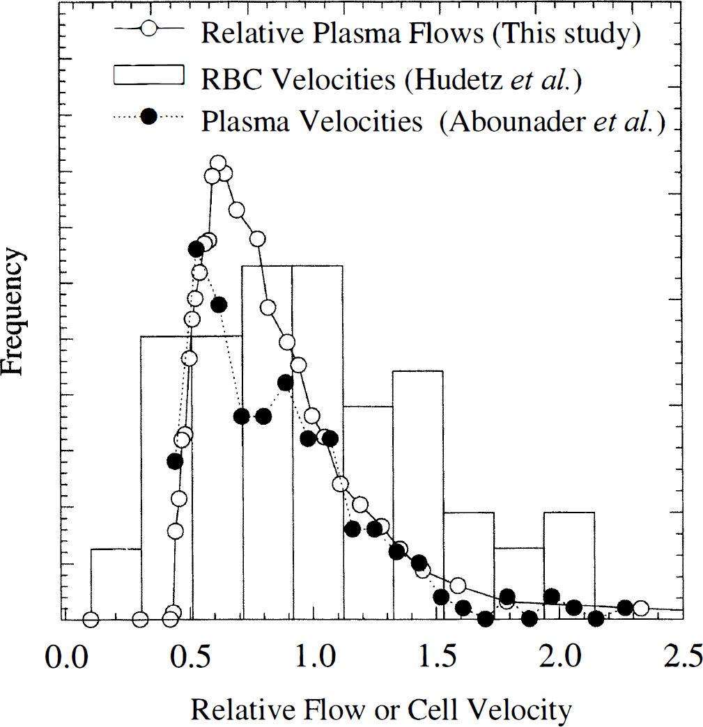
Distribution of plasma velocities (arbitrary units) in a normocapnic rat from Abounader et al. (1995), and red blood cell velocities measured by Hudetz et al. (1997). Also shown is our experimental flow probability density function. Notice all curves are very heterogeneous and right-skewed shape. Red blood cell velocities were normalized to allow direct comparison, whereas the plasma velocity units were measured in indirect units that did not allow normalization. Instead, axes were scaled to allow visual comparison.

Utility of vascular models

Although CBF itself is an important index of brain function, the heterogeneity of microvascular flow and transit times described here may be a more important determinant of cerebral metabolism. As discussed by Kuschinsky et al. (1992), the degree of heterogeneity among capillary paths determines the net capillary-to-tissue concentration gradients necessary to drive delivery of nutrients. Indeed, regulation of capillary flow heterogeneity may play a major role in the ability of the brain to increase, for example, oxygen delivery to meet cellular metabolic demands (Kuschinsky et al., 1992). This issue can be addresses in great detail by combining flow heterogeneity measurements with spatially distributed models of oxygen exchange (Li et al., 1997). The analysis presented here, combined with these models, may ultimately lead to a more extensive understanding of, for example, the fundamental limitations of oxygen delivery in stroke, where the survival of tissue may partially depend on the ability to increase oxygen extraction by an altered distribution of mean transit times. Also, modeling the exact relationship between cellular oxygen consumption and vascular oxygen levels may facilitate a quantitative metabolic interpretation of deoxyhemoglobin concentration changes observed by functional magnetic resonance imaging (Kwong et al., 1992).

Footnotes

Acknowledgments

The authors thank Prof. Wolfgang Kuschinsky, PhD, for helpful comments and for providing data for , and Dr. Brad Buchbinder, MD, for helping to acquire volunteer data. The authors are greatly indebted to the work and simulation tools of The National Simulation Resource (NIH RR-01243). Contrast agent for the study was kindly provided by Nycomed Imaging, Oslo, Norway.

Abbreviations used

References

Abounader

Vogel

Kuschinsky

(1995) Patterns of capillary plasma perfusion in brains in conscious rats during normocapnia and hypercapnia. Circ Res 76:120–126

Boxerman

Hamberg

Rosen

Weisskoff

(1995) MR contrast due to intravascular magnetic susceptibility perturbations. Magn Reson Med 34:555–566

Chan

Goldstein

Bassingthwaighte

(1993) SENSOP: a derivative-free solver for nonlinear least squares with sensitivity scaling. Ann Biomed Eng 21:621–631

Fisel

Ackerman

Buxton

Garrido

Belliveau

Rosen

Brady

(1991) MR contrast due to microscopically heterogeneous magnetic susceptibility: numerical simulations and applications to cerebral physiology. Magn Reson Med 17:336–347

Hudetz

Biswal

Feher

Kampine

(1997) Effects of hypoxia and hypercapnia on capillary flow velocity in the rat cerebral cortex. Microvasc Res 54:35–42

King

Deussen

Raymond

Bassingthwaighte

(1993) A vascular transport operator. Am J Physiol 265:H2196–H2208

King

Raymond

Bassingthwaighte

(1996) Modeling blood flow heterogeneity. Ann Biomed Eng 24:352–372

Kroll

Wilke

Jerosch

Wang

Zhang

Bache

Bassingthwaighte

(1996) Modeling regional myocardial flows from residue functions of an intravascular indicator. Am J Physiol 271:H1643–H1655

Kwong

Belliveau

Chesler

Goldberg

Weisskoff

Poncelet

Kennedy

Hoppel

Cohen

Turner

(1992) Dynamic magnetic resonance imaging of human brain activity during primary sensory stimulation. Proc Natl Acad Sci USA 89:5675–5679

10.

Kuschinsky

Paulson

(1992) Capillary circulation in the brain. Cerebrovasc Brain Metab Rev 4:261–286

11.

Leenders

Perani

Lammertsma

Heather

Buckingham

Healy

Gibbs

Wise

Hatazawa

Herold

(1990) Cerebral blood flow, blood volume and oxygen utilization. Normal values and effect of age. Brain 113:27–47

12.

Yipintsoi

Bassingthwaighte

(1997) Nonlinear model for capillary-tissue oxygen transport and metabolism. Ann Biomed Eng 25:604–619

13.

Østergaard

Johannsen

Poulsen

Vestergaard-Poulsen

Asboe

Gee

Hansen

Cold

Gjedde

Gyldensted

(1998b) Cerebral blood flow measurements by MRI bolus tracking: comparison with [150]H₂O PET in humans. J Cereb Blood Flow Metab 18:935–940

14.

Østergaard

Smith

Vestergaard-Poulsen

Hansen

Gee

Gjedde

Gyldensted

(1998a) Absolute cerebral blood flow and blood volume measured by MRI bolus tracking: comparison with PET values. J Cereb Blood Flow Metab 18:425–432

15.

Østergaard

Sorensen

Kwong

Weisskoff

Gyldensted

Rosen

(1996a) High resolution measurement of cerebral blood flow using intravascular tracer bolus passages. Part II: Experimental comparison and preliminary results. Magn Reson Med 36:726–736

16.

Østergaard

Weisskoff

Chesler

Gyldensted

Rosen

(1996b) High resolution measurement of cerebral blood flow using intravascular tracer bolus passages. Part I: Mathematical approach and statistical analysis. Magn Reson Med 36:715–725

17.

Porkka

Neuder

Hunter

Weisskoff

Belliveau

Rosen

(1991) Arterial Input Function Measurement with MRI. In: Proc Society Magnetic Resonance in Medicine, 10th Annual Meeting, San Francisco, 1991. p 120

18.

Rosen BR, Belliveau JW, Aronen HJ, Kennedy D, Buchbinder BR, Fischman A, Gruber M, Glas J, Weisskoff RM, Cohen MS, and others (1991a) Susceptibility contrast imaging of cerebral blood volume: human experience. Magn Reson Med 22:293–299

19.

Rosen BR, Belliveau JW, Buchbinder BR, McKinstry RC, Porkka LM, Kennedy DN, Neuder MS, Fisel CR, Aronen HJ, Kwong KK, and others (1991b) Contrast agents and cerebral hemodynamics. Magn Reson Med 19:285–292

20.

Rosen

Belliveau

Vevea

Brady

(1990) Perfusion imaging with NMR contrast agents. Magn Reson Med 14:249–265

21.

Stewart

(1894) Researches on the circulation time in organs and on the influences which affect it. Parts I-III. J Physiol (London) 15:1–45

22.

Villringer

Rosen

Belliveau

Ackerman

Lauffer

Buxton

Chao

Wedeen

Brady

(1988) Dynamic imaging with lanthanide chelates in normal brain: contrast due to magnetic susceptibility effects. Magn Reson Med 6:164–174

23.

Weisskoff

Zuo

Boxerman

Rosen

(1994) Microscopic susceptibility variation and transverse relaxation: theory and experiment. Magn Reson Med 31:601–610

24.

Wilke N, Kroll K, Merkle H, Wang Y, Ishibashi Y, Xu Y, Zhang J, Jerosch HM, Muhler A, Stillman AE, and others (1995) Regional myocardial blood volume and flow: first-pass MR imaging with polylysine-Gd-DTPA. J Magn Reson Imaging 5:227–237

25.

Wong

Buxton

Frank

(1997) Implementation of quantitative perfusion imaging techniques for functional brain mapping using pulsed arterial spin labeling. NMR Biomed 10:237–249

Modeling Cerebral Blood Flow and Flow Heterogeneity from Magnetic Resonance Residue Data

Abstract

Keywords

THEORY

Vascular model

Flow heterogeneity from residue data

MATERIALS AND METHODS

Volunteer data

Determination of flow heterogeneity

Model analysis

Comparison with model-free approach

Sensitivity to tracer delays

Sensitivity to noise and initial conditions

RESULTS

Flow heterogeneity

Model validation

Comparison with model-free approach

Sensitivity to tracer arrival delays

Sensitivity to noise and initial conditions

DISCUSSION

Overall validity of model

Model considerations

Vascular transport and dispersion term

Flow heterogeneity

Utility of vascular models

Footnotes

Acknowledgments

Abbreviations used

References