Sage Journals: Discover world-class research

Abstract

Several algorithms have been proposed to improve positron emission tomography quantification by combining anatomical and functional information in a pixel-by-pixel correction scheme. The precision of these methods when applied to real data depends on the precision of the manifold correction steps, such as full-width half-maximum modeling, magnetic resonance imaging-positron emission tomography registration, tissue segmentation, or background activity estimation. A good understanding of the influence of these parameters thus is critical to the effective use of the algorithms. In the current article, the authors present a monodimensional model that allows a simple theoretical and experimental evaluation of correction imprecision. The authors then assess correction robustness in three dimensions with computer simulations, and evaluate the validity of regional SD as a correction performance criterion.

Keywords

Positron emission tomography Partial volume effect correction Constrained image restoration Data fusion Gray matter positron emission tomography

A major limitation of positron emission tomography (PET) is the finite spatial resolution of PET scanners, Activity concentration is systematically underestimated or overestimated in objects smaller than two to three times the full-width at half-maximum (FWHM) of the device point spread function (PSF). Indeed, because of image smoothing by the device PSF, the activity in a structure partly spreads into the nearby tissues (“spill-out” effect), whereas the neighborhood activity partly contributes to the structure measurement (“spill-in” effect), This so-called partial volume effect (PVE) is globally characterized by the recovery coefficient, defined as the ratio of the measured over the true activity concentration (Hoffman et al., 1979; Mazziotta et al., 1981; Kessler et al., 1984; Bendriem et al., 1991; Kuwert et al., 1993).

Several algorithms have been proposed for restoring the images on a pixel-by-pixel basis. Because of the ill-conditioned nature of the restoration problem, some sort of regularization must be used to avoid high-frequency noise amplification (Natterer, 1988; Haber et al., 1990; Links et al., 1992; Chan et al., 1997). With the increasing resolution of computed tomography and magnetic resonance imaging (MRI), a family of algorithms has been proposed, where regularization is achieved by incorporating anatomical information and tissue homogeneity constraints in a noniterative pixel-by-pixel correction scheme. These algorithms include the binary atrophy correction (Videen et al., 1988; Meltzer et al., 1990), the gray matter (GM-PET) method (Müller-Gärtner et al., 1992), and the four-tissue correction (Meltzer et al., 1996). In this report, we refer to these algorithms as the anatomically guided pixel-by-pixel algorithms (APA).

Since they were first proposed, the APA have generated an increasing interest, and several improvements or variants have been published (Kosugi et al., 1996; Labbé et al., 1996; Knorr et al., 1997). However, the imprecision of the APA preprocessings, such as MRI segmentation or MRI-PET registration, significantly affect the corrected image and may make correction reliability questionable (Fahey et al., 1996; Strul and Bendriem, 1996; Yang et al., 1996; Meltzer et al., 1997).

This article addresses several issues of APA correction robustness. We first briefly formulate the overall mathematical frame of APA correction and show the main sources of instability. We then present a monodimensional model, which allows a simple theoretical and experimental evaluation of correction imprecision. Correction robustness in three dimensions then is assessed with computer simulations. Finally, we examine the usefulness and the limitations of regional SD as a criterion for GM-PET correction performance.

THEORY

The anatomically guided pixel-by-pixel algorithm correction formulas

In APA correction, an anatomical image (from MRI or computed tomography) is subdivided by segmentation into several tissue classes, which do not need to be either contiguous or homogeneous. For each tissue, a separate distribution image is derived from the segmented image, with values of 1 in all the pixels that belong to the tissue, and 0 everywhere else. The APA correction restores the true pixel-by-pixel activity concentration A_TT for one tissue only, named here the target tissue (TT). The other classes, for which no restoration is performed, are termed neighbor tissues (NT). Each NT is assumed to be homogeneous, with a mean activity concentration ${\overset{ˉ}{A}}_{N T}$ .

The observed image I_obs is written as the sum of all the tissue contributions, where each tissue contributes according to its activity concentration and to its distribution function:

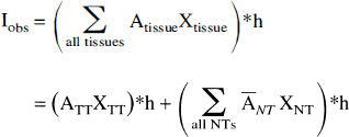
\begin{aligned} I_{o b s} & = (\sum_{a l l t i s s u e s} A_{t i s s u e} X_{t i s s u e}) * h \\ = (A_{T T} X_{T T}) * h + (\sum_{a l l N T s} {\bar{A}}_{N T} X_{N T}) * h \end{aligned}

(1)

where * signs the convolution operator and “h” is the PET image PSF.

The APA correction assumes that the TT is at least approximately homogeneous (Müller-Gärtner et al., 1992), so that

(A_{T T} X_{T T}) * h ≅ A_{T T} (X_{T T} * h)

(2)

A corrected estimation C_TT of the activity concentration A_TT is obtained by combining equations (1) and (2):

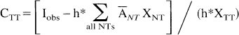
C_{T T} = [I_{o b s} - h * \sum_{a l l N T s} {\bar{A}}_{N T} X_{N T}] / (h * X_{T T})

(3)

This correction can be understood as a two-step restoration process. First, the spill-in from the NT is subtracted from the TT measurement. Second, the 1/(X_TT*h) term acts as an amplification coefficient, which compensates for the loss resulting from the partial spill-out of TT activity to the NT. The correction must be limited to areas where (X_TT*h) is much greater than zero, to minimize noise amplification.

The first APA procedure was the binary atrophy correction, which relied on only one radioactive compartment, comprising all of the brain tissue voxels (Videen et al., 1988; Meltzer et al., 1990):

C_{b r a i n t i s s u e} = I_{o b s} / (h * X_{b r a i n t i s s u e})

(4)

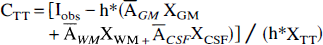
The GM-PET algorithm improves correction by separating white matter (WM), GM, and CSF (Müller-Gärtner et al., 1992):

C_{G M} = [I_{o b s} - h * ({\bar{A}}_{W M} X_{W M} + {\bar{A}}_{C S F} X_{C S F})] / (h * X_{G M})

(5)

The four-tissue correction is a two-step extension of GM-PET (Meltzer et al., 1996). The image is first corrected using GM-PET equation, then a focal hypoactive or hyperactive GM area is set apart from the rest of the GM as a specific TT:

\begin{aligned} C_{T T} = & [I_{o b s} - h * ({\bar{A}}_{G M} X_{G M} \\ + {\bar{A}}_{W M} X_{W M +} {\bar{A}}_{C S F} X_{C S F})] / (h * X_{T T}) \end{aligned}

(6)

Factors of correction instability

Equation (3) shows that APA corrections strongly depend on the precision of all processing steps: segmentation of the anatomical image, anatomical-functional registration, sampling rate conversion, measurement of the NT mean activity concentration, and evaluation of the PSF. The limited precision of most of these procedures may lead to significant correction instability. For example, the measurement of the mean activity concentrations in the NT often is biased by the TT spill-out and scattering, especially when NT-TT contrast is important. The precision of the tissue segmentation also is limited by instrumental artefacts and by classification problems affecting mixed voxels. The accuracy of the PSF model generally is limited by the neglect of resolution nonuniformity or scattering to shorten computation time. Last, unless specially designed head holders and protocols are used, the limited precision of current registration techniques further limits correction robustness.

The APA corrections depend on numerous parameters, and an exhaustive study of APA precision would lead to complicated equations. Thus, we address this issue using a simplified monodimensional model, valid both for GM-PET and binary corrections, which allows us to reduce the number of free parameters. To keep generality, we make assumptions only on the tissue maps used for correction, with absolutely no assumption on the real tissue map. This independence is necessary to treat binary correction, where the binary tissue map used for correction neglects the WM-GM separation.

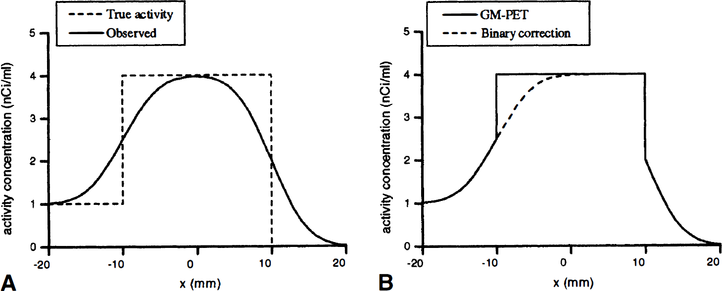
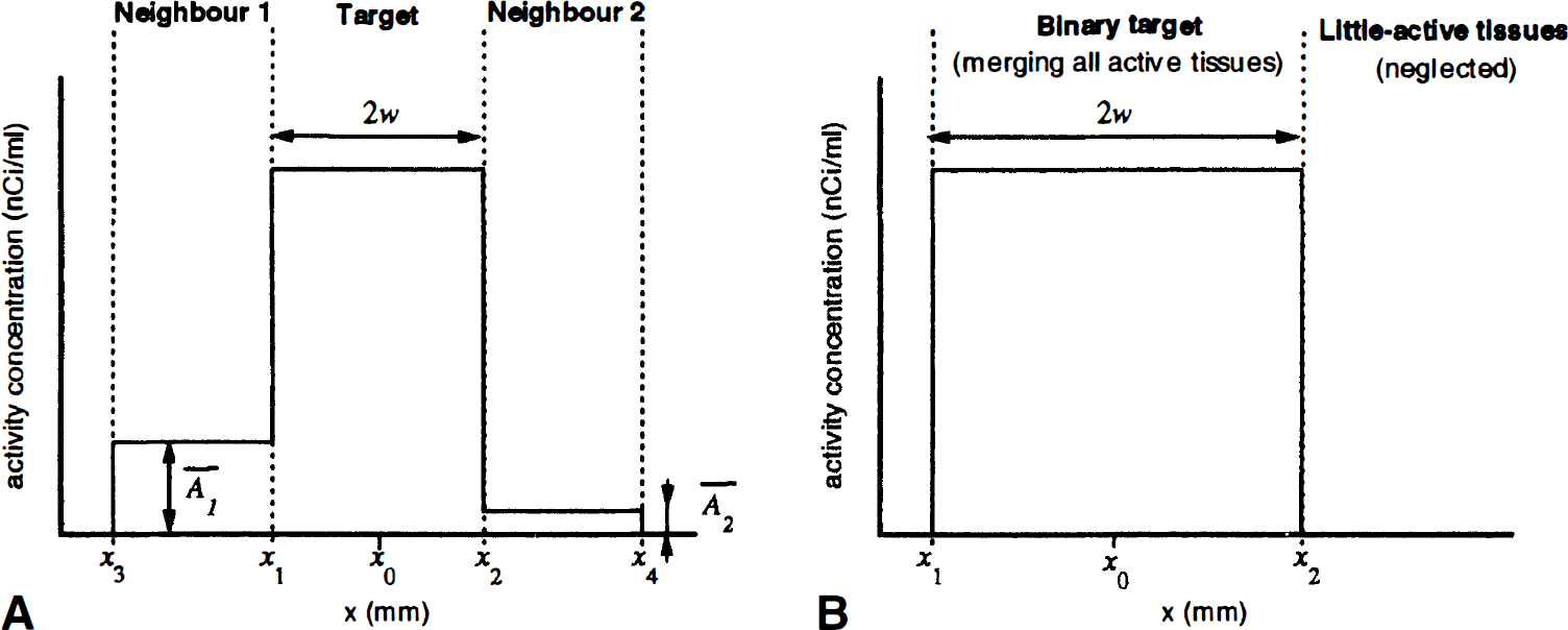
The parameters used for APA correction are assumed to follow the model presented on Fig. 1A. The segmented TT is an active bar, of center x₀ and half-width w, thus extending between two locations x₁ = x₀ – w and x₂ = x₀ + w. It is inserted between two NT, NT₁ (activity concentration ${\overset{ˉ}{A}}_{1}$ , ranging from x₃ to x₁) and NT₂ (activity concentration ${\overset{ˉ}{A}}_{2}$ , ranging from x₂ to x₄). The PSF used for correction is a normalized Gaussian function, whose width is specified by its SD (σ), with FWHM = 2.35*σ.

FIG. 1.

Monodimensional model. (A) General case (like gray matter-positron emission tomography [GM-PET]). The target tissue (TT) is inserted between two neighbor tissues (NT). The influence of the tissues outside of the range x₃ to x₄ is assumed to be negligible around the TT (e.g., they are not active or they are distant from more than 3 full-width at half-maximum [FWHM]). (B) Special case corresponding to binary correction: the NT are either neglected like NT₂ or included in the target tissue like NT₁.

This model is approximately met in various common situations, such as GM-PET correction of a small cortex area or an internal GM nucleus, where the NT may be WM and CSF, respectively, or both WM. No distant NT is taken into account in this model for reasons of simplicity, but the equations presented later are easily extended to an arbitrary number of NT. The model may be further simplified if the outer NT boundaries are distant from TT (a few FWHM values are enough) by setting x₃ ≈ –∞ and x₄ ≈ +∞. This model also may apply to binary correction by merging all of the active tissues (Fig. 1B).

If we neglect the uncertainty on NT segmentation, the correction now depends on only five parameter estimations: the activity concentrations ${\overset{ˉ}{A}}_{1}$ and ${\overset{ˉ}{A}}_{2}$ (if there are any), the PSF SD σ, the TT center location x₀ (obtained by registration) and the TT half-width w (obtained by segmentation). Thus, by neglecting interparameter correlations, and by assuming the parameter imprecision to be small, we can write:

\begin{aligned} v a r [C_{T T}] = & {(\frac{\partial C_{T T}}{\partial {\bar{A}}_{1}})}^{2} v a r [{\bar{A}}_{1}] + {(\frac{\partial C_{T T}}{\partial {\bar{A}}_{2}})}^{2} v a r [{\bar{A}}_{2}] \\ + {(\frac{\partial C_{T T}}{\partial x_{0}})}^{2} v a r [x_{0}] + {(\frac{\partial C_{T T}}{\partial w})}^{2} v a r [w] \end{aligned}

(7)

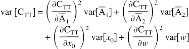
This equation expresses the relationship between the precision of the APA parameters and the statistical precision of the corrected image. This statistic is not directly connected to image noise but rather to correction reproducibility: in any point where var[C_TT] is high, APA correction may yield different values from one correction process to another. For noisy images, another term should be added, corresponding to the image noise amplification by APA correction. Since correction FWHM is initially fixed by the user and then used for all corrections, FWHM errors tend to introduce systematic rather than random errors. Then, it was not included in equation (7) but was investigated as a bias later in this report.

The expressions of the partial derivatives needed for computation of the correction variance are summarized below (see appendix for details of the derivation):

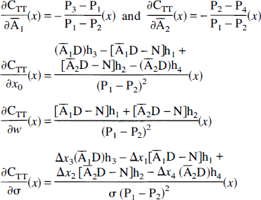
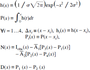
\begin{aligned} \frac{\partial C_{T T}}{\partial {\bar{A}}_{1}} (x) = - \frac{P_{3} - P_{1}}{P_{1} - P_{2}} (x) a n d \frac{\partial C_{T T}}{\partial {\bar{A}}_{2}} (x) = - \frac{P_{2} - P_{4}}{P_{1} - P_{2}} (x) \\ \frac{\partial C_{T T}}{\partial x_{0}} (x) = \frac{\binom{({\bar{A}}_{1} D) h_{3} - [{\bar{A}}_{1} D - N] h_{1} +}{[{\bar{A}}_{2} D - N] h_{2} - ({\bar{A}}_{2} D) h_{4}}}{(P_{1} - P_{2})^{2}} (x) \\ \frac{\partial C_{T T}}{\partial w} (x) = \frac{[{\bar{A}}_{1} D - N] h_{1} + [{\bar{A}}_{2} D - N] h_{2}}{(P_{1} - P_{2})^{2}} (x) \\ \frac{\partial C_{T T}}{\partial σ} (x) = \frac{\binom{Δ x_{3} ({\bar{A}}_{1} D) h_{3} - Δ x_{1} [{\bar{A}}_{1} D - N] h_{1} +}{Δ x_{2} [{\bar{A}}_{2} D - N] h_{2} - Δ x_{4} ({\bar{A}}_{2} D) h_{4}}}{σ (P_{1} - P_{2})^{2}} (x) \end{aligned}

(8)

where we use the following notations:

\begin{aligned} h (x) \equiv (1 / σ \sqrt{2 π}) \exp (- x^{2} / 2 σ^{2}) \\ P (x) \equiv \int_{0}^{x} h (t) d t \\ \forall i = 1 \dots 4, Δ x_{i} \equiv (x - x_{i}), h_{i} (x) \equiv h (x - x_{i}), \\ P_{i} (x) \equiv P (x - x_{i}), \\ N (x) \equiv I_{o b s} (x) - {\bar{A}}_{1} [P_{3} (x) - P_{1} (x)] \\ - {\bar{A}}_{2} [P_{2} (x) - P_{4} (x)] \\ D (x) \equiv P_{1} (x) - P_{2} (x) \end{aligned}

(9)

These equations are first-order approximations of the actual error and variance functions and are thus limited to small errors. Within their field of validity, these equations might provide a foundation for the analysis of APA correction errors and imprecision. In the following text, their characteristic shapes are exemplified, and assessed by comparison with computer simulations.

Quality criteria

The correction robustness is crucial for the effective use of APA algorithms. Brain PET imaging often is used to discriminate between several groups of subjects such as controls and patients. If the correction performances differ greatly from one subject to another, the results of the comparison may be affected and thus misleading. In this regard, as is pointed out by several authors, absolute quantification is less important than comparison significance (Di Chiro and Brooks, 1988; Strother et al., 1991; Kuwert et al., 1993). Thus, the correction errors introduced earlier could be a major limitation to the practical use of APA corrections.

Given the complexity of MRI-PET registration and MRI segmentation, improving correction robustness might be difficult. It may then be more relevant to define correction quality criteria. Ideally, such criteria would reveal erroneous corrections and help determine the cause of the error. Correction parameters then could be fixed, in a manual or automatic manner, to improve data processing.

As shown later, correction errors can lead to large artefacts, which severely decrease regional homogeneity in the corrected areas with regard to error-free correction. This then suggests homogeneity as one possible criterion. In the material that follows, we assess the quality of one criterion measuring homogeneity, the regional SD, to bring into evidence both the utility and the limitations of this approach.

MATERIALS AND METHODS

Monodimensional bar experiment

The APA correction artefacts and variance were explored in the monodimensional case. A model consistent with the correction of a short brain profile around the cortex was considered (Fig. 2A). The NT₁, corresponding to the WM, was assumed to be wide enough to be approximated as semi-infinite (x₃ was rejected toward –∞) to simplify the analysis of the correction artefacts. To be consistent with the hypotheses commonly used in GM-PET correction, the NT₂ (corresponding to the CSF and bone) was assumed inactive and thus was neglected. The cortex was assumed to be 20-mm wide, and the contrast between cortex and WM was set to 4: I. Simulations were performed according to the following equation (centered on the middle of the cortex):

I_{o b s} (x) = {\bar{A}}_{G M} [P_{1} (x) - P_{2} (x)] + {\bar{A}}_{l} [1 / 2 + P_{1} (x)]

(10)

with ${\overset{ˉ}{A}}_{G M}$ = 4 nCi · mL⁻¹, ${\overset{ˉ}{A}}_{1}$ = 1 nCi · mL⁻¹, w = 10 mm, x₀ = 0 mm, and FWHM = 9 mm.

FIG. 2.

Model used for the one-dimensional experiment. (A) True and observed activity distributions. This model is similar to the one presented on Fig. 1 A, with NT₁ semi-infinite (x₃ rejected toward –∞) and NT₂ neglected. (B) Optimal GM-PET and binary corrections.

Both binary and GM-PET corrections were applied following equations (4) and (5) (detailed in equations [15] and [21] of the appendix). The tissue distribution used for GM-PET correction was the same as the one used for simulation, with the TT being the cortex. For binary correction, the binary tissue map was obtained by merging the NT₁ and the cortex maps (thus rejecting x₁ toward –∞. Various processing errors were introduced in both corrections: inaccurate NT activity concentration estimates, incorrect FWHM, segmentation errors, and registration errors, and the corrected image profiles were compared with those predicted by equation (8).

The pixel-by-pixel corrected activity expectation and SD were computed by performing 10,000 correction tries in presence of random parameter errors, extracted from Gaussian distributions, with SD[ ${\overset{ˉ}{A}}_{1}$ ] = 0.2 nCi · mL⁻¹, SD[x₀] = 1 mm, and SD[w] = 1 mm. The experimental SD profiles were compared with those predicted by equation (7).

Implementation of anatomically guided pixel-by-pixel algorithm correction

For the following experiments, we used a C implementation of APA correction, which accepts any number of tissue classes for noniterative processing. The correction PSF is the product of a transaxial and an axial Gaussian functions. Sampling rate conversion is achieved by trilinearly downsampling the tissue images after PSF blurring. The correction mask is automatically created by downsampling the original TT tissue map, then thresholding the result-image at 0.5 to avoid large correction amplification.

Simulation library

We used a simulation library in which any digital phantom model is defined as a combination (addition, subtraction, or embedding) of simple radioactive geometrical shapes, or primitives. The corresponding model activity function and primitive distribution functions are sampled on a high-resolution image grid to compute the activity concentration image and the primitive distribution images, respectively. A PET simulation is derived from the activity concentration image using a convolution-downsampling scheme: the activity image is first convolved with the PSF model, then downsampled to the sampling characteristics of typical PET images. Measurement volumes of interest (VOI) are computed for any primitive by downsampling its distribution image, then thresholding the result, with threshold = 0.5.

Quantitative analysis

For the sphere experiments described later, all measurements were performed inside six VOI covering the whole spheres. Quantitative accuracy was measured by computing the VOI regional bias, equal to the difference between the measured and the real activity concentrations inside the VOI.

To evaluate the quantitation recovery performed by APA correction, a performance index, the bias reduction coefficient (BRC), was defined as follows:

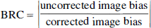
B R C = | \frac{u n c o r r e c t e d i m a g e b i a s}{c o r r e c t e d i m a g e b i a s} |

(11)

The BRC index is used to determine whether APA correction has improved or worsened PVE errors. Large BRC values (>1) show excellent quantitative recoveries. On the contrary, a BRC lower than 1 indicates that APA correction has increased the image bias.

As mentioned previously, we also measured the regional image SD, computed for each VOI as follows:

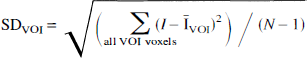
{S D}_{V O I} = \sqrt{(\sum_{a l l V O I v o x e l s} (I - {\bar{I}}_{V O I})^{2}) / (N - 1)}

(12)

where N is the number of voxels in the VOI, and I and ${\overset{ˉ}{I}}_{V O I}$ are the activity concentration observed in each voxel and in the VOI (mean value), respectively.

Digital sphere phantom experiment

A digital model from a Data Spectrum Sphere phantom (Data Spectrum Corp., Chapel Hill, NC, U.S.A.) was modeled (Fig. 3). The model comprised six hot spheres (diameters = 9.5, 12.7, 15.9, 19.1, 25.4, and 31.9 mm, respectively; activity = 1000 nCi/mL) embedded in a warm cylinder (diameter = 200 mm, activity = 250 nCi/mL). We used this model to produce high-definition activity images (256*256* 128 voxels, voxel dimensions = 1* 1* 1 mm). We then derived low-definition simulations from the activity images. The characteristics of these simulations were chosen to be similar to those of ECAT 953/31B images (128*128*31 voxels, voxel dimensions = 1.995* 1.995*3.375 mm, transaxial FWHM = 9 mm, axial FWHM = 5 mm). We also derived six low-definition VOI from the model, with the downsampling-thresholding scheme described previously, each fully covering one sphere. We investigated the quantitative influence on GM-PET correction of four error factors.

FIG. 3.

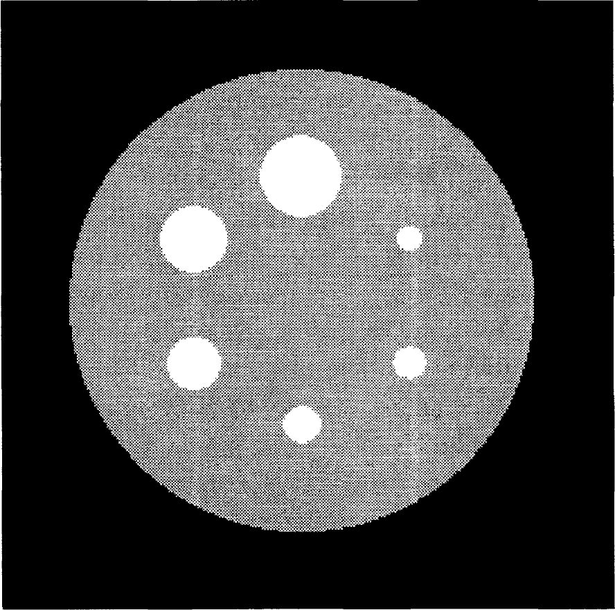
The digital sphere phantom (medium slice).

Influence of the neighbor tissue activity concentration measurement. We introduced inaccurate measurements of cylinder activity concentration in APA correction, modulating the error from −50% to +50% of the true value (i.e., 125 to 375 nCi/mL).

Influence of the modeling. Similarly, we used inaccurate transaxial FWHM for correction, with error ranging from −30% (FWHM = 6 mm) to +30% (FWHM = 12 mm) of the true FWHM.

Influence of magnetic resonance imaging-positron emission tomography registration. We first computed the PET simulation using the true phantom model, then displaced it (from −5 to +5 mm by steps of 0.5 mm), and used the mispositioned model to produce the tissue images used in the APA algorithm and to produce the measurement VOL We chose this procedure to reproduce the current image analysis, in which VOI are drawn on the anatomical images.

Influence of segmentation threshold. Since the most commonly used segmentation approaches rely on the determination of classification thresholds, the modification of these thresholds leads to displacements of tissue boundaries. To assess the influence of these global displacements, we added a fixed value (from −1.25 to + 1.25 mm) to each sphere radius after simulation. We then derived the tissue images and the measurement VOI from the modified model, as was done in the previous investigation.

RESULTS

Monodimensional experiment

The corrected activity profiles are plotted on Fig. 2B. For the GM-PET correction, the correct activity concentration is fully recovered within the correction mask (the GM area), whereas no correction is performed outside this mask. For the binary correction, since the binary tissue map merges the NT₁ and the GM, only the x₂ edge is corrected for PVE.

Profiles of the derivatives of C_TT(x), as recovered with GM-PET method, are plotted on Fig. 4. They should be understood as follows: when a partial derivative is positive, any overestimation of the corresponding parameter yields a positive artefact, and parameter underestimation leads to a negative artefact. The direction of the artefacts is inverted for negative partial derivatives. Notice that, in the conditions that were chosen for computation, 1 nCi·mL⁻¹ corresponds to a 25% error, with regard to the true GM activity concentration.

FIG. 4.

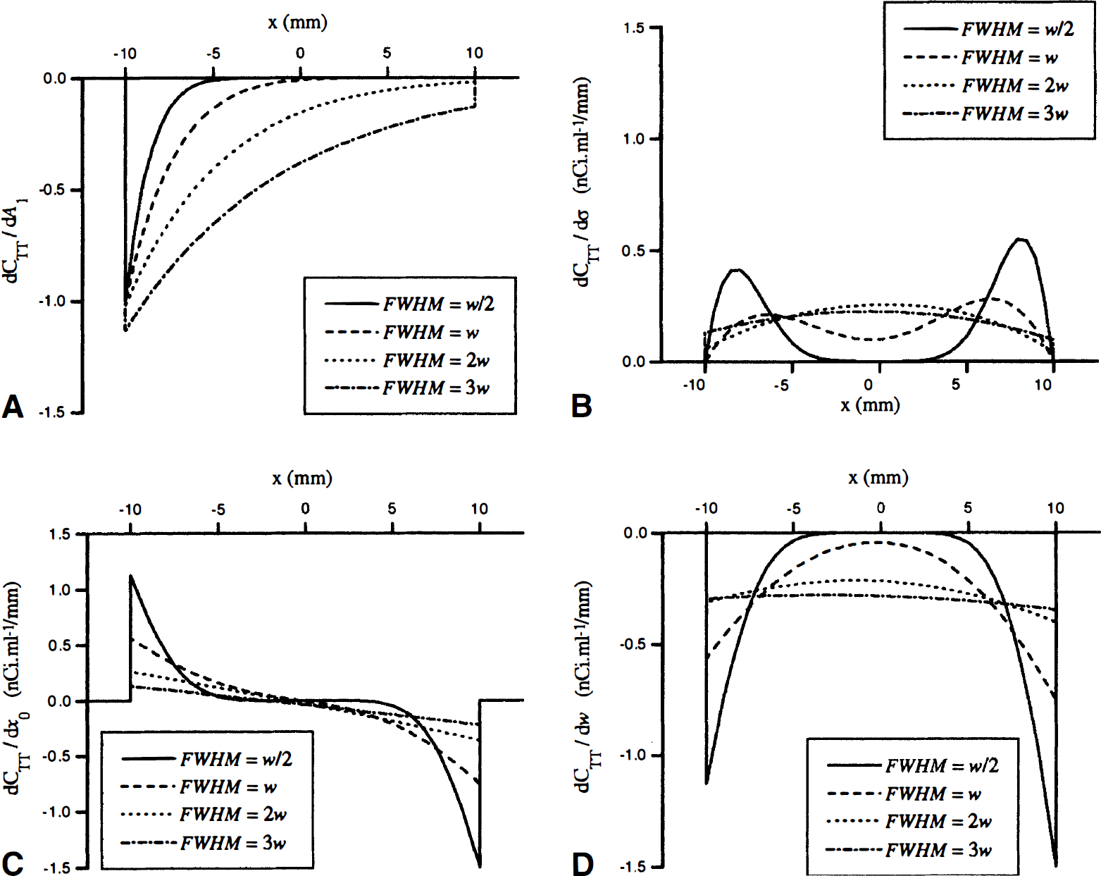
Theoretical GM-PET partial derivatives profiles for the one-dimensional experiment model at various resolutions. (A) Derivative relative to At activity estimation. (B) Derivative relative to errors on the resolution SD. (C) Derivative relative to registration errors. (D) Derivative relative to segmentation errors. The derivatives are written in (nCi·mL⁻¹) of corrected activity per (nCi·mL⁻¹) of NT activity on (A), and in (nCi·mL⁻¹) of corrected activity variation per millimeter of parameter variation everywhere else. Computations performed with ${\overset{ˉ}{A}}_{G M}$ = 4 nCi·mL⁻¹, A, = 1 nCi·mL⁻¹, w = 10 mm.

AH correction artefacts appear as error functions propagating from the TT edges toward the center. The errors thus are maximum near the TT edges, except for FWHM mismatches (Fig. 4B). In the latter case, each edge-error function reaches its maximum (for small FWHM) only at a distance from the edges nearly equal to the PSF SD σ. For all errors, the correction artefacts vanish at a distance (roughly 3 σ from the TT edges. The ratio between the structure width and the FWHM thus is critical: when the structure is overly small, the edge artefacts tend to cover the whole structure, leading to a global increase of the correction error. For FWHM, segmentation, and registration errors, the contrast is critical, too, with the artefacts on Fig. 4B to D being distinctly smaller on the x₁ edge than on the opposite one.

The segmentation and registration errors share the same basic artefact pattern, corresponding to the error induced by the shift in the positions of the TT map boundaries x₁ and x₂ (Fig. 4C and D). In qualitative terms, there is a negative artefact wherever the correction TT map overlaps the NT, and there is a positive artefact wherever the correction TT map does not reach the real TT boundary. Strikingly, the error magnitude on the TT edges increases rapidly as the FWHM decreases. Indeed, approximating the earlier equation for small FWHM shows that the maximum error is inversely proportional to the FWHM.

Figure 5 displays some typical GM-PET correction artefacts. The dashed lines represent the theoretical predictions derived from equation (8). The agreement is excellent for NT activity or FWHM errors (Fig. 5A and B). For registration and segmentation errors (Fig. 5C and D), discrepancies appear, with the positive artefacts being larger than the negative ones. Figure 5E and F exemplifies some combinations of segmentation and registration errors: they compensate each other on one TT edge and are added on the opposite edge, leading to strong artefacts on this edge.

FIG. 5.

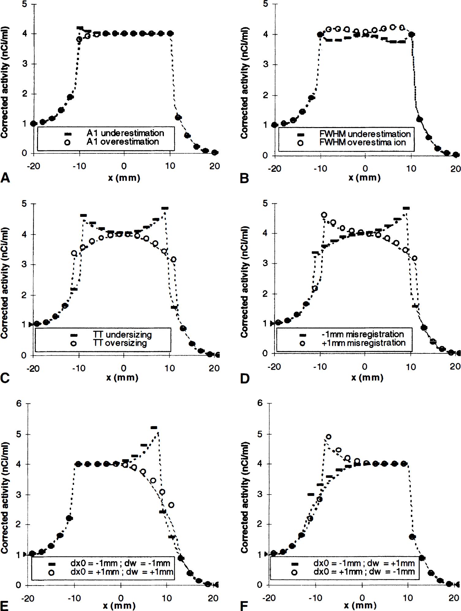
Correction artefacts in GM-PET method. (A) Inaccurate estimation of white matter activity concentration (±0.2 nCi·mL⁻¹). (B) Inaccurate FWHM estimation (±2 mm). (C) Missegmentation errors (±1 mm on each TT edge). (D) Misregistration errors (±1 mm). (E) Combination of missegmentation and misregistration errors, both + 1 mm or both −1 mm. (F) Combination of opposite missegmentation and misregistration errors. The dotted lines represent the theoretical predictions.

Similar artefact patterns appear for binary correction, but only near the outer edge (Fig. 6). Since the x₁ edge of the binary map is neglected in this model, registration and segmentation errors lead to identical artefacts (Fig. 6B and C), which may as well combine in addition (Fig. 6D) or in subtraction. Notice that binary correction always neglects the activity of the tissues located outside of the brain. If this assumption was erroneous, a small edge artefact would appear (symmetrical to the one presented on Fig. 5A) and would combine with any other correction error.

FIG. 6.

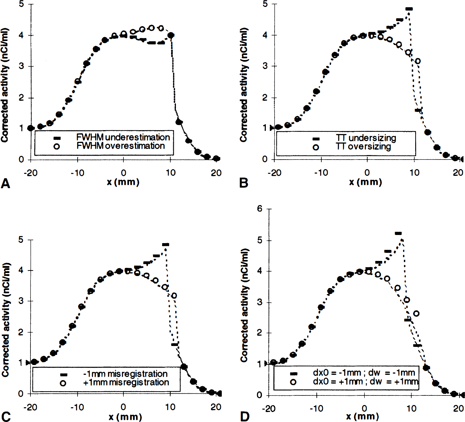
Correction artefacts in binary correction. (A) Inaccurate FWHM estimation (±2 mm). (B) Missegmentation errors (± 1 mm on each TT edge). (C) Misregistration errors (±1 mm). (D) Combination of missegmentation and misregistration errors, both + 1 mm or both −1 mm. The dotted lines represent the theoretical predictions.

Figure 7 compares the measured pixel-by-pixel corrected activity SD with theoretical predictions. The agreement is perfect when correction imprecision comes from NT activity estimation imprecision (Fig. 7A). For identical registration and segmentation imprecisions, the profiles are identical, and we have plotted only the registration profiles. When the correction mask is ideally located (matching the real TT), the measured imprecision is only slightly superior to the theoretical one (Fig. 7B). In real conditions, the correction mask is affected in size and position by the registration and segmentation errors. The experimental SD profile then is distinctly different from the theoretical one (Fig. 7C), being both lower and wider. If registration imprecision is increased to 2 mm, or if l-mm registration and segmentation imprecisions are combined, the discrepancy is more noticeable (Fig. 7D), the experimental imprecisions being substantially lower than the predicted values.

FIG. 7.

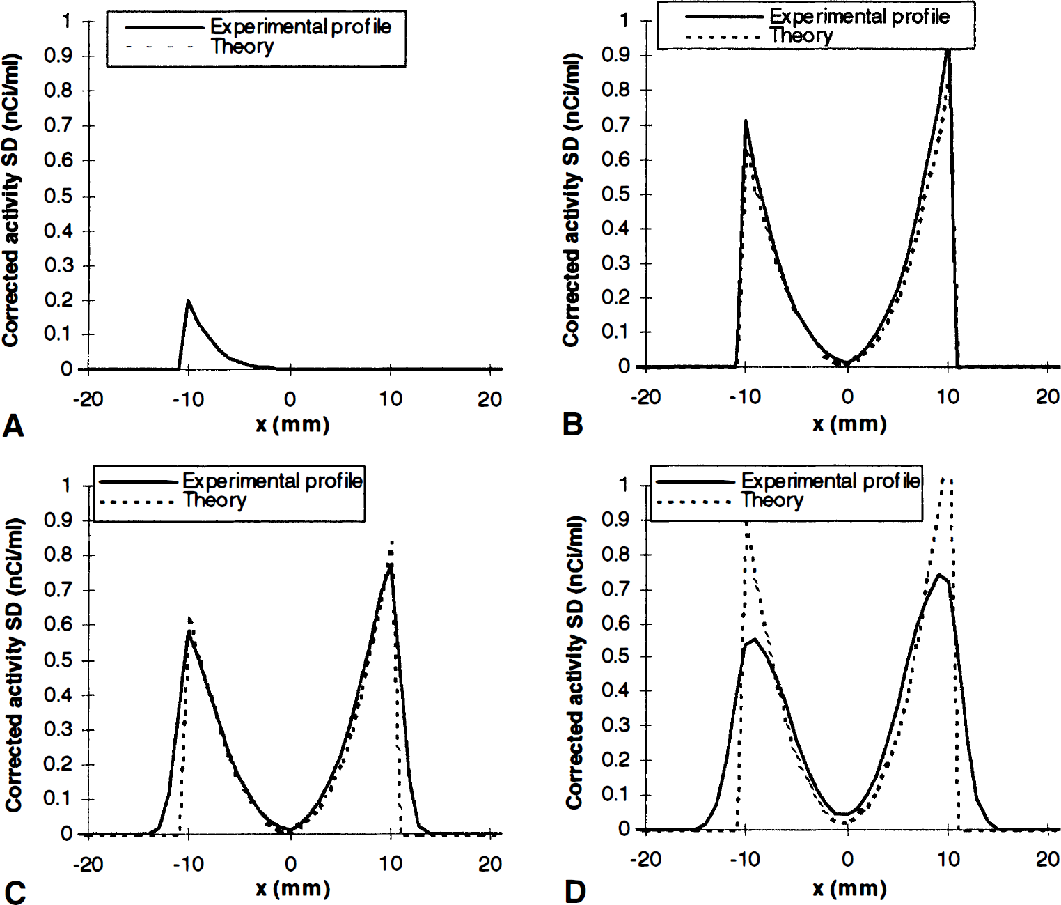
Correction precision in GM-PET method, measured by corrected activity SD. (A) With SD[ ${\overset{ˉ}{A}}_{1}$ ] = 0.2 nCi·mL⁻¹. (B) With SD[x₀] = 1 mm and ideal correction mask. (C) With SD[x₀] = 1 mm and correction mask in real conditions. (D) With SD[w] = SD[x₀] = 1 mm and correction mask in real conditions.

The influence of the correction mask results from the asymmetry between inward TT edge-shifts, which exclude the edge points from correction, and outward TT edge-shifts, which induce undercorrection errors. In both cases, the corrected activity is lowered compared with the true activity. Consequently, the imprecision is lowered, but at the price of a negative statistical bias (Fig 8A). When the correction mask is fixed, there is a positive statistical bias, since positive registration or segmentation artefacts are globally higher than negative ones (Fig. 8B).

FIG. 8.

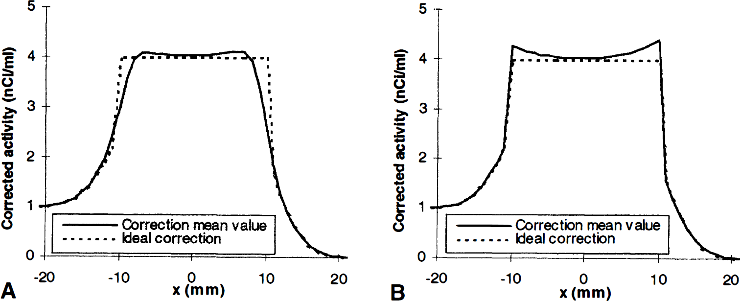
Mean corrected activity profile (10,000 tries) in presence of segmentation and registration imprecision (SD[w] = SD[x₀] = 1 mm). (A) With correction mask in real conditions. (B) With ideal correction mask.

Digital sphere phantom

Figure 9 displays the performance of GM-PET correction for each sphere. When it was possible, the data have been fitted with empirical models (first- or second-degree polynomials and their inverse functions), and missing BRC values were extrapolated.

FIG. 9.

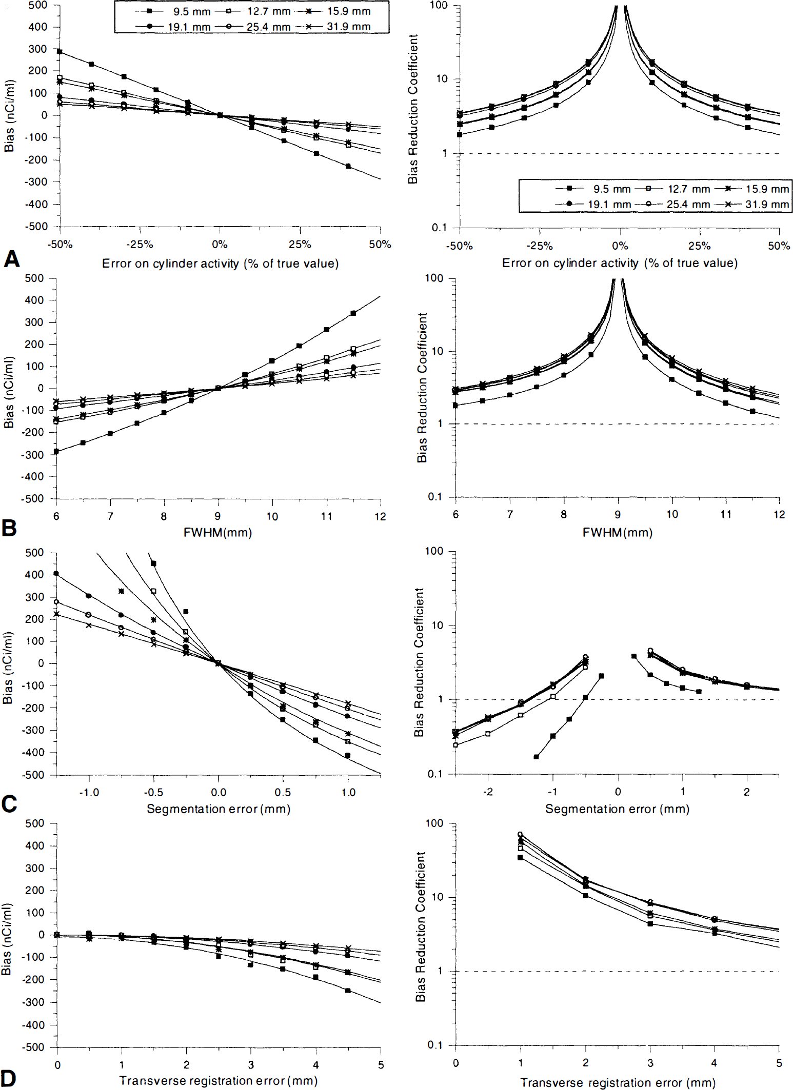
Influence of the processing errors on the corrected image regional bias (left) and BRC (right) for each sphere. (A) white matter activity estimation. (B) Correction FWHM. (C) Segmentation errors (error on sphere radii). (D) Registration.

Correction instability is greater for the smallest spheres. In presence of registration and segmentation errors, this trend is amplified by their influence on the correction masks. Segmentation is the most critical factor contributing to the imprecision of correction, with the maximum bias (+2350 nCi/mL) appearing for the 1.25mm undersizing of the smallest sphere. The influence of sphere oversizing is less dramatic (maximum bias: −480 nCi/mL), and is comparable with FWHM overestimation (maximum bias: +420 nCi/mL). Maximum biases are lower for errors induced by incorrect WM activity concentration values or by misregistrations (290 and −190 nCi/mL, respectively). The BRC plots show that GM-PET correction usually improves quantification (BRC above 1). The sole exception occurred during sphere undersizing, where GM-PET correction degraded the regional bias (BRC less than 1) when the segmentation errors are larger than 0.75 mm.

Table 1 summarizes results extracted from these data. For the smallest sphere, a moderate error of cylinder activity or FWHM can result in a significant corrected image bias (–115 nCi/mL). The bias induced by a typical registration error is smaller (corrected image bias = −55 nCi/mL), whereas even a moderate segmentation error can lead to a severe quantitation error, about −250 nCi/mL when sphere is oversized and +450 nCi/mL when it is undersized. Even with these error values, image bias is reduced from 4 to 10 times (respectively 8 to 17 times) for the smallest (respectively largest) sphere, compared with the noncorrected image bias. Notice that the GM-PET performances are significantly worse when there are segmentation errors, with the BRC ranging from 1.1 to 2.4.

TABLE 1.

Performance of APA correction on smallest and largest spheres for typical errors


	Smallest sphere			Largest sphere

	Uncorrected image bias (nCi/ml)	Corrected image bias (nCi/ml)	BRC	Uncorrected image bias (nCi/ml)	Corrected image bias (nCi/ml)	BRC
20% error on cylinder activity	–512	–115	4.4	–179	–21	8.7
1 mm FWHM underestimation	–512	–110	4.7	–179	–21	8.6
1 mm FWHM overestimation	–512	126	4.1	–179	22	8.0
1 mm sphere-diameter undersizing	–475	451	1.1	–134	86	1.6
1 mm sphere-diameter oversizing	–541	–253	2.1	–234	–98	2.4
2 mm misregistration	–582	–55	10.5	–220	–13	17.2

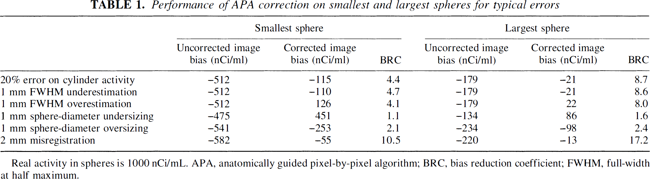
Real activity in spheres is 1000 nCi/mL. APA, anatomically guided pixel-by-pixel algorithm; BRC, bias reduction coefficient; FWHM, full-width at half maximum.

Figure 10 compares the relation between the SD and the bias for each sphere when there are some processing errors. These curves show that there is no direct relation between SD and bias. Even if SD always increases with bias, its evolution rate also depends on the origin of the error and on the sphere diameter. The corrected image SD is extremely sensitive to the presence of registration errors.

FIG. 10.

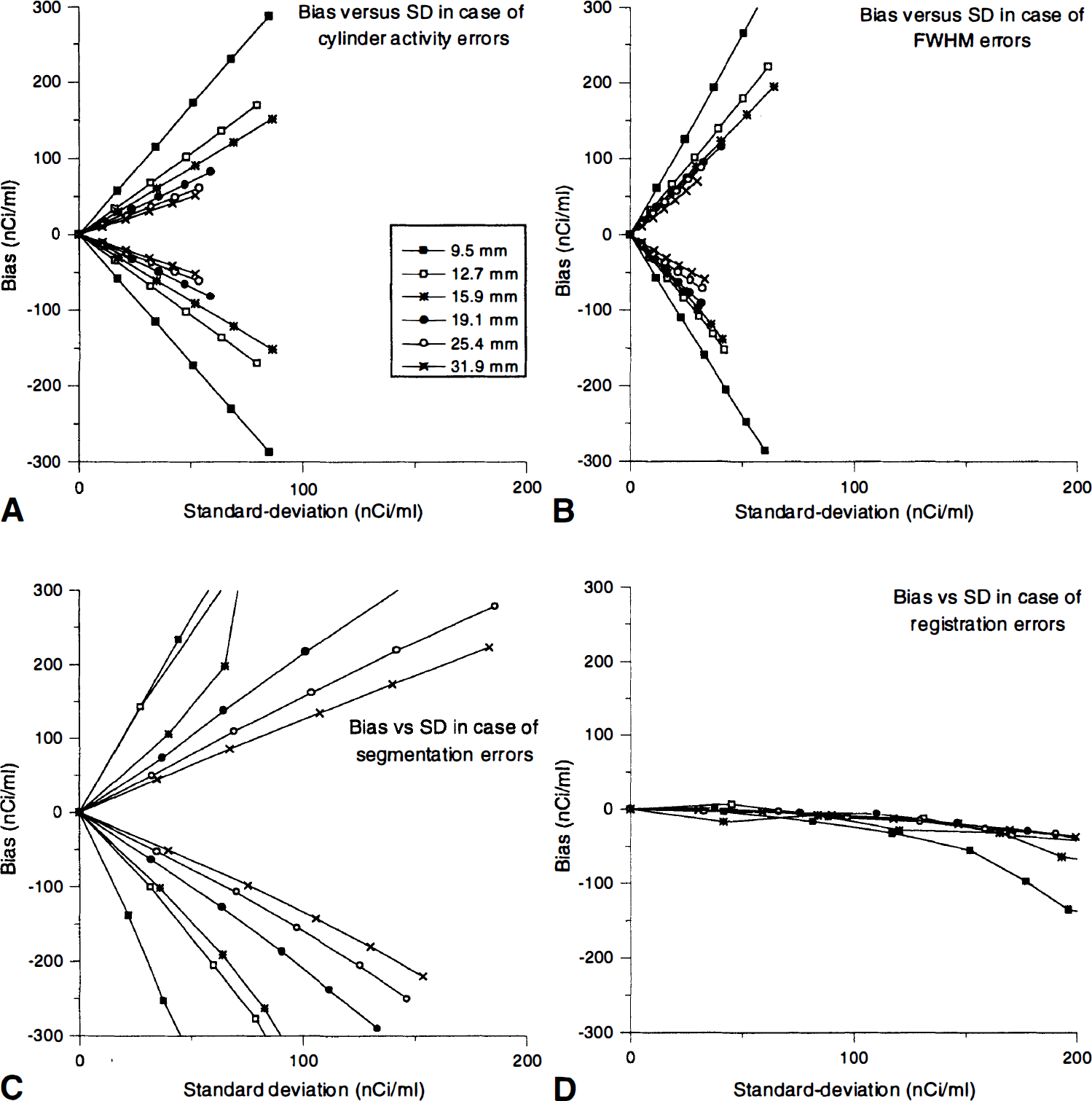
Relationship between SD and bias for each sphere in presence of parameter errors. (A) WM activity estimation. (B) Correction FWHM. (C) Segmentation errors (errors on sphere radiuses). (D) MRI-PET registration.

DISCUSSION

Previous studies suggest the strong influence of potential errors on the performance of APA correction. Videen and coworkers demonstrated the influence of misregistration errors on the binary correction for atrophy of PET simulations of a brain phantom (Videen et al., 1988). A later study of Meltzer and associates investigated the effects of misregistration and of incorrect segmentation thresholding on the binary correction of the brain PET image of a patient with Alzheimer's disease (Meltzer et al., 1990). The binary correction also was applied to a 16-cm sphere phantom, and the corrected image recovery coefficient was 79%, which is smaller than what was expected. An exhaustive error analysis was performed for the GM-PET method on computer PET simulations of a patient brain (Müller-Gärtner et al., 1992). Recently, the importance of this topic was underlined by Fahey et al., who presented a study on the accuracy of GM-PET (Fahey et al., 1996). All of these previous analyses were applied on complex brain images in which corrected structures are irregularly shaped and affected by interstructure spillover. On such images, it was difficult to conclude the effect of each correction step separately. The current work provides a comprehensive analysis of these issues by using simplified models, where all correction parameter and artefacts are more readily controlled and isolated.

The one-dimensional theoretical and experimental study demonstrated that each correction artefact exhibits a different and specific shape pattern, at least when the TT is larger than the system FWHM. Correction errors thus may be identified from visual examination. For instance, the presence of a spike on one structure edge and of a fall on the opposite edge is likely to indicate a registration error. Correct registration thus may be achieved by moving slightly the tissue images toward the spike. Once edge homogeneity is restored, a hypoactive or hyperactive structure outline would indicate either a segmentation error or an erroneous NT activity estimation (since these two errors produce artefacts that are more difficult to discriminate). The FWHM errors are less critical than the other errors, since this parameter can be optimized based on phantom studies before applying APA correction to real data. Notice that these conclusions were derived from one-dimensional examples where chosen structures were regularly shaped and at least bigger than 1 FWHM. However, they were observed for more complex structures in the current use of the GM-PET algorithm in our laboratory.

Correction artefacts are mainly located on the boundaries of the active structures, and this suggests that the robustness of the corrected measure may be improved by lessening or suppressing the influence of the edge voxels in the determination of the final measure. Several approaches may be used for this purpose: limiting the measurement region of interest (ROI) to small areas around the structure centers, or using suitable measurement statistics (Videen et al., 1988). However, remember that for small structures, edge artefacts propagate through the structure center. In that latter case, the approaches proposed earlier are insufficient to ensure accurate quantification.

The aim of the sphere phantom experiment was to determine which parameters were most determinant to ensure correction robustness. It appears unequivocal that the quality of tissue segmentation is critical in that matter. For small structures, segmentation errors may lead to dramatic biases, especially if active tissue dimensions are underestimated. Second comes the estimation of the NT activity and of the FWHM. Notice that the influence of the NT is likely to be even bigger when the TT is irregularly shaped. Finally, only severe registration errors (≈5 mm) may lead to significant biases, since the misregistration-induced artefacts have opposite directions and thus partly compensate for each other. However, this compensation effect requires that the measurement ROI covers both opposite artefacts; registration errors thus dramatically increase the influence of the ROI design strategy.

Another objective of the sphere phantom experiment was to determine a performance index to verify and quantify correction performance. Our initial estimation was that the regional SD could serve this purpose. The rationale for this choice was that SD strongly depends on ROI homogeneity, which is severely reduced by correction edge artefacts. As Figure 10 shows, SD is extremely sensitive to registration errors, and an increase in SD could appear even without any noticeable bias. Obviously, the design of reliable correction evaluation indexes requires taking into account the characteristic shapes of the correction artefacts. This could be achieved by independently computing statistics for the innermost and the outermost voxels. Segmentation or NT activity estimation errors then would be detected by comparing the center mean value and the boundary means value. Similarly, segmentation failure areas could be revealed by detecting local activity peaks.

In summary, APA correction provides a powerful tool for improving PET quantification, but its application to real data is limited by its lack of robustness. Precise segmentation and NT activity estimation are the most crucial issues to ensure a stable correction. The correction-induced artefacts arising from registration or segmentation inaccuracies exhibit characteristic shapes when the structures are big enough, which allows direct recognition from visual examination. Automated detection and removal of these artefacts, however, are more complex. The regional SD was assessed as a correction performance index, and our analyses show that it is inadequate as a global performance criterion, since it is overly sensitive to registration errors. The design of reliable performance indexes will require more sophisticated methods that should take into account the characteristic shape of each correction artefact.

Footnotes

Abbreviations used

APPENDIX

Consider the one-dimensional model presented on Fig. 1A. Since all of the tissues have similar bar shapes, the PSF blurring of their tissue distribution functions may be written as follows:

where the functions P₁ … ₄ are primitives of the PSF, centered on the locations x₁ & ₄:

By introducing these expressions into APA equation (3), we obtain the correction equation specific to our model:

The derivatives of C_TT(x) relative to the NT activity estimations are then

For the other parameters, we introduce the following notations:

Then, the partial derivatives of C_TT(x) relative to any parameter p except the NT activity estimations have the following form:

where the partial derivatives of P₁ & ₄ relative to x₀ and σ are, respectively,

Segmentation errors are assumed to affect only the TT, so that

These equations may be simplified in several manners, depending on the specific application. Notice in particular that, when a location x_i is distant enough (more than a few FWHM), its influence may be neglected by setting x_i ≈ –∞ (so that P_i(x) ≈ + 1/2) or x_i ≈ +∞ (so that P_i(x) ≈ −1/2). Also notice the binary correction, where no NT is acknowledged, so that equation (15) simplifies to

The derivatives of C_TT(x) then are readily computed as follows: (22)

\frac{\partial C_{T T}}{\partial p} (x) = - \frac{I_{o b s}}{(P_{1} - P_{2})^{2}} (\frac{\partial P_{1}}{\partial p} - \frac{\partial P_{2}}{\partial p}) (x)

Acknowledgments

The authors thank Vincent Brulon and Pascal Merceron for technical support, and Ken Moya for carefully reviewing the manuscript.

References

Bendriem

Dewey

Schlyer

Wolf

Volkow

(1991) Quantitation of the human basal ganglia with positron emission tomography: a phantom study of the effect of contrast and axial positioning. IEEE Trans Med Imaging 10:216–222

Chan

Herman

Levitan

(1997) A Bayesian approach to PET reconstruction using image-modeling Gibbs priors: implementation and comparison. IEEE Trans Nucl Sci 44:1347–1354

Di Chiro

Brooks

(1988) PET quantitation: blessing and curse [editorial]. J Nucl Med 29:1603–1604

Fahey

Gage

Harkness

(1996) Accuracy of the Mueller-Gaertner partial volume correction in brain PET. J Nucl Med 37:225P

Haber

Derenzo

Uber

(1990) Application of mathematical removal of positron range blurring in positron emission tomography. IEEE Trans Nucl Sci 37:1293–1299

Hoffman

Huang

Phelps

(1979) Quantitation in positron emission computed tomography. I. Effect of object size. J Comput Assist Tomogr 3:299–308

Kessler

Ellis

Jr Eden

(1984) Analysis of emission tomographic scan data: limitations imposed by resolution and background. J Comput Assist Tomogr 8:514–522

Knorr

Schüller

Scheitz

(1997) MRI based compensation of partial volume effect in PET image volumes. Neuroimage 5:S532

Kosugi

Sase

Suganami

Momose

Nishikawa

(1996) Dissolution of partial volume effect in PET by an inversion technique with the MR-embedded neural network model. In: Quantification of Brain Function Using PET ( Myers

Cunningham

Bailey

Jones

, eds), San Diego, Academic Press, pp 166–169

10.

Kuwert

Sures

Herzog

Jansen

Langen

K-J

Loken

(1993) The influence of image resolution on the positron emission tomographic measurement of caudate glucose consumption. Eur J Nucl Med 20:753–758

11.

Labbé

Froment

Kennedy

Ashburner

Cinotti

(1996) Positron emission tomography metabolic data corrected for cortical atrophy using magnetic resonance imaging. Alzheimer Dis Assoc Disorders 10:141–170

12.

Links

Leal

Mueller-Gaertner

Wagner

Jr (1992) Improved positron emission tomography quantification by Fourier-based restoration filtering. Eur J Nucl Med 19:925–932

13.

Mazziotta

Phelps

Plummer

Kuhl

(1981) Quantitation in positron emission computed tomography. V. Physical-anatomical effects. J Comput Assist Tomogr 5:734–743

14.

Meltzer

Kinahan

Greer

Nichols

Price

(1997) Evaluation of MR imaging-based partial volume correction methods for PET imaging. Radiology 205P:439

15.

Meltzer

Leal

Mayberg

Wagner

Jr Frost

(1990) Correction of PET data for partial volume effects in human cerebral cortex by MR imaging. J Comput Assist Tomogr 14:561–570

16.

Meltzer

Zubieta

Links

Brakeman

Stumpf

Frost

(1996) MR-based correction of brain PET measurements for heterogeneous gray matter radioactivity distribution. J Cereb Blood Flow Metab 16:650–658

17.

Müller-Gärtner

Links

Prince

Bryan

McVeigh

Leal

(1992) Measurement of radiotracer concentration in brain gray matter using positron emission tomography: MRI-based correction for partial volume effects. J Cereb Blood Flow Metab 12:571–583

18.

Natterer

(1988) Regularization techniques in medical imaging. In: Mathematics and Computer Science in Medical Imaging ( Viergever

Todd-Pokropek

, eds), Berlin, Springer-Verlag, pp 127–141

19.

Strother

Liow

J-S

Moeller

Sidtis

Dhawan

Rottenberg

(1991) Absolute quantitation in neurological PET. Do we need it? J Cereb Blood Flow Metab 11:A3–A16

20.

Strul

Bendriem

(1996) A phantom study of a MRI-based correction for partial volume effects in positron emission tomography. J Nucl Med 37: 154P

21.

Videen

Perlmutter

Mintun

Raichle

(1988) Regional correction of positron emission tomography data for the effects of cerebral atrophy. J Cereb Blood Flow Metab 8:662–670

22.

Yang

Huang

Mega

Lin

Toga

Small

(1996) Investigation of partial volume correction methods for brain FDG PET studies. IEEE Trans Nucl Sci 43:3322–3327.

Robustness of Anatomically Guided Pixel-by-Pixel Algorithms for Partial Volume Effect Correction in Positron Emission Tomography

Abstract

Keywords

THEORY

The anatomically guided pixel-by-pixel algorithm correction formulas

Factors of correction instability

Quality criteria

MATERIALS AND METHODS

Monodimensional bar experiment

Implementation of anatomically guided pixel-by-pixel algorithm correction

Simulation library

Quantitative analysis

Digital sphere phantom experiment

RESULTS

Monodimensional experiment

Digital sphere phantom

DISCUSSION

Footnotes

Abbreviations used

APPENDIX

Acknowledgments

References