Sage Journals: Discover world-class research

Abstract

A frequently reported limitation to using water as a tracer for measuring CBF has been the dependence of the CBF estimate on the experimental time (referred to as the failing flow phenomenon, FFP), To eliminate the FFP, we have developed the adiabatic solution of the tissue homogeneity model to replace the solution of the single-compartment Kety model. In Part I, the derivation of the adiabatic solution was presented, In this second part, the adiabatic solution was applied to measure CBF in rabbits using nuclear magnetic resonance spectroscopy and the tracer deuterium oxide, It was shown that the FFP, observable when the ²H clearance data were analyzed with the Kety equation, was significantly reduced when the same data were analyzed with the adiabatic solution of the tissue homogeneity model. By concurrently measuring CBF with radioactive microspheres, it was determined that the CBF estimates from the adiabatic solution were accurate for true blood flow values less than 60 mL·100 g⁻¹·min⁻¹, Above this value the CBF estimate was progressively underestimated, which was attributed to the diffusion limitation of water in the brain.

Keywords

Cerebral blood flow Tracer kinetics Deuterium oxide Nuclear magnetic resonance spectroscopy

In Part I, it was demonstrated that a time-domain, closed-form solution to the tissue homogeneity (TH) model (Johnson and Wilson, 1966; Sawada et al., 1989) can be derived using the adiabatic approximation, The motivation for this work was to develop a model that, on the one hand, is realistic enough to overcome the limitations of the Kety model in describing water transport in the brain (Kety, 1951), while, on the other hand, being simple enough to be useful in the analysis of data with limited temporal resolution.

The derived solution, or the adiabatic solution, was used to analyze ²H-labeled water (D₂O) clearance data from the brain that was acquired using nuclear magnetic resonance spectroscopy, This technique was chosen because it provided data with good signal-to-noise ratio, Since D₂O was injected into a peripheral vein and the arterial blood concentration of the tracer was determined throughout the experiment, the experimental procedure was analogous to that used in human studies with positron emission tomography (PET) (St. Lawrence et al., 1992), Additional steps were taken to ensure that other possible sources of the falling flow phenomenon (FFP) were accounted for in the experimental protocol. Such sources include timing errors in the input function (Iida et al., 1986, Koeppe et al., 1987), dispersion of the true input function (Iida et al., 1986), tissue heterogeneity (Gambhir et al., 1987), and arterial blood contamination (Koeppe et al., 1987, Ohta et al., 1996). Finally, the CBF estimates derived from the adiabatic solution were verified by concurrent measurements with radioactive microspheres (Heymann et al., 1977).

THEORY

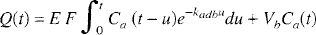
The theoretical modeling that formed the basis for the data analysis in this study was outlined in Part I. The ²H clearance data were analyzed with both the Kety equation (Equation 1 in Part I) and the adiabatic solution to the TH model (Equation 14 in Part I), As discussed in Part I, for either solution CBF was determined from the exponential rate constant, which characterized the clearance of labeled water from brain tissue. For reference, the rate constant for the Kety equation is

k_{1 c} = \frac{E F}{λ},

(1)

where λ is the partition coefficient, E is the extraction fraction of water, and F is the blood flow of the tissue. For the adiabatic solution to the TH model, the rate constant is

k_{a d b} = \frac{E F}{V_{e}}

(2)

where V_e is the volume of water in the extravascular space (EVS) of the tissue.

Effect of the arterial signal

The modeling process outlined in Part I only describes tracer transport in the microvasculature. Under experimental conditions, it is likely that larger vessels will contribute to the signal from the tissue (Feindel et al., 1965; Koeppe et al., 1987; Ohta et al., 1996). This additional vascular signal can be accounted for in the adiabatic solution (Equation 14 in Part I) by replacing the parameter V_i, which is the distribution volume of water in the microvasculature (IVS), with a larger vascular volume, V_b, that represents the volume of all blood-borne signal, including V_i

Q (t) = E F \int_{0}^{t} C_{a} (t - u) e^{- k_{a d b} u} d u + V_{b} C_{a} (t)

(3)

Effect of internal dispersion

It has been shown that the shape of the arterial blood curve measured at a peripheral artery can be distorted compared with the shape of the curve in the brain (Iida et al., 1986). This distortion is caused by the difference in the dispersion of the tracer as it passes from the heart to the brain compared with the dispersion from the heart to the peripheral arterial sampling site. Internal dispersion can be characterized by the following function (Iida et al., 1986)

d_{i} (t) = \frac{1}{τ} \exp (\frac{- t}{τ})

(4)

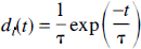
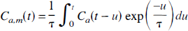
where di(t) is the internal dispersion function and τ is the internal dispersion time constant. The measured arterial blood curve, C_a,m(t), at the peripheral site is related to the true arterial function, C_a(t) by

C_{a, m} (t) = \frac{1}{τ} \int_{0}^{t} C_{a} (t - u) \exp (\frac{- u}{τ}) d u

(5)

Using Equation 5, the Kety equation (Equation 1 in Part I) can be expressed in terms of the measured arterial blood curve

Q (t) = F τ C_{a, m} (t) + F (1 - τ k) \int_{0}^{t} C_{a, m} (t) e^{- k_{1 C} (t - u)} d u

(6)

Equation 6 has a form similar to the adiabatic solution (Equation 3). That is, the effects of internal dispersion and diffusion limitation of the tracer both lead to a fraction of the arterial blood curve being required in the solution for Q(t). Therefore, the effect of internal dispersion must be determined separately if the diffusion limitation of water is to be investigated independently. A simple “bench top” experiment, which is outlined in the next section, was carried out to determine the effect of internal dispersion.

METHODS

Experimental procedure

Cerebral blood flow was measured in male New Zealand rabbits weighing 2.5 to 3.0 kg. Before an experiment, the rabbit was administered a preoperative dose of ketamine and xylazine (35 mg/kg ketamine mixed with 5 mg/kg xylazine) by intramuscular injection. An ear vein was catheterized and a tracheotomy performed while the rabbit was masked with 5% halothane. The rabbit was then ventilated with a mixture of O₂ and 1.5% isoflurane and paralyzed with an intravenous injection of pancuronium bromide (0.3 mg/kg), which was repeated at 1-hour intervals throughout the experiment. Catheters were inserted into a femoral vein, an ear vein, both femoral arteries, and the left atrium of the heart. To avoid signal contamination from scalp tissue, it was retracted to allow the surface coil to be placed directly on the skull.

After surgical preparation, the rabbit was wrapped in a re-circulating water heating pad to maintain rectal temperature at 37°C. A three-turn surface coil with a diameter of 1.6 cm was placed on the rabbit's skull, and the rabbit together with the surface coil were positioned in the center of a horizontal bore Oxford magnet with a field strength of 1.89 T. Data acquisition was controlled by a Multi-Spec-IV2 console from Surrey Medical Imaging Systems (Surrey, U.K.). Arterial blood pressure was monitored throughout the experiment by means of a transducer connected to a femoral arterial catheter, and if required, phenylephrine (0.2 mg/mL) was infused into the ear vein to ensure that mean arterial blood pressure was maintained within the normal range (75 to 100 mm Hg). Before each CBF measurement, the blood gases were repeatedly measured to ensure they remained stable over a period of at least a half hour. Cerebral blood flow was measured twice in each animal, and the P_aco₂ was varied between trials (from 25 to 60 mm Hg) to obtain a range of CBF values. After each trial, the blood gases were again measured to determine whether the levels had remained constant during the experiment.

After the stabilization period, 10 mL of 99.1% D₂O with 0.9% NaCl was infused for 30 seconds into the femoral vein catheter. In none of the rabbits did the D₂O infusion cause any changes in the arterial blood pressure. An adiabatic radio frequency pulse, having its amplitude modulated by a hyperbolic secant function, was used for uniform excitation of the ²H nuclei in the brain (Baum et al., 1985). The repetition time between successive pulses was 750 ms, which was chosen to allow the ²H nuclei sufficient time to return to equilibrium before the next radio frequency pulse. The ²H signal, which was the average of four free-induction decays (FID), was collected every 3 seconds. Owing to the rapid hydrogen—deuterium exchange, this signal reflected singly deuterated water HOD concentration in the brain (Ackerman et al., 1987). The ²H data were collected for 1 to 2 minutes before injection (background signal) and for 15 minutes after injection. To determine the ²H concentration in arterial blood during the experiment, arterial blood samples were collected at known time intervals throughout the experiment. The blood was withdrawn at a rate of 0.3 mL/min by a peristaltic pump connected to a femoral artery catheter. Using a fraction collector, the blood samples were collected over the following time intervals: 6 seconds for the first 3.5 minutes, 12 seconds for the next 3 minutes, and 30 seconds for the last 8.5 minutes. The concentration of HOD in each sample was determined after the experiment using the procedure described below.

Immediately after the completion of a D₂O washout experiment, CBF was measured using radioactive microspheres (Heymann et al., 1977). For the microspheres experiment, arterial blood was drawn from a femoral catheter at a rate of 1 mL/min for 3 minutes. At the 1-minute mark, 10 µCi of radioactive microspheres were injected into the left atrium. After the completion of both ²H clearance trials and their respective microspheres experiments, the rabbit was killed and the brain removed. The brain was cut into small samples and each sample weighed. The content of radioactive microspheres in the tissue samples and the blood reference samples were assayed, and from this data, CBF was determined for each brain sample (Heymann et al., 1977).

The relative concentration of HOD in each of the blood samples collected during a D₂O washout experiment was determined using a small solenoid coil placed in the 1.89 T magnet (St. Lawrence et al., 1992). The number of FID collected for each sample depended on the time interval in which the sample was collected: 512, 200, and 64, respectively, for the time intervals listed previously. The measurement (see next paragraph) from each blood sample was scaled according to its weight and the number of FID averaged.

For both the tissue and the arterial blood data, processing consisted of multiplying each averaged FID with an exponential filter (4-Hz line-broadening factor), finding the complex frequency spectrum by fast Fourier transform, and calculating the magnitude of the complex frequency spectrum afterward. Each magnitude spectrum was then integrated with respect to frequency to determine the area under the ²H peak. The individual peak areas were corrected for the background signal by subtracting the average peak area value determined from spectra collected before the injection of the D₂O. There were between 20 and 40 background spectra collected for the tissue data, and 5 for the arterial blood data.

Signal detection

As mentioned previously, the ²H signal from the brain was detected using a surface coil. The finite extent and nonuniformity of the surface coil's field of reception of radio frequency waves necessitated the following modifications to Equation 3. To begin with, because the boundaries of the coil's sensitivity volume were not well defined, it was assumed that the coil detected signal originating from both gray and white matter in the brain (Ewing et al., 1989). To account for the signal from these two types of tissue, the adiabatic solution was summed over two rate constants in which the faster one represented blood flow in gray matter and the slower one represented blood flow in white matter (Obrist et al., 1967). In addition, the coil's sensitivity to gray and white matter would be different depending on their respective locations relative to the coil. To account for these factors, Equation 3 was modified as

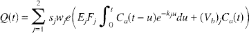
Q (t) = \sum_{j = 1}^{2} s_{j} w_{j} e (E_{j} F_{j} \int_{0}^{t} C_{a} (t - u) e^{- k_{j} u} d u + (V_{b})_{j} C_{a} (t))

(7)

where the subscript j referred to either gray or white matter. All variables were defined previously, except w_j, which was the relative weight (fraction) of the jth type of tissue, and s_j, which represented the sensitivity of the coil to this tissue type. It was impossible to determine s_j without knowing the exact location of the jth tissue type relative to the coil. Consequently, although an individual CBF for each of the two tissue types could be determined from their respective rate constants, without knowing the s_j, the mean CBF for the specific mixture of gray and white matter in the sensitivity volume of the coil could not be determined.

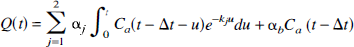
Data analysis

In the curve-fitting analysis, all parameters before the integral sign for each tissue type in Equation 7 were lumped together as a single fitting parameter α_j, and the vascular volumes were combined as a single term a_bC_a(t). It is important to note that the fitting parameter, α_j, could not be used as a measure of the relative weight of the jth tissue since this parameter was also dependent on s_j. Because of the nonuniformity of the spatial sensitivity of the surface coil, s_j could not be determined, and therefore, its effect on the magnitude of α_j was unknown. A time shift (Δt) between the two data sets (the tissue and arterial blood concentration of HOD was included in the fitting routine to account for the difference in time between the arrival of the tracer in the brain and the arrival of the tracer at the fraction collector (Meyer, 1989)

Q (t) = \sum_{j = 1}^{2} α_{j} \int_{0}^{t} C_{a} (t - Δ t - u) e^{- k_{j} u} d u + α_{b} C_{a} (t - Δ t)

(8)

A constrained quasi-Newton algorithm was used in the regression analysis (Gill and Murray, 1974) to estimate the parameters in Equation 8. Besides the adiabatic solution of the TH model, the Kety equation was also used in the analysis. The Kety equation was also summed over two tissue types and its operational equation was given by Equation 8 without the a_bC_a(t) term. Note that in Equation 8 the subscript lc or adb on the rate constant was omitted. This omission was deliberate as the definition of a rate constant was not relevant to the regression analysis. When CBF was determined from the estimated rate constant, it was necessary to use either Equation 1 or 2, depending on the solution used in the analysis. For both solutions, the rate constants and scaling factors were constrained to have positive values since any negative values were nonphysiologic. A piecewise cubic Hermite interpolation routine was used to interpolate the arterial data to the same sampling interval as the tissue data (Gill and Murray, 1974).

To determine whether the estimates of the rate constants were independent of the experimental duration, the regression analysis was repeated using the Kety equation and the adiabatic solution with an increasing amount of data included with each successive repetition. The analysis began with the first 4 minutes of clearance data (the time of the initial rise of the ²H clearance curve above background was taken as zero time), and with each repetition, an additional 1 minute of data was included in the analysis until the end of the clearance data set was reached (15 minutes). A starting duration of 4 minutes was chosen because the clearance data did not reach its maximum value until roughly 2.5 minutes after injection because of the relatively long infusion duration (30 seconds) and the convolution of the data with the dispersion function of the sampling apparatus (see next section). For each increment, the percent difference of the higher rate constant (k₁) determined for the entire experimental duration from that determined for that time duration was calculated. The results were divided into two categories: (1) k₁ values corresponding to CBF measurements obtained using radioactive microspheres (CBF_M) that were less than 60 mL·100 g⁻¹·min⁻¹ (referred to as the flow-limited category), and (2) k₁ values corresponding to CBF_M values that were greater than 60 mL·100 g⁻¹·min⁻¹ (referred to as the diffusion-limited category). The value of 60 mL·100 g⁻¹·min⁻¹ was chosen as the boundary between these two categories because E was approximately 0.9 at this flow value (assuming PS = 150 mL·100 g⁻¹·min⁻¹; Herscovitch and Raichle, 1987), and therefore, above this flow value, the effect of the diffusion limitation of water on the CBF estimate should become noticeable. With regard to the Kety equation, if the diffusion limitation of water were the primary factor contributing to the FFP, then the FFP should have been negligible for the flow-limited group since E was close to one. On the other hand, if there were a significant contribution from the larger vessels, then the FFP should have been observable at all flow values since this factor was independent of the diffusion limitations of the tracer (Koeppe et al., 1987). For the adiabatic solution, the FFP should not be present in either category since the α_bC_a(t) term in Equation 8 had already accounted for all of the vascular signal. This analysis was not repeated for the lower rate constant (k₂) because of its significantly lower precision as compared with the precision of k₁ (see Fig. 6 in Part I).

External dispersion

A 1.0-m length of PE 60 surgical tubing (1.1 mL volume) was used to connect the fraction collector to the arterial catheter. This length of tubing was required to keep the sampling apparatus at a sufficient distance away from the magnet so as not to affect the detection of the ²H signal. The presence of the tubing led to two artifacts in the measured arterial curve: a time delay with respect to the tissue data and a dispersion with respect to the true arterial curve. The time delay was accounted for in the regression analysis by the time shift variable discussed previously. The dispersion artifact was characterized by performing the following experiment.

The arterial blood sampling tubing, together with the arterial catheter and a three-way stopcock, was filled with saline. At time zero, one end of the tubing was dipped into a mixture of blood and D₂ O. Using the peristaltic pump, samples were collected at 6-second intervals for 4 minutes after the submersion of one end of the tubing in the mixture, and the procedure was repeated four times. The HOD concentration in each sample was measured using the same procedure as with blood samples from the CBF experiments. The dispersion of a known input function can be expressed mathematically as (Iida et al., 1986)

C_{m} (t) = \int_{0}^{t} C_{t r u e} (t - u) d i s p (u) d u

(9)

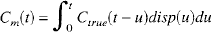
where C_true(t) is the known input function, C_m(t) is the measured function, and disp(t) is the dispersion function. In the dispersion experiments, the input function was a step function, which reduced Equation 9 to

C_{m} (t) = \int_{0}^{t} d i s p (u) d u

(10)

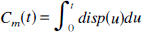
The dispersion function, disp(t), was assumed to be the sum of two gamma variate functions. The parameters of the gamma variate functions were determined by fitting Equation 10 to the measured curve, C_m(t), using nonlinear regression techniques (Gill and Murray, 1974).

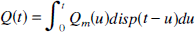
In principle, knowing the dispersion function of the sampling system, the true arterial blood curve could be determined by deconvolution. Instead, for the CBF experiments, the tissue data were convolved with disp(t), which was equivalent to deconvolving the arterial data but easier to implement. If Q_m(t) was the measured tissue curve, then the dispersed tissue curve, which was the data to be fitted by Equation 8 using nonlinear regression analysis, was given by

Q (t) = \int_{0}^{t} Q_{m} (u) d i s p (t - u) d u

(11)

Internal dispersion

For these experiments, iodinated x-ray contrast agent (Isovue 300) was used as a tracer so that its concentration could be measured using the principle of absorptiometry (Yeung and Lee, 1992). The experimental setup consisted of a length of tubing with an internal diameter of 0.28 cm, a peristaltic pump, and the absorptiometry unit (Yeung and Lee, 1992). One end of the tubing was passed through the peristaltic pump before it was connected to the absorptiometry unit. The tubing had an additional 90-cm removable section that represents the distance from the left ventricle to the radial arteries in humans. This section was removed in baseline experiments and attached in the experiments designed to simulate dispersion in arteries. Before each experiment, the tubing was filled with water and, at time zero, the free end of the tubing was dipped into a reservoir of contrast solution (20 mg iodine/mL). The solution was pumped through the tubing at a rate (7 to 18 cm/s) controlled by the peristaltic pump, and the dispersion of the contrast agent was measured by the absorptiometry unit. Using the assumed internal dispersion function for arteries (Equation 4), the measured baseline dispersion curve was deconvolved with the measured arterial dispersion curve to determine the internal dispersion time constant τ.

RESULTS

Data analysis

A total of 44 trials (2 per rabbit) were attempted on 22 rabbits, with blood flows ranging from 30 to 150 mL·100 g⁻¹·min⁻¹. Six of the trials failed because of either technical errors or a change in Paco₂ greater than 3 mm Hg in the rabbit during the experiment. The data obtained from one experiment are illustrated in Fig. 1. In the figure, time zero had been arbitrarily set to correspond to the time of the initial rise of the ²H clearance curve above background, and the data before time zero represented the background values. The arterial data set had been shifted to the right to account for the time delay introduced by the arterial blood sampling apparatus. In the subsequent regression analysis, the relative positions of these two sets of data on the time axis were not important because a time shift (Δt) variable had been included as a fitting parameter. The data were presented in relative units only because no calibration between the blood and tissue data was performed owing to the nonuniform spatial sensitivity of the surface coil. However, calibration was not necessary because CBF were determined from the rate constants only.

FIG. 1.

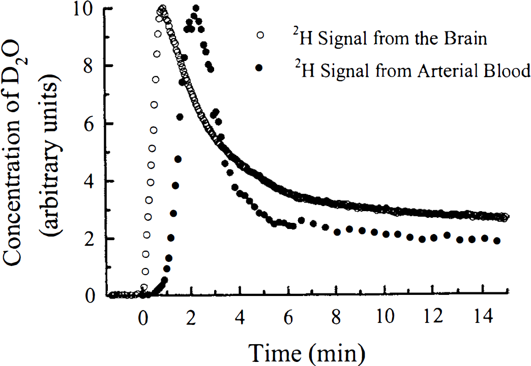
The brain and arterial blood concentration of HOD as measured by nuclear magnetic resonance spectroscopy in a rabbit experiment. The brain and the arterial blood concentrations, both in arbitrary units, were plotted as functions of time. The time of the initial rise of the tissue data above background noise after the infusion of the D₂O was assumed to be time zero.

For both the Kety equation and the adiabatic solution, the time dependency of k₁ is illustrated in Fig. 2 for the 36 successful trials. The mean percent difference in k₁, as a function of experimental duration was plotted for the flow-limited group and the diffusion-limited group. From this graph it was apparent that the FFP was quite dramatic for both flow groups when the data were analyzed using the Kety equation. In comparison, the FPP was reduced considerably when the data were analyzed using the adiabatic solution of the TH model.

FIG. 2.

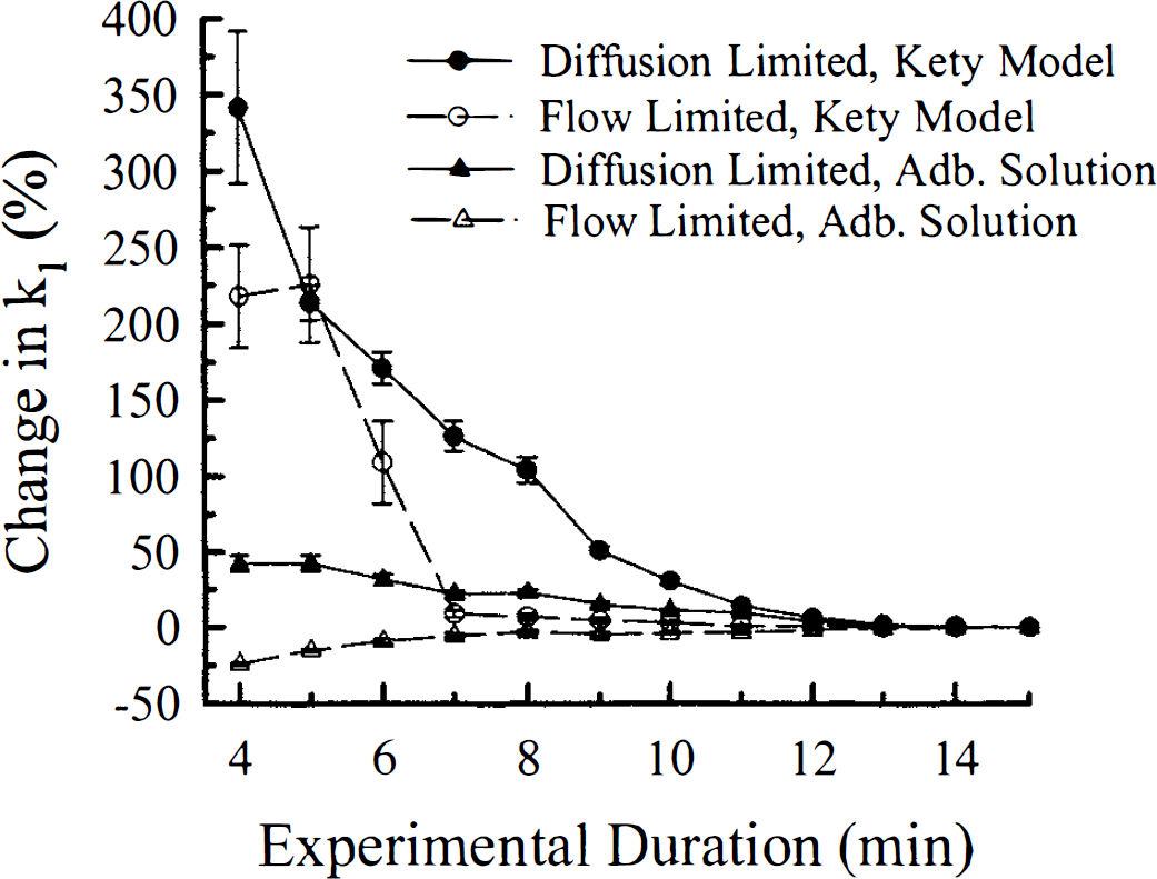
The plot of percent difference of k₁ determined for the entire experimental duration from that determined for a particular experimental duration versus experimental duration. The data were divided into two groups: (1) CBF less than 60 mL·100 g⁻¹·min⁻¹ (flow-limited group), and (2) CBF greater than 60 mL·100 g⁻¹·min⁻¹ (diffusion-limited group). There were 12 trials in the flow-limited group and 24 trials in the diffusion-limited group. All data were analyzed using both the adiabatic solution of the tissue homogeneity model and the Kety equation. The data plotted were the mean percent differences of k₁ for each group, estimated using both solutions. The error bars were the standard errors of each group at the specific experimental duration. Adb., adiabatic.

For validation, the estimate of gray matter blood flow (CBF_g) from k₁, as defined by Equation 2, was compared with the CBF_M for samples of tissue that were located just beneath the surface coil and were comprised mainly of cortical gray matter. Using a value of 94 mL·100 g⁻¹ for V_e (Herscovitch and Raichle, 1985), CBF_g was calculated for all 36 trials using the higher rate constant estimated from the entire experimental duration. The CBF_g values are plotted in Fig. 3 as a function of the corresponding CBF_M measurements. The estimated value of the PS product for water was 140 mL·100 g⁻¹·min⁻¹, which was obtained by fitting Equation 4 from Part I to the data (Crone, 1963). This value was in good agreement with previously reported values for the PS product of the cerebral cortex (Herscovitch and Raichle, 1987).

FIG. 3.

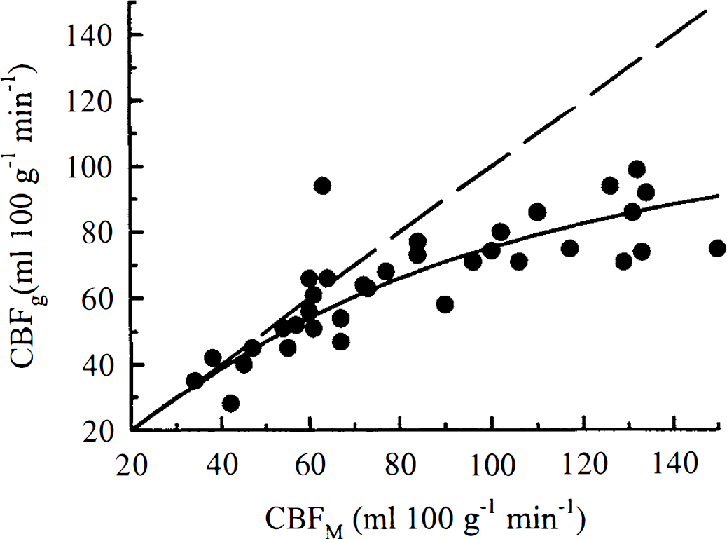
The correlation between cortical gray matter CBF estimated by the adiabatic solution (CBF_g) and by radioactive microspheres techniques (CBF_M). A total of 36 trials are presented and the dashed line is the line of identity. By fitting Equation 3 to the data, the PS product was estimated to be 140 mL·100 g⁻¹·min⁻¹.

Because of the mixing of gray and white matter in the other brain samples, an estimate of white matter blood flow was not obtained from the microspheres data. As a result, the CBF estimate from the lower rate constant, which represented white matter blood flow, could not be validated. Instead, the correlation between the k₂ estimates from the regression analysis and CBF_M is presented in Fig. 4. Although CBF_M represented gray matter blood flow, this graph did show the high degree of scatter in k₂, which was caused by the low precision associated with this parameter. In Part I, we estimated that the coefficient of variation (CV) of k₂ was approximately 22%, which was considerably higher than the CV of k₁ (≈7%). This reduction in precision can be attributed to the smaller weighting factor for this rate constant. Although the weighting factor for white matter is generally smaller than that of gray matter because of the lower blood flow in white matter, the value is further reduced by the surface coil's nonuniform sensitivity. The coil was most sensitive to the tissue immediately beneath it, which was cortical gray matter.

FIG. 4.

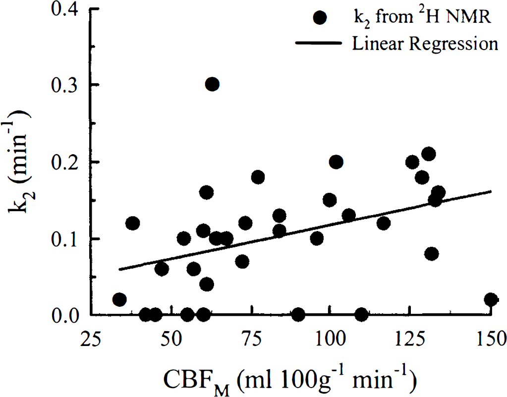
The correlation between k₂, as determined from the adiabatic solution, and CBF measured using radioactive microspheres (CBF_M). The results for the linear regression analysis were slope, 9 × 10⁻⁴; intercept, 0.03; and regression coefficient, 0.46; the relationship was statistically significant (P < 0.05).

External dispersion

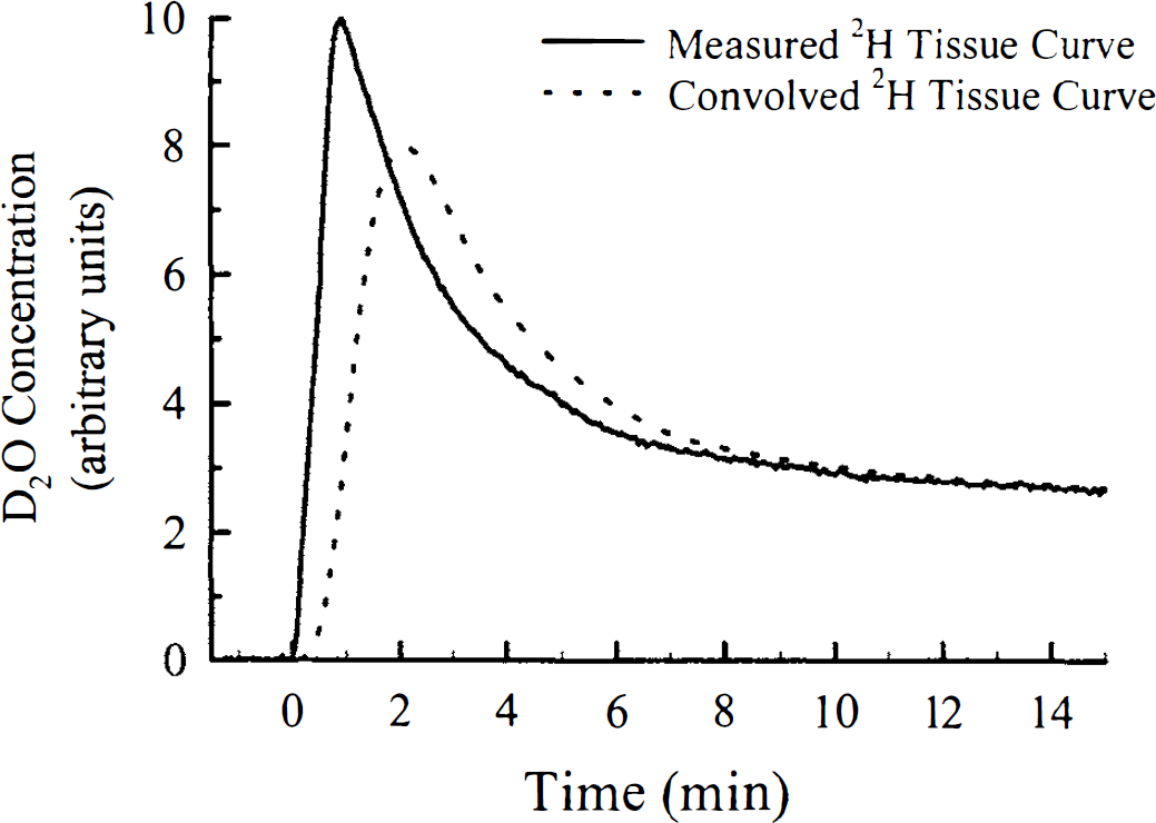
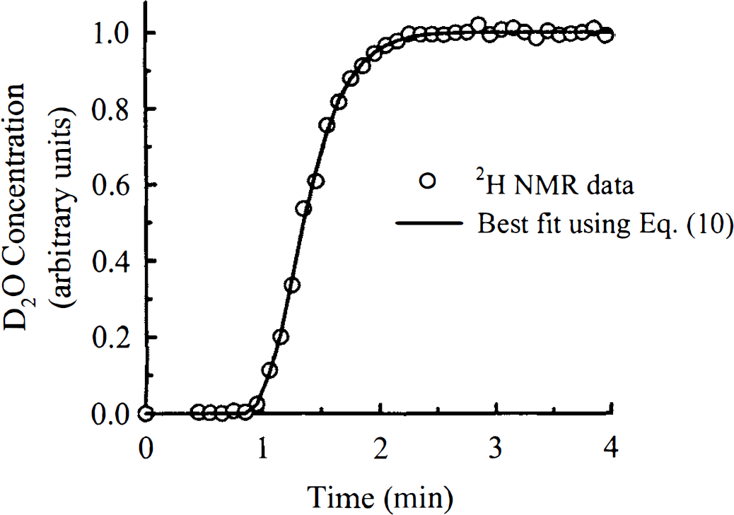
In Fig. 5, the averaged data set from the four trials of the external dispersion experiment is illustrated with the fit to the data using Equation 10 superimposed. The excellent agreement indicated that the dispersion caused by the blood sampling apparatus could be well represented by the sum of two gamma variate functions, which was the assumed external dispersion function. Figure 6 shows the convolution of the tissue curve from Fig. 1 with the external dispersion function in Fig. 5.

FIG. 5.

The fit to the measured step-function response from the external dispersion experiments using Equation 10 is superimposed on the experimentally data. The external dispersion function used in the regression analysis was the sum of two gamma variate functions. The data shown were collected with a 6-second sampling interval and represent the average of four experiments.

FIG. 6.

The result of the convolution of the measured tissue clearance curve, which is displayed in Fig. 1, with the dispersion function of the blood sampling apparatus. It was the convolved data set that was fitted with Equation 8 to determine CBF.

The CV of the residuals of the averaged data set displayed in Fig. 5 from the fitted dispersion function was 1.3%. Using the covariance matrix method, which was outlined in Part I, we determined that the CV for any of the parameters defining the external dispersion function (see Equations 9 –11) was less than or equal to 3%. By sequentially changing each parameter of the external dispersion function by two standard deviations, we determined that the largest expected error in the k₁ and k₂ estimates would be 3% and 7%, respectively. Therefore, any possible error in the characterization of the dispersion caused by the sampling apparatus would not significantly influence the CBF measurements.

Internal dispersion

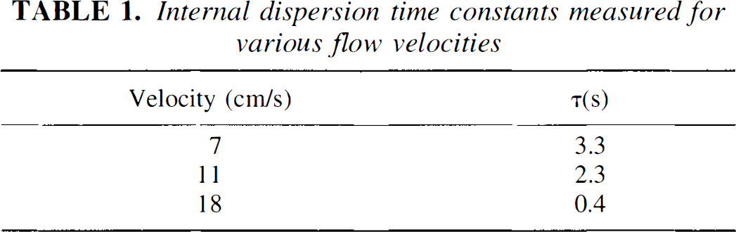
The internal dispersion time constants measured for various flow velocities in the internal dispersion experiments are given in Table 1. For comparison, using color flow Doppler ultrasound the mean blood flow velocity in the radial artery of one volunteer was measured to be 18 cm/s. Because the path length difference found in the rabbit experiments was significantly shorter than 90 cm, the dispersion time constant must have been less than 0.4 seconds. Therefore, the influence of internal dispersion on the shape of the arterial curve would be negligible.

DISCUSSION

As demonstrated by the results in Fig. 2, the FFP was observable in both the flow-limited group and the diffusion-limited group when the data were analyzed using the Kety equation. In the literature, various factors that may contribute to the FFP have been investigated. These factors included (1) tissue heterogeneity (Gambhir et al., 1987), (2) timing errors in the input function (Iida et al., 1986, Koeppe et al., 1987), (3) dispersion of the input function (Iida et al., 1986), (4) the inadequacy of the single-compartment model (Gambhir et al., 1987; Larson et al., 1987; Ohta et al., 1996), and (5) signal contamination from arterial blood (Koeppe et al., 1987; Ohta et al., 1996). Tissue heterogeneity could be disregarded as a possible explanation in this study because both the Kety equation and the adiabatic solution were summed over two tissue types. To avoid any error resulting from a time shift between the ²H signal in tissue and in arterial blood, a time shift variable was included as a fitting parameter in the regression analysis (Meyer, 1989). Dispersion of the input function (arterial curve) could occur within both the subject (internal dispersion) or the sampling apparatus (external dispersion). The results in Table 1 demonstrated that the internal dispersion time constant was small for the flow velocities found in arteries, which were typically greater than 18 cm/s. Considering that the path difference within a rabbit was much shorter than the 90-cm length of tubing used in the experiments of Table 1, internal dispersion must have been insignificant in the rabbit experiments. External dispersion, although present, was explicitly accounted for by determination of the external dispersion function in separate dispersion experiments outlined previously. Therefore, in our CBF experiments neither source of dispersion could be considered the cause of the FFP.

TABLE 1.

Internal dispersion time constants measured for various flow velocities

Velocity (cm/s)	τ(S)
7	3.3
11	2.3
18	0.4

We believe that the FFP arises from the remaining two factors: inadequacy of the Kety model in describing water transport in the brain and signal contamination from arterial blood. It has been demonstrated theoretically that water transport in the brain would be better described by a two-compartment model (Gambhir et al., 1987). Our data support this hypothesis and complement the findings of Ohta et al. (1996), who investigated the effect of a vascular contribution on CBF measurement using PET and the tracer H₂¹⁵O. As the results in Fig. 2 illustrated, when the Kety model was used to analyze data from the diffusion-limited group, there was a consistent decrease in the k₁ estimate as the experimental duration increased. By using the adiabatic solution instead of the Kety equation, the trend was significantly reduced, although not entirely eliminated. Even with the adiabatic solution, the mean k₁ for the 4 minutes of experimental time was 40% greater than k₁ for the entire experimental duration, which was attributed to the correlation between the fitting parameters α_b and k₁ (see Table 3, Part I). As discussed in the previous article, the correlation between these two parameters could be eliminated by increasing the experimental duration to more than 9 minutes. There was also a bias introduced into the k₁ estimate derived from the analysis with the Kety equation, which was the result of the constraints imposed in the regression analysis. However this bias was not large enough to explain the FFP associated with this model. Therefore, the observed FFP must be a result of the inadequacy of the Kety model in accounting for the diffusion limitation of labeled water.

If the FFP were only a result of the diffusion limitation of the tracer in the microvasculature, then it should not have been observed for the flow-limited group when the data were analyzed with the Kety equation. However, the results illustrated in Fig. 2 showed a large overestimation of k₁ for early integration times, although for times greater than 6.5 minutes the k₁ estimate was stable. We believe that this overestimation of k₁ was a result of the blood-borne signal arising from outside the capillary space, such as from a major artery. The significance of the arterial blood volume has been recently demonstrated by Ohta et al. (1996). Using PET they were able to generate maps of the vascular volume, and from these maps it was clearly demonstrated that the vascular volume increased dramatically near major arteries. With the adiabatic solution, the arterial blood-borne signal was accounted for by the term α_bC_a(t), and as a result, the estimate of k₁ was relatively stable over all integration times for the flow-limited group.

Even though the adiabatic solution significantly reduced the FFP, the results in Fig. 3 demonstrated that this solution was only able to accurately measure CBF at flow rates less than 60 mL·100 g⁻¹·min⁻¹. Above this threshold, the CBF estimate was appreciably underestimated because of the limited extraction of water into the parenchymal tissue. These results were similar to what had been previously reported for CBF measurements using the tracer H₂¹⁵O (Raichle et al., 1983). It had been demonstrated that if CBF was to be measured accurately at all values, then compartmental models had to be abandoned in favor of the more physiologically realistic distributed-parameter models (Goresky et al., 1976; Rose et al., 1977; Larson et al., 1987). Unfortunately, as discussed in Part I, the solutions to distributed-parameter models were considerably more complex than the adiabatic solution. Furthermore, there were other experimental limitations that had to be considered, such as (1) the arterial blood-borne signal, and (2) tissue heterogeneity. Regardless of the model chosen, these factors will influence the CBF estimate if they are not accounted for in the modeling. A distributed-parameter model had been used to analyze data acquired with PET, and it was concluded that owing to the noise limitations of PET images, implementing such a model was unrealistic (Quarles et al., 1993). For our study the adiabatic solution represented a reasonable compromise between experimental reality and the true complexity of water transport in the brain.

In summary, experimental data were presented that verified the ability of the adiabatic solution of the TH model to properly describe the transport of water in the brain. From the data analysis, it was determined that the adiabatic solution was capable of significantly reducing the FFP that was observed when clearance data were analyzed with the Kety equation. By accounting for other possible sources of the FFP, we believe this phenomenon can be attributed to the diffusion limitation of water and the arterial blood-borne signal. For validation of the adiabatic solution, CBF was concurrently measured with radioactive microspheres. By comparing the microspheres CBF estimates with the estimates from the adiabatic solution, it was also demonstrated that the latter could accurately measure CBF for flow values less than 60 mL·100 g⁻¹·min⁻¹. Above this value, the diffusion limitation of water resulted in a progressive underestimation of CBF by the adiabatic solution as the true value of CBF increased.

Footnotes

Acknowledgments

The authors thank Monique Labodi and Jane Sykes for their technical assistance. The authors also thank Sarah Henderson and Dr. Ivan Yeung for their many valuable suggestions.

Abbreviations used

References

Ackerman

JJH

Ewy

Becker

Shalwitz

(1987) Deuterium nuclear magnetic resonance measurements of blood flow and tissue perfusion employing ²H₂O as a freely diffusible tracer. Proc Natl Acad Sci USA 84:4099–4102

Baum

Tycho

Pines

(1985) Broadband and adiabatic inversion of a two-level system by phase-modulated pulses. Phys Rev 32: 3435–3447

Crone

(1963) The permeability of capillaries in various organs as determined by use of the ‘indicator diffusion’ method. Acta Physiol Scand 58:292–305

Ewing

Branch

Helpern

Smith

Butt

Welch

KMA

(1989) Cerebral blood flow measured by NMR indicator dilution in cats. Stroke 20:259–267

Feindel

Garretson

Yamamoto

Perot

Rumin

(1965) Blood flow patterns in the cerebral vessels and cortex in man studied by intracarotid injection of radioisotopes and coomassie blue dye. J Neurosurg 23:12–22

Gambhir

Huang

S-C

Hawkins

Phelps

(1987) A study of the single compartment tracer kinetic model for the measurement of local cerebral blood flow using ¹⁵O-water and positron emission tomography. J Cereb Blood Flow Metab 7:13–20

Gill

Murray

(1974) Numerical Methods for Constrained Optimization, London, Academic Press

Goresky

Ziegler

Bach

(1976) Capillary exchange modelling: barrier-limited and flow limited distribution. Circ Res 27: 739–764

Herscovitch

Raichle

(1985) What is the correct value for the brain—blood partition coefficient for water? J Cereb Blood Flow Metab 5:65–69

10.

Herscovitch

Raichle

(1987) Positron emission tomographic measurement of cerebral blood flow and permeability—surface area product of water using [¹⁵O]water and [¹¹C]butanol. J Cereb Blood Flow Metab 7:527–542

11.

Heymann

Payne

Hoffman

JIE

Rudolph

(1977) Blood flow measurements with radionuclide-labelled particles. Prog Cardiovasc Dis 10:55–79

12.

Iida

Kanno

Miura

Murakami

Takahashi

Uemura

(1986) Error analysis of a quantitative cerebral blood flow measurement using H₂¹⁵O autoradiography and positron emission tomography, with respect to the dispersion of the input function. J Cereb Blood Flow Metab 6:536–545

13.

Johnson

Wilson

(1966) A model for capillary exchange. Am J Physiol 210:1299–1303

14.

Kety

(1951) The theory and application of the exchange of inert gas at the lungs and tissues. Pharmacol Rev 3:1–41

15.

Koeppe

Hutchins

Rothley

Hichwa

(1987) Examination of assumptions for local cerebral blood flow studies in PET. J Nucl Med 28:1695–1703

16.

Larson

Markham

Raichle

(1987) Tracer-kinetic models for measuring cerebral blood flow using detected radiotracers. J Cereb Blood Flow Metab 7:443–463

17.

Meyer

(1989) Simultaneous correction for tracer arrival delay and dispersion in CBF measurements by the H₂¹⁵O autoradiographic method and dynamic PET. J Nucl Med 30:1069–1078

18.

Obrist

Thompson

King

Wang

(1967) Determination of regional cerebral blood flow by inhalation of 133-xenon. Circ Res 20:124–135

19.

Ohta

Meyer

Fujita

Reutens

Evan

Gjedde

(1996) Cerebral [¹⁵O]water clearance in humans determined by PET: I. theory and normal values. J Cereb Blood Flow Metab 16:765–780

20.

Quarles

Mintun

Larson

Markham

MacLeod

Raichle

(1993) Measurement of regional cerebral blood flow with positron emission tomography: a comparison of [¹⁵O]water to [¹¹C]butanol with distributed-parameter and compartmental models. J Cereb Blood Flow Metab 13:733–747

21.

Raichle

Martin

WRW

Herscovitch

Mintun

Markham

(1983) Brain blood flow measured with intravenous H₂¹⁵O. II. Implementation and validation. J Nucl Med 24:790–798

22.

Rose

Goresky

Bach

(1977) The capillary and sacrolemmal barriers in the heart. Circ Res 41:515–533

23.

Sawada

Patlak

Blasberg

(1989) Kinetic analysis of cerebrovascular transport based on indicator diffusion technique. Am J Physiol 256:H794–H812

24.

St. Lawrence

Lee

T-Y

Yeung

WTI

(1992) Cerebral blood flow measurement with deuterium oxide: determination of the arterial concentration of the injected tracer. 11th Meeting of the Society of Magnetic Resonance in Medicine, p 1108

25.

Yeung

IWT

Lee

(1992) An absorptiometry method for the determination of arterial blood concentration of injected iodinated contrast agent. Phys Med Biol 37:1741–1758

An Adiabatic Approximation to the Tissue Homogeneity Model for Water Exchange in the Brain: II. Experimental Validation

Abstract

Keywords

THEORY

Effect of the arterial signal

Effect of internal dispersion

METHODS

Experimental procedure

Signal detection

Data analysis

External dispersion

Internal dispersion

RESULTS

Data analysis

External dispersion

Internal dispersion

DISCUSSION

Footnotes

Acknowledgments

Abbreviations used

References