Sage Journals: Discover world-class research

Abstract

Using the adiabatic approximation, which assumes that the tracer concentration in parenchymal tissue changes slowly relative to that in capillaries, we derived a time-domain, closed-form solution of the tissue homogeneity model. This solution, which is called the adiabatic solution, is similar in form to those of two-compartment models, Owing to its simplicity, the adiabatic solution can be used in CBF experiments in which kinetic data with only limited time resolution or signal-to-noise ratio, or both, are obtained. Using computer simulations, we investigated the accuracy and the precision of the parameters in the adiabatic solution for values that reflect ²H-labeled water (D₂O) clearance from the brain (see Part II). It was determined that of the three model parameters, (1) the vascular volume (V_i), (2) the product of extraction fraction and blood flow (EF), and (3) the clearance rate constant (k_adb), only the last one could be determined accurately, and therefore CBF must be determined from this parameter only. From the error analysis of the adiabatic solution, it was concluded that for the D₂O clearance experiments described in Part II, the coefficient of variation of CBF was approximately 7% in gray matter and 22% in white matter.

Keywords

Cerebral blood flow Tracer kinetics Deuterium oxide Nuclear magnetic resonance Compartmental modeling

Because of the reliance of the brain on blood flow to deliver oxygen and nutrients continuously to meet its metabolic demands, there has been a great deal of interest in measuring CBF in both research and clinical practice. One popular method, which was proposed more than 40 years ago, is to monitor the passage of a diffusible tracer through brain tissue (Kety, 1951). A diffusible tracer is any substance whose exchange between blood and tissue is mediated by diffusion. Water is one such substance and water labeled with radioactive oxygen (H₂¹⁵O) has been used extensively as a tracer with positron emission tomography since the 1980s (Frackowiak et al., 1980; Huang et al., 1982; Raichle et al., 1983). With the development of nuclear magnetic resonance for in vivo studies, techniques using nuclear magnetic resonance and water labeled with either ²H, ¹⁷O, or spin tagging have subsequently been developed (Corbett et al., 1991; Detre et al., 1990; Kim and Ackerman, 1990; Pekar et al., 1991; Williams et al., 1992).

A concern with the use of labeled water has been the observation that the CBF estimate is dependent on the experimental duration (Ginsberg et al., 1982; Raichle et al., 1983). This dependency manifests itself as a decrease in the CBF estimate with increasing experimental time and has been referred to as the falling flow phenomenon (FFP). Larson et al. (1987) concluded that the FFP is a result of the inadequacies of the single-compartment model, as proposed by Kety (1951), in describing the exchange of water between blood and parenchymal tissue in the brain. They proposed a two-barrier distributed-parameter model to replace the Kety model. However, the two-barrier model has seen limited usage because of its mathematical complexity (Quarles et al., 1993). The objective of this investigation is to develop a model that is mathematically simpler than the two-barrier model, yet realistic enough to eliminate the FFP.

When choosing the appropriate tracer kinetics model, there is always a compromise between mathematical complexity, which is dictated by the number of exchange processes modeled, and the practical limits set by the data (i.e., temporal resolution and signal-to-noise ratio, SNR). One of the more simple among distributed parameter models is the tissue homogeneity (TH) model, which was initially developed by Johnson and Wilson (1966) and subsequently proposed for tracer transport in the brain by Sawada et al. (1989). This model differs from the two-barrier model in that it has only one diffusion barrier separating the capillary space from the parenchymal tissue space. In addition, whereas the tracer concentration in the capillary space depends on spatial variables and time, that in the parenchymal tissue space is just dependent on time alone, i.e., it is assumed to be a compartment. In this paper, we will demonstrate that a closed-form solution in the time domain to the mass balance equations defined by the TH model can be derived using the adiabatic approximation. This approximation, which is discussed in the next section, is based on the difference in the rate of change of the tracer concentration in the capillary (intravascular) space compared with that in the parenchymal tissue (extravascular) space. The simplified time-domain solution, which we call the adiabatic solution, is the sum of two terms: one represents the transit of the tracer through the intravascular space and the other represents the clearance of the extracted fraction of tracer from the extravascular space.

Along with the derivation of the adiabatic solution, the results of computer simulations demonstrating the validity of the adiabatic approximation are presented in this paper. As well, the precision of the model parameters in the adiabatic solution was investigated using statistical error analysis. This analysis was conducted for parameter values that reflect the range of values observed in CBF experiments. In the accompanying paper, CBF measurements obtained using the tracer D₂O and the proposed adiabatic solution will be presented.

THEORY

Kety model

For reference, we begin with a brief description of the Kety model (Kety, 1951), which has been employed extensively in tracer kinetics experiments to calculate CBF. In the Kety model, the influence of diffusion on tracer movement is assumed to be negligible, and as a result the tracer concentrations in the intravascular space (IVS) and in the extravascular space (EVS) are assumed to be in diffusion equilibrium at all times. Any tracer that satisfies this description is referred to as a freely diffusible tracer, and using the approach described by Kety (1951), the operational equation is

Q (t) = F \int_{0}^{t} C_{a} (t - u) e^{- k_{1 c} u} d u

(1)

where all terms in Equation 1 are defined in Table 1 except the rate constant k_1c, which is defined as

k_{1 c} = \frac{F}{λ}

(2)

TABLE 1.

Definition of terms

Symbol	Definition	Unit
IVS	Intra-vascular space
EVS	Extra-vascular space
α_j	Weighting factor for the j^th tissue compartment	mL · 100 g⁻¹ · min⁻¹
α_b	Vascular weighting factor	mL 100 g⁻¹
λ	Equilibrium partition coefficient of tracer	mL 100 g⁻¹
A_i	Cross-sectional area of IVS	cm² 100 g⁻¹
A_e	Cross-sectional area of EVS	cm² 100 g⁻¹
C_i(x,t)	Concentration of tracer in the IVS at time t and at some point × along the length of the capillary	mmole mL⁻¹
C_e(t)	Concentration of tracer in the EVS	mmole mL⁻¹
C_a(t)	Concentration of tracer in the arterial blood	mmole mL⁻¹
C_v(t)	Concentration of tracer in the venous blood	mmole mL⁻¹
C₀	Amount of tracer entering single capillary	mmole
F	Cerebral blood flow	mL · 100 g⁻¹ · min⁻¹
k_1c	Rate constant defined by Kety model	min⁻¹
k_adb	Rate constant defined by the adiabatic solution	min⁻¹
k_j	Rate constant for the j^th tissue type	min⁻¹
L	Length of capillary along the x-axis	cm
PS	Capillary permeability-surface area product	mL · 100 g⁻¹ · min⁻¹
Q(t)	Total amount of tracer in brain	mmole 100 g⁻¹
Q_i(t)	Amount of tracer in the IVS	mmole 100 g⁻¹
Q_e(t)	Amount of tracer in the EVS	mmole 100 g⁻¹
T_c	Transit time through capillary	min
V_i	Distribution volume of tracer in the IVS	mL 100 g⁻¹
V_e	Distribution volume of tracer in the EVS	mL 100 g⁻¹

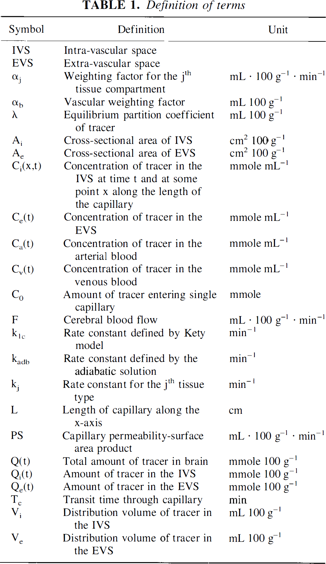
Using nonlinear regression analysis, the Kety equation (Equation 1) with the measured arterial concentration, C_a(t), is fitted to the tissue clearance data, Q(t), to obtain an estimate of k_1c. Cerebral blood flow can then be determined from k_1c using a known value of λ. (Herscovitch and Raichle, 1985).

Diffusion limitation of water

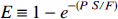
It has been demonstrated that water is not a freely diffusible tracer in the brain (Eichling et al., 1974), and as a result, the above relationship between F and k_1c has to be modified to include the extraction fraction (E) of water (Crone, 1963)

k_{l c} = \frac{E F}{λ}

(3)

where E represents the fraction of tracer that is extracted into the EVS during a single capillary transit. For modeling purposes, this fraction is assumed to attain an instantaneous diffusion equilibrium with the parenchymal tissue space (Kety, 1951). E is defined as (Crone, 1963)

E \equiv 1 - e^{- (P S / F)}

(4)

The Kety equation, after having been modified to include the extraction fraction of the tracer, becomes

Q (t) = E F \int_{0}^{t} C_{a} (t - u) e^{- k_{1 c} u} d u

(5)

where k_1c is now given by Equation 3.

There are two consequences to the diffusion limitation of water. First, because CBF is coupled with E, it is impossible to obtain an independent measurement of CBF from Equation 5 without knowing E. Depending on the magnitude of E, the underestimation of CBF can be significant if Equation 1 is used (Raichle et al., 1983). Second, Equation 5 does not account for the fact that the tracer (labeled water) requires a finite time to traverse the IVS. During this short time interval the entire amount of labeled water that enters at the arterial end of the capillary remains in the total tissue space (IVS and EVS). It has been demonstrated that the IVS tracer concentration can contribute to the signal and, if ignored, the CBF estimate may be time-dependent (Koeppe et al., 1987; Gambhir et al., 1987; Ohta et al., 1996).

Tissue homogeneity model

The TH model divides the brain into its two principal spaces: the IVS and the EVS, which are separated by the permeable blood—brain barrier (Johnson and Wilson, 1966; Sawada et al., 1989). Unlike the Kety model, the TH model defines the tracer concentration within the IVS as a function of both time and distance along the length of the capillary. Owing to the small radial dimension of a capillary radial concentration gradients can be neglected. Within the EVS, the tracer concentration is assumed to be homogeneous (i.e., well mixed) in its spatial distribution, and therefore, within this space the TH model is compartmental. The TH model represents a simplified version of the one-barrier distributed-parameter model described by Goresky et al. (1973) and Larson et al. (1987). It has been postulated by Sawada et al. (1989) that because of the high density of capillaries in the brain and their tortuous arrangement, it may be justifiable to treat the EVS as a compartment.

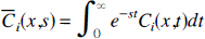
The capillary—tissue unit as defined by the TH model is illustrated in Fig. 1. From conservation of the mass of tracer in both the IVS and the EVS, the following equations can be derived

A_{i} \frac{\partial C_{i} (x, t)}{\partial t} = - F \frac{\partial C_{i} (x, t)}{\partial x} - \frac{P S}{L} [C_{i} (x, t) - \frac{C_{e} (t)}{λ}]

(6a)

A_{e} L \frac{d C_{e} (t)}{d t} = \frac{P S}{L} \int_{0}^{L} [C_{i} (x, t) - \frac{C_{e} (t)}{λ}] d x

(6b)

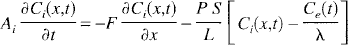
where all terms are defined in Table 1. These equations are subject to the following initial and boundary conditions

FIG. 1.

The capillary—tissue unit as assumed by the tissue homogeneity model. The model is comprised of an intravascular space (IVS) surrounded by an extravascular space (EVS). Both spaces are of equal length, L, measured along the x axis, which is the direction of flow. The two spaces are separated by the blood—brain barrier, which has a permeability—surface area product denoted by PS. Both spaces have an associated cross-sectional area, A_k, volume V_k, and tracer concentration C_k(t), where k = i or e. The model assumes that only the IVS tracer concentration is a function of position. Blood flows into the capillary—tissue unit by means of the arterial blood at a flow rate F and concentration C_a(t) and exits by means of the venous blood at the same flow rate and a concentration C_v(t).

\begin{aligned} C_{i} (x, t = 0) & = C_{e} (t) = 0 \\ C_{i} (x = 0, t > 0) & = C_{0} δ (t) \end{aligned}

(7)

The formal solution to Equation 6 is provided in the subsection entitled “Solution to the Tissue Homogeneity Model” in the appendix.

Adiabatic approximation to the tissue homogeneity model

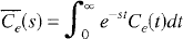
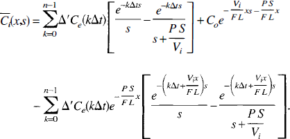
As shown in the appendix, the closed-form solution of the TH model exists only in Laplace space (Equations 23 and 24). In this section it is shown that an approximate closed-form solution in the time domain can be derived using the adiabatic approximation (Lassen and Perl, 1979). This approximation is motivated by the fact that the concentration of labeled water in the EVS (C_e(t)) changes slowly relative to that in the IVS (C_i(t)). Because of the difference in the time scale of these two events, for a small time interval, the slow event (i.e., the rate of change of C_e(t)) can be considered to be at a steady state while the fast event (i.e., the rate of change of C_i(t)) is taking place. The mathematical expression of the adiabatic approximation is to assume that within a small time increment (Δt), C_e(t) is constant. This assumption is justified in the brain since, for water, the ratio between its distribution volumes in the EVS and in the IVS is approximately 20:1 (Kety, 1951). Using the adiabatic assumption, C_e(t) becomes discrete and is given formally as

C_{e} (t) = \sum_{j = 0}^{n - 1} Δ C_{e} (j Δ t) u (t - j Δ t)

(8)

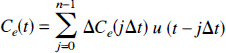
where ΔC_e(jΔt) is the discrete jump in the value of C_e(t) at time jΔt, and u(t) is the unit step function. A schematic diagram of this stepwise definition of C_e(t) is illustrated in Fig. 2. The adiabatic solution to the TH model is derived by substituting Equation 8 for C_e<(t) in the differential Equations governing mass conservation (Equations 6a and 6b). The complete derivation of this solution is presented in the subsection entitled “Adiabatic Approximation to the Tissue Homogeneity Model” in the appendix.

FIG. 2.

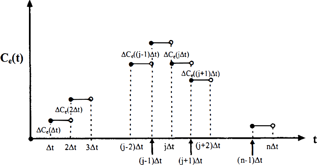
A schematic representation of the adiabatic approximation. This approximation states that C_e(t) can be represented by a staircase function because the EVS tracer concentration, C_e(t), changes slowly relative to the IVS concentration, C_i(x,t).

For the TH model, the impulse residue function (H(t)) (Zieler, 1965) derived from the adiabatic approximation is given by

H (t) = 1 0 ⩽ t < T_{c}

(9a)

H (t) = E e^{- \frac{E F}{V_{e}} (t - T_{C})} t ⩾ T_{c}

(9b)

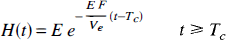
where T_c = V_i/F is the transit time through the capillary and E is defined by Equation 4.

By comparing Equation 9 to Equation 23 and 24, we have demonstrated that H(t) for the TH model can be greatly simplified by invoking the adiabatic approximation. With the adiabatic solution, H(t) is divided into two phases in the time domain. For the vascular phase (t < T_c), H(t) is equal to one owing to the finite time required for the labeled water to traverse the vascular space. During this phase, a fraction of the labeled water, denoted by E, is extracted into the EVS. At t = T_c, the remaining fraction (1 – E) exits by means of the outflowing blood, and hence there is a discrete drop in H(t). For t > T_c, which is the parenchymal tissue phase of H(t), the fraction of labeled water extracted into the EVS diffuses back into the IVS and is removed by blood flow, leading to clearance from the parenchymal tissue compartment (EVS).

As a corollary to the adiabatic approximation, because the time rate of change of the concentration of labeled water in the IVS owing to blood flow is much faster than that owing to diffusion, the capillary acts as a sink for the labeled water leaving the EVS (by diffusion) during the parenchymal tissue phase. The rate of change of the tracer concentration in the EVS, which for the TH model is considered a well-stirred compartment, can then be expressed as

V_{e} \frac{d C_{e} (t)}{d t} = - E F C_{e} (t)

(10)

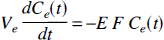
This equation has the same solution as derived for the TH model using the adiabatic approximation (Equation 9b). The product EF, as discussed by Renkin (1959) and Crone (1963), is the unidirectional flux of tracer from the EVS into the IVS.

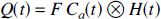
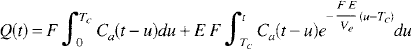
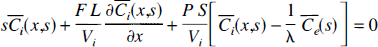
Figure 3 plots the exact solution and the adiabatic solution for the impulse residue function of the TH model at three different values of CBF: (1) 50 mL·100 g⁻¹·min⁻¹, (2) 100 mL·100 g⁻¹·min⁻¹, and (3) 200 mL·100 g⁻¹·min⁻¹ The values of V_i, V_e, and PS were 4.0 mL·100 g⁻¹, 94.0 mL·100 g⁻¹, and 150 mL·100 g⁻¹·min⁻¹, respectively (Herscovitch and Raichle, 1985; Herscovitch et al., 1987). In all three cases, the agreement between the exact model solution and the adiabatic approximation was excellent.

FIG. 3.

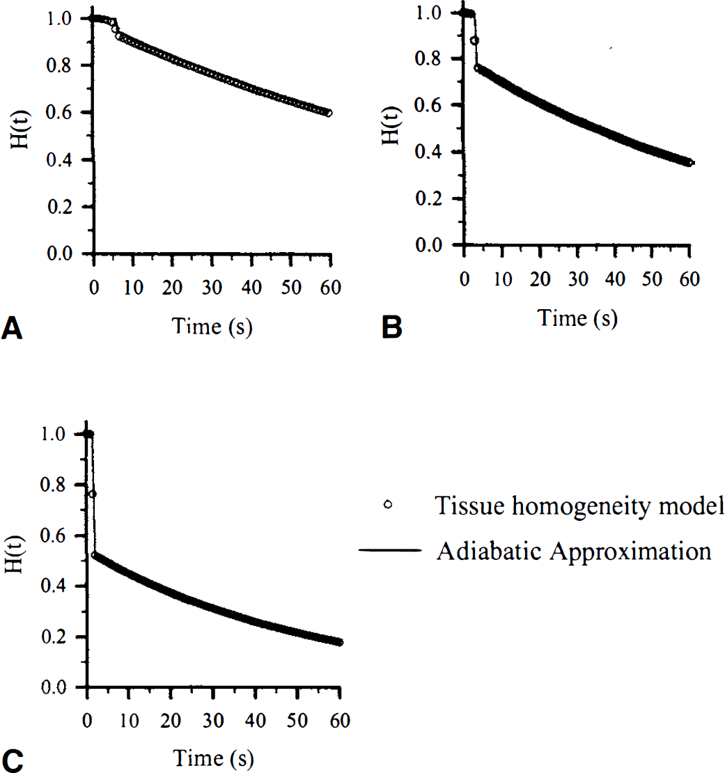
The impulse residue function, H(t), for the tissue homogeneity model as defined by the closed-form solution in the Laplace domain (Equations 23 and 24) compared with H(t) derived using the adiabatic solution (Equation 9). The comparison is illustrated for three cases: (A) CBF = 50 mL·100 g⁻¹·min⁻¹, (B) CBF = 100 mL·100 g⁻¹·min⁻¹ and (C) CBF = 200 mL·100 g⁻¹·min⁻¹. For all three cases shown, V_i;, V_e, and PS were 4.0 mL·100 g⁻¹, 94 mL·100 g⁻¹, and 150 mL·100 g⁻¹·min⁻¹, respectively.

Tissue residue curve

In CBF experiments, the tracer is often introduced at a peripheral site to avoid injection directly into a carotid artery. Under these conditions, the measured tissue residue curve Q(t) is the convolution of H(t) with an input curve C_a(t) (Zierler, 1965)

Q (t) = F C_{a} (t) \otimes H (t)

(11)

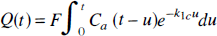
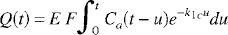
Inserting Equation 9 into Equation 11, Q(t) becomes

Q (t) = F \int_{0}^{T_{c}} C_{a} (t - u) d u + E F \int_{T_{c}}^{t} C_{a} (t - u) e^{- \frac{F E}{V_{e}} (u - T_{c})} d u

(12)

By introducing the change of variable u' = u – T_c in the second integral and by invoking the mean value theorem, Equation 12 can be written as

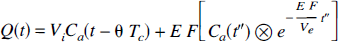
Q (t) = V_{i} C_{a} (t - θ T_{c}) + E F [C_{a} (t^{''}) \otimes e^{- \frac{E F}{V_{e}} t^{''}}]

(13)

where V_i = FT_c, t″ = t − T_c, and 0 ≤ θ ≤ 1. Since T_c is in the order of a few seconds (Larson et al., 1987), for t > T_c both C_a(t) and the convolution term in Equation 13 should change minimally in [(t – θT_c)t]; therefore, it is reasonable to approximate Equation 13 as

Q (t) = V_{i} C_{a} (t) + E F [C_{a} (t) \otimes e^{- k_{a d b} t}]

(14)

where the rate constant for the clearance of the tracer, k_adb, is defined as

k_{a d b} = \frac{E F}{V_{e}}

(15)

The assumption that T_c is equal to 0 is necessary if the tissue residue curve is sampled with a temporal resolution equal to or greater than T_c. In the next section, computer simulations were performed to determine the consequences of using this assumption. To determine CBF from Equation 14, both the concentration of labeled water in arterial blood and the concentration in brain tissue must be determined for a given time duration. A nonlinear regression algorithm is used to fit Equation 14 to the brain tissue data with three fitting parameters: (1) V_i, (2) the product EF, and (3) the rate constant k_adb.

In summary, using the adiabatic approximation, we derived a closed-form solution to the TH model in the time domain. This solution is similar to the Kety equation for a diffusion-limited tracer (Equation 5) except for two differences. First, the definition of the rate constant in the adiabatic solution involves V_e, whereas in the Kety equation, V_e is replaced by λ (Equation 3). In fact, V_e is equal to λ minus the distribution volume of water in the IVS, and therefore, these two parameters are similar in value in the brain. For example, in gray matter λ and V_e are equal to 98 and 94 mL·100 g⁻¹, respectively (Herscovitch and Raichle, 1985). Second and more important, the adiabatic solution includes a vascular phase term, V_iC_a(t), which accounts for the fact that during the transit time through the IVS (i.e., the vascular phase), the entire amount of tracer that enters by menas of the arterial input remains in the tissue (both IVS and EVS). At the end of the vascular phase, at t = T_c, a fraction of it, (1 – E), is removed by blood flow. It is the addition of the vascular phase term, V_iC_a(t), that we believe will eliminate the FFP that has been reported in the past (Ginsberg et al., 1982; Raichle et al., 1983).

Solutions to two-compartment models, which are similar to the adiabatic solution of the TH model, have previously been proposed to account for the vascular signal contribution (Gambhir et al., 1987; Ohta et al., 1996; Takagi et al., 1984). A limitation to modeling the IVS as a compartment is that the concentration is assumed to be uniform throughout the capillary. If the tracer exhibits any finite extraction, then it will continuously diffuse into the EVS during its passage from the arterial to the venous end of the capillary. As a result, there will be a concentration gradient from the arterial end to the venous end, and the assumption of a uniform capillary concentration is violated. It is interesting to note that although the TH model begins with a more realistic description of the exchange of water between the capillary and extravascular tissue, under the adiabatic approximation it reduces to a solution similar to that derived from compartmental analysis (Ohta et al., 1996). Therefore our derivation has shown the similarity between two-compartment models and the TH model in modeling transcapillary exchange in the brain.

METHODS

Accuracy of the adiabatic solution

The results presented in Fig. 3 demonstrated the excellent agreement between the closed-form solution in Laplace domain of the TH model (Equations 23 and 24) and the closed-form solution in the time domain derived using the adiabatic approximation (Equation 9). The final step taken to arrive at Equation 14 was to assume that for the case of a tissue residue curve sampled with time intervals greater than T_c, the mean transit time was zero. Computer simulations were used to determine whether this assumption was permissible over a wide range of CBF values. Simulated tissue residue data were generated using Equation 12 and a model arterial blood curve (Fig. 4). This arterial blood curve was determined by fitting a sum of three gamma variate functions to a representative set of arterial blood data from a D₂O washout experiment (see Part II). For all simulations, PS was 150 mL·100 g⁻¹·min⁻¹ (Herscovitch et al., 1987), and the volumes of the blood space and parenchymal tissue space were 4 and 94 mL·100 g⁻¹, respectively (Herscovitch and Raichle, 1985). Each simulated data set for Q(t) consisted of 900 data points with a sampling interval of 0.75 seconds for a total duration of 11.25 minutes. The simulated tissue data were generated over a range of flow values from 25 to 300 mL·100 g⁻¹·min⁻¹, and Equation 14 was fitted to the data using a quasi-Newton algorithm (Gill and Murray, 1974). Three fitting parameters were used in the analysis: (1) V_i, (2) the product EF, and (3) k_adb, as defined by Equation 15 because only one tissue type was simulated in these simulations.

FIG. 4.

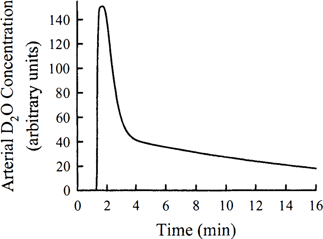
The model curve of arterial blood D₂O concentration versus time, which was used for all statistical error analysis. This curve was obtained by fitting a sum of three gamma variate functions to the set of experimental data from an experiment in Part II.

Error analysis

Noise, present in both the data for the concentration of D₂O in arterial blood and for the concentration of D₂O in tissue, will affect the precision of the estimated parameters. The influence of noise in the two data sets was investigated using both the covariance matrix (COV) method (Huang et al., 1986) and Monte Carlo computer simulations. The COV method was used for the noise analysis with the tissue data since the COV method was far less time-consuming than Monte Carlo computer simulations. However, the latter approach had to be used for the analysis of noise in the arterial blood data because the COV method could not account for noise in the input data. Since the two noise sources were uncorrelated in the experiments outlined in Part II, the total standard derivation associated with a parameter was equal to the standard deviations from both analyses added in quadrature.

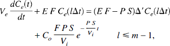
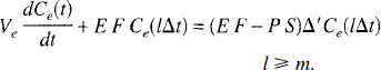
The error analysis was designed to reflect the ²H clearance experiments that are described in Part II. For these experiments, the adiabatic solution (Equation 14) was summed over two tissue types because the surface coil detected the ²H signal from both gray and white matter. The operational equation used in the simulations was as follows

Q (t) = \sum_{j = 1}^{2} α_{j} \int_{0}^{t} C_{a} (t - u) e^{- k_{j} u} d u + α_{b} C_{a} (t)

(16)

where α_j and k_j represented the weighting factor and the rate constant, respectively, for the jth tissue type (gray or white matter). The weighting factor was dependent on the product EF of the tissue type, as in Equation 14, the relative fraction, and the spatial sensitivity of the surface coil for the tissue type, as discussed in Part II. Note that the subscript adb was dropped from the rate constant since only its value was important for the error analysis and not its definition. The vascular phase terms for both tissue types had been lumped together as one (α_bC_a(t)). The parameter α_b depended on the vascular volume, the relative fraction, and the spatial sensitivity of the surface coil for each tissue type, similar to the case with α_j. In the ²H clearance experiments, it was not possible to cross-calibrate the two data sets (Q(t) and C_a(t)) owing to the nonuniformity of the spatial sensitivity of the surface coil. Therefore, in these experiments it was only the rate constant k_j that was related to CBF in the jth tissue compartment and not the weighting factor α_j. For this reason we focused our attention primarily on the rate constants in these simulations.

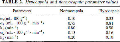
In the analysis of the ²H clearance data, a time shift (Δt) between the two data sets was included in the fitting routine to account for the difference between the arrival time of the labeled water in the brain and at the location at which the arterial blood was sampled. From a preliminary study we determined that including Δt as a fitting parameter had negligible effects on the precision and accuracy of the two rate constants. Since it was the rate constants that we were interested in, the parameter Δt was excluded from the error analysis. In summary, there were five regression parameters in the error analysis: two sets of α_j and k_j for gray and white matter, respectively, and α_b for the combined vascular phase terms of both gray and white matter. The SNR for each data set was defined as the maximum signal in a data set divided by the standard deviation of the background signal obtained from the spectra collected before D₂O injection (see Part II). The error analysis was performed using typical hypocapnia and normocapnia parameter values determined from the experiments described in Part II. These values are listed in Table 2, and the model arterial blood curve used in the analysis is illustrated in Fig. 4.

TABLE 2.

Hypocapnia and normocapnia parameter values

Parameters	Normocapnia	Hypocapnia
α_b(mL 100 g⁻¹)	0.10	0.03
α₁ (mL · 100 g⁻¹ · min⁻¹)	0.75	0.81
k₁ (min⁻¹)	0.80	0.50
α₂ (mL · 100 g⁻¹ · min⁻¹)	0.15	0.16
k₂ (min⁻¹)	0.20	0.10

Using the COV method, the coefficient of variation (CV) of each of the parameters listed in Table 2, was determined over a range of SNR (50 to 150) in the tissue data. Very briefly, the COV is defined as (Huang et al., 1986)

C O V = G^{- 1}

(17)

where G is the information matrix, and the (ij)th element of this matrix is given by

g_{i j} = \sum_{k} \frac{\partial Q (t_{k})}{\partial p_{i}} \cdot \frac{\partial Q (t_{k})}{\partial p_{i}} \cdot \frac{1}{{v a r}_{k}}

(18)

where p_i refers to the ith parameter, and var_k is the noise variance of Q(t_k). If the number of data points, Q(t_k), is large, then the diagonal terms of the COV approximate the variances of the parameter estimates. For this error analysis, Q(t) consisted of 300 samples with a sampling interval of 3 seconds, which was the data collection protocol used in the ²H clearance experiments.

In the ²H clearance experiments described in Part II, the data were also analyzed with the Kety equation summed over two tissue types to account for signals from both gray and white matter in the brain (Equation 16 without the α_bC_a(t) term). The purpose there was to investigate the FFP by comparing the results from the Kety equation to those from the adiabatic solution. In the present study, to compare the precision of the two rate constants determined from the Kety equation with those from the adiabatic solution, the above error analysis was repeated by excluding the α_bC_a(t) term in Equation 16. These simulations were only performed for the normocapnia values listed in Table 2. From this comparison, the effect of introducing the variable α_b on the precision of the two rate constants was determined.

For the simulations with noise included in the arterial blood data, a theoretical tissue residue curve was generated using Equation 16 with the parameter values listed in Table 2 and the model arterial blood curve (Fig. 4) at a temporal resolution of 3 seconds. For each simulation, an arterial data set was generated from the model arterial curve using the sampling protocol followed in the ²H clearance experiments described in Part II, which consisted of acquiring a sample every 6 seconds for the first 3.5 minutes, then every 12 seconds for the next 3 minutes, and finally every 30 seconds for the last 8.5 minutes. Noise was added to the arterial blood data, and before fitting Equation 16 to the theoretical tissue curve, the noisy arterial blood data set was interpolated to the same sampling interval as the tissue data. The Monte Carlo technique involved repeated simulations of the regression analysis with pseudorandom Gaussian noise added to the arterial data each time. The CV of each of the five parameters was determined from the distribution of estimated values generated from 500 simulations. The entire procedure was repeated for the same SNR range as was studied in the error analysis for noise in the tissue data.

Bias in the estimated parameters

Computer simulations were used to determine whether the correlation between the parameters could introduce a bias in the estimate of a parameter. The procedure for this study was analogous to the procedure for the simulations of noise in the arterial blood data except (1) the noise was added to the tissue data instead of the arterial blood data, (2) the SNR was maintained at 100, (3) simulations using the adiabatic solution (Equation 16) were generated only for the normocapnia parameters listed in Table 2, and (4) the simulations were performed for experimental durations of 4, 9, and 14 minutes. The same simulations were also conducted for the Kety equation summed over two tissue types. The only difference between the simulations for the Kety equation and those for the adiabatic solution was that the vascular phase term, α_b, in Equation 16 was set to zero for the former case. By comparing the results of the simulations for the adiabatic solution with the results for the Kety model, any bias introduced by a correlation between α_b and the rate constants will be evident since the simulations for the Kety model did not include α_b.

RESULTS

Accuracy of the adiabatic solution

The percent difference of the true values of the model parameters, EF and k_adb, from the estimated values, determined from regression analysis, is illustrated in Fig. 5A. For each parameter, the percent difference was plotted as a function of CBF. The estimated values of V_i from the regression analysis are presented in Fig. 5B. At all flow values investigated, the product EF was overestimated and V_i was consistently underestimated, both of which were attributed to setting T_c equal to 0 in Equation 13. To understand these results, it should be noted that the vascular phase term for the adiabatic solution originates from the integration of the arterial concentration of the tracer from time 0 to T_c. As well, the integration limits of the second term of Equation 12, which represents the fraction of labeled water extracted into parenchymal tissue, are from T_c to t. By forcing T_c to be 0, the fitting parameter V_i in Equation 14 could not account for the total area of the vascular phase term in Equation 12. Likewise, because the integration for the second term in Equation 14 is from 0 to t, EF therefore includes a portion of the vascular phase term in Equation 12. The accuracy of k_adb is not affected by this assumption because T_c does not contribute to the rate of tracer clearance from the EVS.

FIG. 5.

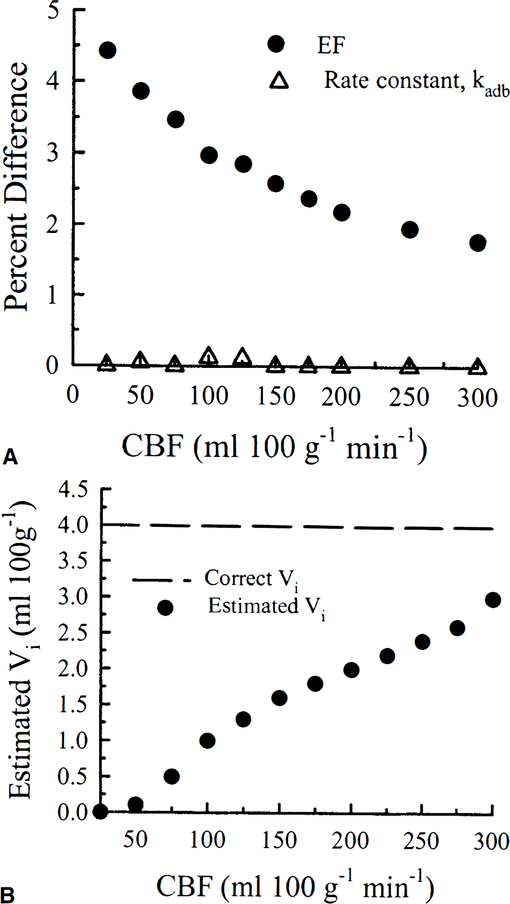
The effect on estimates of parameters in the adiabatic solution of the tissue homogeneity model by assuming that the mean transit time is equal to zero. (A) The percent error in the estimates of the model parameters, EF and k_adb, as a function of CBF. (B) Estimates of the parameter V_i as a function of CBF. All simulated tissue residue curves were generated using the arterial blood curve illustrated in Fig. 4 and the following values for the parameters V_i, V_e, and PS: 4.0 mL·100 g⁻¹, 94 mL·100 g⁻¹, and 150 mL·100 g⁻¹·min⁻¹, respectively.

Error analysis

Figure 6A illustrates the CV of the rate constant, k₁, of the higher flow tissue compartment (gray matter) as a function of SNR for four conditions: (1) hypocapnia with noise added to the tissue data, (2) hypocapnia with noise added to the arterial data, (3) normocapnia with noise added to the tissue data, and (4) normocapnia with noise added to the arterial data. The parameters for the hypocapnia and normocapnia simulations are given in Table 2. In Fig. 6B, the CV of the rate constant, k₂, of the lower flow tissue compartment (white matter) is plotted as a function of SNR for the same four conditions as for k₁. Because CBF was determined only from the rate constants, the CV of the other fitting parameters were not presented. The results in Fig. 6 indicated that the effect of noise in the arterial data was greater than that of the noise in the tissue data for the same SNR value. This difference could be attributed to the fact that fewer data points were acquired for the arterial data compared with the tissue data (70 versus 300, respectively).

FIG. 6.

(A) The coefficient of variation for k₁ plotted as a function of SNR. The parameter values used in the error analysis are listed in Table 2. Four different conditions are illustrated: (1) hypocapnia with noise added to the tissue data (dashed line with open triangles), (2) hypocapnia with noise added to the arterial data (dotted line with filled triangles), (3) normocapnia with noise added to the tissue data (solid line with open circles), and (4) normocapnia with noise added to the arterial data (dashed-dotted line with filled circles). (B) The CV for k₂ plotted as a function of SNR for the same four conditions as listed for k₁.

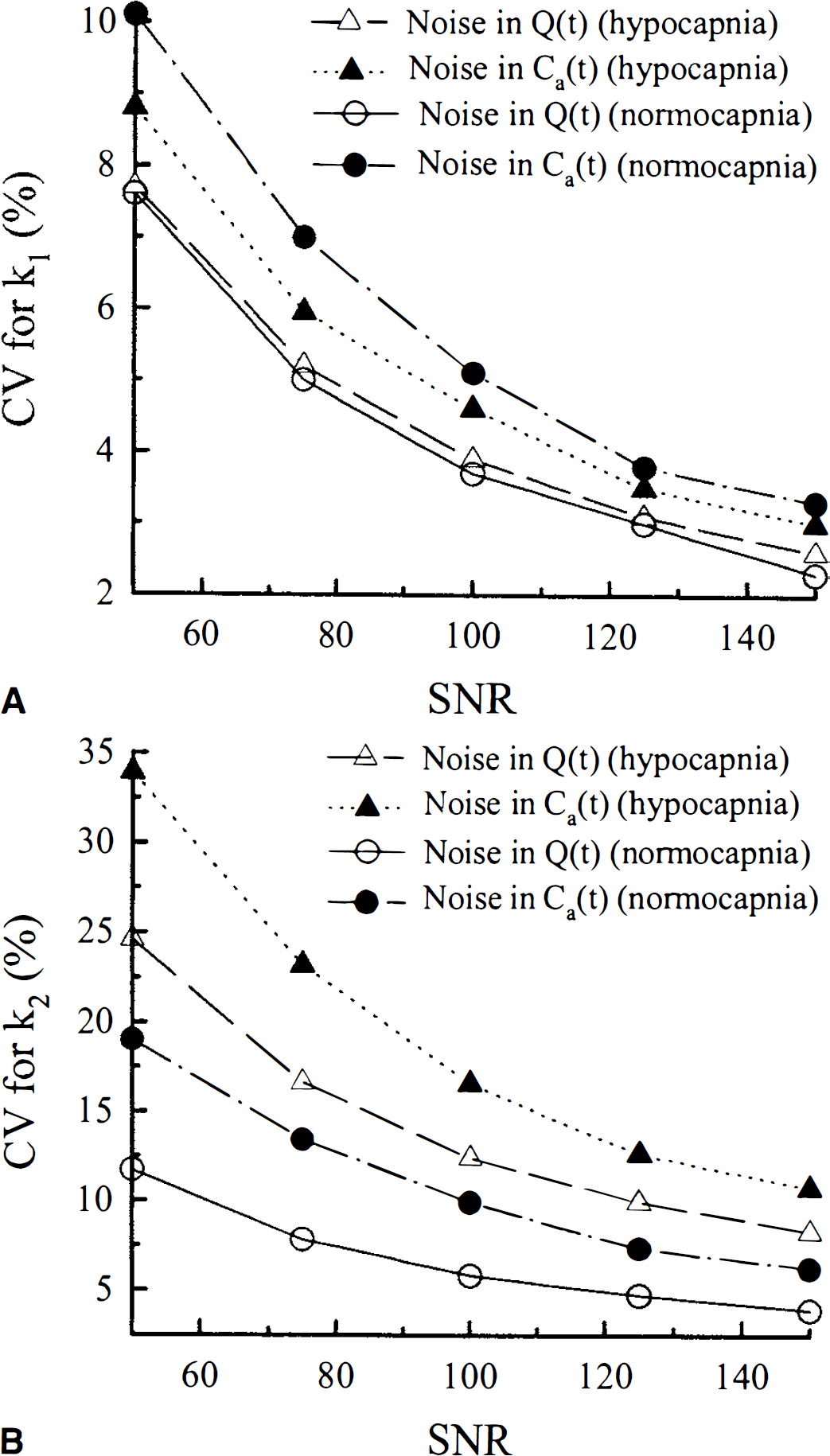
For all of the ²H clearance experiments, the SNR of the arterial blood data ranged from 70 to 100 and that of the tissue data was always greater than 120. For these SNR values, the CV of k₁ would be approximately 6% owing to noise in the arterial data and 3% owing to noise in the tissue data. If the standard deviations were assumed to add in quadrature, then the total CV of k₁ was 6.7%. The precision of k₂ was considerably worse than that of k₁. For the same SNR values, the CV of k₂ was roughly 20% for the arterial blood data and 10% for the tissue data, for a total CV of 22%. This reduction in the precision of k₂ was attributed to the smaller weighting factor for the second compartment. The importance of these precision estimates to the CBF measurements obtained with the ²H clearance technique will be addressed in the accompanying paper.

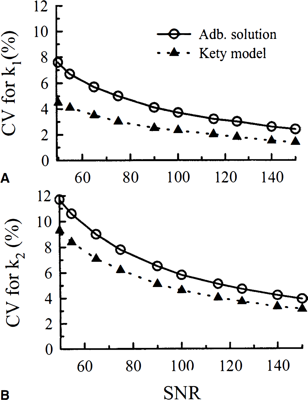
Besides the adiabatic solution simulations above, simulations involving the Kety equation were conducted to determine the decrease in precision that could be expected by including the additional term α_b in the regression analysis. In Fig. 7, the CV for k₁ and k₂ are presented for both the adiabatic solution and the Kety equation summed over two tissue types. These simulations included only noise in the tissue data. As shown in these figures, including α_b resulted in an increase of no greater than 3% for the CV of either rate constant over the entire range of SNR values studied.

FIG. 7.

(A) The CV for k₁ plotted as a function of tissue data SNR. The CV is presented for both the adiabatic solution of the TH model and the Kety model solution. These results were generated using the parameter values listed in Table 2 for the normocapnia case. (B) The corresponding CV for k₂ plotted as a function of the tissue data SNR.

Bias in the estimated parameters

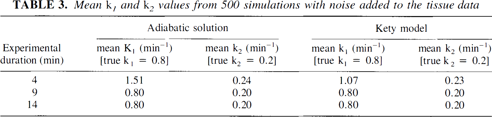
In Table 3, the mean k₁ and k₂ values from 500 simulations with noise added to the tissue data are listed. The results of the simulations of both the Kety equation and the adiabatic solution for three different experimental durations, 4, 9, and 14 minutes, were presented, The true values of k₁ and k₂ were the normocapnia values listed in Table 2. These results indicated that when only the first 4 minutes of the data were included in the regression analysis, both rate constants were overestimated with either the Kety model or the adiabatic solution, Furthermore, this bias was more pronounced with the higher rate constant, k₁, than with the lower rate constant, k₂. The bias was significantly larger for the adiabatic solution, which was attributed to the correlation between α_b and k₁. By increasing the experimental duration to 9 minutes, this correlation was sufficiently reduced such that the bias in k₁ was eliminated. With the Kety equation, the bias was not nearly as large simply because of the absence of α_b. The small bias associated with the Kety model was attributed to the constraints imposed on the fitting parameters in the regression analysis.

DISCUSSION

In this study it was demonstrated that a time-domain, closed-form solution to the TH model can be derived using the adiabatic approximation. The consequences of this derivation are twofold. First, the adiabatic solution can be easily implemented in the analysis of clearance data because the solution is in the time domain. Furthermore, considering that there are only three fitting parameters (V_i, EF, and k_adb) in the model for each tissue type, it can be used to analyze clearance data of limited time resolution or SNR, or both. Examples of such applications include dynamic positron emission tomography studies with the tracer H₂¹⁵O (Alpert et al., 1984) and magnetic resonance spectroscopy using the tracer D₂O (Kim and Ackerman, 1990). Second, the similarity between the adiabatic solution and the solutions derived from two-compartment models indicates that the use of two-compartment models is reasonable provided that the vascular phase of the signal is properly accounted for in the models.

Using computer simulations, the accuracy of the adiabatic solution (Equation 14) was investigated over a wide range of CBF values (25 to 300 mL·100 g⁻¹·min⁻¹). It was determined that the assumption T_c = 0 results in a consistent underestimation of V_i and an overestimation of EF; however k_adb remains unaffected. These results are significant for two reasons. First, the accuracy of the CBF measurements presented in Part II was not compromised by this approximation since CBF was determined from k_adb only. Second, these findings suggest that the measured product EF could not be considered to represent only water clearance from the EVS (Ohta et al., 1996), since this parameter might be overestimated for reasons discussed in the Results section. However, this overestimation would not be as large as when the vascular phase term is ignored completely (Ohta et al., 1996). Finally, the assumption that T_c is equal to zero is only necessary to accommodate clearance data collected with limited temporal resolution. If the data are acquired with sufficient temporal resolution (i.e., sampling interval less than T_c), then T_c can be included as a fitting variable in the regression analysis, which will avoid these errors.

Although the results illustrated in Fig. 3 clearly demonstrated the validity of the adiabatic solution to the TH model, they were only generated for parameter values that reflect water transport in the brain. If another tracer is used or a different tissue studied, then it may be necessary to reevaluate the adiabatic solution under those specific conditions. Furthermore, the ability of the adiabatic solution to properly characterize tracer transport through the microvasculature depends on the validity of the TH model in representing the tissue studied. The variability of the microvascular architecture from one tissue type to another is considerable, and for some tissues, the representation of the EVS as a well-stirred compartment, as in the TH model, may not be valid. For instance, the highly ordered arrangement of the capillaries in the liver would mean that the EVS can not be represented by a compartment. It has been suggested that the TH model may not even be appropriate for characterizing water exchange in the brain (Kassissia et al., 1995), which in turn would cast doubt on the validity of the adiabatic solution. We have tested the validity of the adiabatic solution by measuring CBF in rabbit brain using magnetic resonance spectroscopy with the tracer D₂O and demonstrated that the TH model is valid for brain tissue. The results of this study will be presented in Part II.

TABLE 3.

Mean k_j and k₂ values from 500 simulations with noise added to the tissue data

	Adiabatic solution		Kety model
Experimental duration (min)	mean K₁ (min⁻¹) [true k₁ = 0.8]	mean k₂ (min⁻¹) [true k₂ = 0.2]	mean k₁ (min⁻¹) [true k₁ = 0.8]	mean k₂ (min⁻¹) [true k₂ = 0.2]
4	1.51	0.24	1.07	0.23
9	0.80	0.20	0.80	0.20
14	0.80	0.20	0.80	0.20

As well as determining the accuracy of the adiabatic solution, the precision of the estimated model parameters was also investigated for the specific conditions of the experiments outlined in Part II. The error analysis involved summing the adiabatic solution over two tissue types because in the CBF experiments, the ²H signal originated from both gray and white matter in the brain. Accounting for both tissue types greatly increased the demands on the SNR and the temporal resolution of the data. The results plotted in Fig. 6 demonstrated that the precision of the higher rate constant of the gray matter was acceptable. However, the precision of the lower rate constant of the white matter was poor because of its smaller weighting factor. By including the vascular phase term, α_b, in the regression analysis, a maximum of only 3% increase in the CV for either rate constant was determined. Therefore, the limiting factor for precision in the experimental protocol was summing the operational equation over two tissue types and not including α_b. Although α_b did not greatly increase the CV of either rate constant, it did introduce a bias in their estimated values, which was especially prominent for k₁. However, the correlation between these parameters could be eliminated by increasing the experimental duration to greater than 9 minutes. As a result, for the CBF experiments discussed in Part II the time duration was chosen to be 15 minutes.

APPENDIX

Solution to the tissue homogeneity model

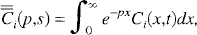
The formal solution to Equation 6 is obtained by using the Laplace transform. The transformed functions are denoted by a bar.

{\bar{C}}_{i} (x, s) = \int_{0}^{\infty} e^{- s t} C_{i} (x, t) d t

(19)

\bar{C_{e}} (s) = \int_{0}^{\infty} e^{- s t} C_{e} (t) d t

(20)

In terms of the transformed functions, Equations 6a and 6b can be rewritten as

s \bar{C_{i}} (x, s) + \frac{F L}{V_{i}} \frac{\partial {\bar{C}}_{i} (x, s)}{\partial x} + \frac{P S}{V_{i}} [\bar{C_{i}} (x, s) - \frac{1}{λ} \bar{C_{e}} (s)] = 0

(21)

V_{e} s \bar{C_{e}} (s) - \frac{P S}{L} \int_{0}^{L} \bar{C_{i}} (x, s) d x - \frac{P S}{λ} \bar{C_{e}} (s) = 0

(22)

The solutions of these equations are (Johnson and Wilson, 1966)

\bar{C_{i}} (x, s) = \frac{C_{0}}{s} e^{- (α + β s) x / L} + \frac{[1 - e^{- (α + β s)} I 1 - e^{- (α + β s) x / L}]}{s [U (s) - e^{- (α + β s)}]}

(23)

\bar{C_{i}} (s) = \frac{λ (α + β s) [1 - e^{- (α + β s)}]}{α β s [U (s) - e^{- (α + β s)}]}

(24)

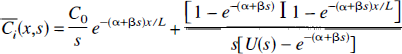
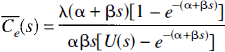
where U(s), a cubic polynomial in seconds, and the three variables, α, β, and χ, are defined as

\begin{aligned} U (s) & = \frac{χ}{α^{2}} (β s)^{3} + \frac{(2_{χ} + 1)}{α} (β s)^{2} + (χ + 1) β s + 1 \\ α & = \frac{P S}{F}, β = \frac{V_{i}}{F}, χ = \frac{V_{e}}{V_{i}} λ \end{aligned}

(25)

Adiabatic approximation to the tissue homogeneity model

To solve the mass conservation equations (Equations 6a and 6b) using the adiabatic approximation, we begin with the differential equation for the IVS. First, by Laplace transform with respect to time, Equation 6a can be written as follows

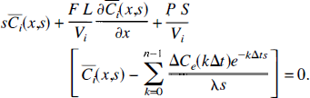
\begin{aligned} s \bar{C_{i}} (x, s) + & \frac{F L}{V_{i}} \frac{\partial \bar{C_{i}} (x, s)}{\partial x} + \frac{P S}{V_{i}} \\ [\bar{C_{i}} (x, s) - \sum_{k = 0}^{n - 1} \frac{Δ C_{e} (k Δ t) e^{- k Δ t s}}{λ s}] = 0. \end{aligned}

(26)

where the discrete version of C_e(t), Equation 8, has been used. Next, Laplace transform with respect to position is performed by using the definition

{\overset{=}{C}}_{i} (p, s) = \int_{0}^{\infty} e^{- p x} C_{i} (x, t) d x,

(27)

where the double bar notation refers to the two Laplace transforms with respect to the variables x and t. The Laplace transform of Equation 26 with respect to position is

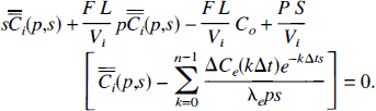
\begin{aligned} s {\overset{=}{C}}_{i} (p, s) + & \frac{F L}{V_{i}} p {\overset{=}{C}}_{i} (p, s) - \frac{F L}{V_{i}} C_{o} + \frac{P S}{V_{i}} \\ [{\overset{=}{C}}_{i} (p, s) - \sum_{k = 0}^{n - 1} \frac{Δ C_{e} (k Δ t) e^{- k Δ t s}}{λ_{e} p s}] = 0. \end{aligned}

(28)

This equation is obtained using the boundary conditions stated in Equation 7. Performing the inverse Laplace transform with respect to p, we obtain the following equation

\begin{aligned} {\bar{C}}_{i} (x, s) = & \sum_{k = 0}^{n - 1} Δ^{'} C_{e} (k Δ t) [\frac{e^{- k Δ t s}}{s} - \frac{e^{- k Δ t s}}{s + \frac{P S}{V_{i}}}] + C_{o} e^{- \frac{V_{i}}{F L} x s - \frac{P S}{F L} x} \\ - & \sum_{k = 0}^{n - 1} Δ^{'} C_{e} (k Δ t) e^{- \frac{P S}{F L} x} [\frac{e^{- (k Δ t + \frac{V_{i} x}{F L}) s}}{s} - \frac{e^{- (k Δ t + \frac{V_{i} x}{F L}) s}}{s + \frac{P S}{V_{i}}}] . \end{aligned}

(29)

In Eq. (29), we have made the substitution $\frac{Δ C_{e} (k Δ t)}{λ} = Δ^{'} C_{e} (k Δ t)$ . Next we perform the inverse Laplace transform with respect to t:

\begin{aligned} C_{i} (x, t) = & \sum_{k = 0}^{n - 1} Δ^{'} C_{e} (k Δ t) u (t - k Δ t) \\ - \sum_{k = 0}^{n - 1} Δ^{'} C_{e} (k Δ t) e^{- \frac{P S}{V_{i}} (t - k Δ t)} u (t - k Δ t) \\ - \sum_{k = 0}^{n - 1} Δ^{'} C_{e} (k Δ t) e^{- \frac{P S}{F L} x} u (t - k Δ t - \frac{V_{i} x}{F L}) \\ + \sum_{k = 0}^{n - 1} Δ^{'} C_{e} (k Δ t) e^{- \frac{P S}{F L} x} u (t - k Δ t - \frac{V_{i} x}{F L}) \\ e^{- \frac{P S}{V_{b}} (t - k Δ t - \frac{V_{i} x}{F L})} + C_{o} e^{- \frac{P S}{F L} x} δ (t - \frac{x}{v}), \end{aligned}

(30)

where: $v = \frac{F L}{V_{i}}$ .

Now consider one of the Δt intervals in [0,nΔt), say t ∊ [lΔt,(l + 1)Δt), where 0 ≤ l ≤ (n = 1). After some simplification Equation 30 becomes

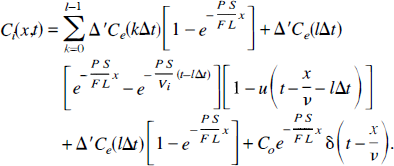
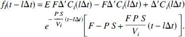
\begin{aligned} C_{i} (x, t) = & \sum_{k = 0}^{l - 1} Δ^{'} C_{e} (k Δ t) [1 - e^{- \frac{P S}{F L} x}] + Δ^{'} C_{e} (l Δ t) \\ [e^{- \frac{P S}{F L} x} - e^{- \frac{P S}{v_{i}} (t - l Δ t)}] [1 - u (t - \frac{x}{v} - l Δ t)] \\ + Δ^{'} C_{e} (l Δ t) [1 - e^{- \frac{P S}{F L} x}] + C_{o} e^{- \frac{P S}{F L} x} δ (t - \frac{x}{v}) . \end{aligned}

(31)

The next step is to integrate this equation over the length of the capillary to determine the amount of tracer in the IVS

Q_{i} (l Δ_{t}) = {[A_{i} \int_{0}^{L} C_{i} (x, t) d x]}_{t = l Δ_{t}} .

(32)

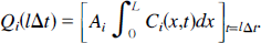
Using Equation 31 to define C_i(x,t), we obtain the following

\begin{aligned} Q_{i} (l Δ t) = & V_{i} C_{e} ((l - 1) Δ t) - \frac{E F}{P S} V_{i} C_{e} ((l - 1) Δ t) + C_{o} F e^{- \frac{P S}{V_{i}} l Δ t} \\ 1 ⩽ l ⩽ m - 1 \end{aligned}

(33)

\begin{aligned} Q_{i} (l Δ t) = & V_{i} C_{e} ((l - 1) Δ t) - \frac{E F}{P S} V_{i} C_{e} ((l - 1) Δ t) \\ m ⩽ l ⩽ n - 1, \end{aligned}

(34)

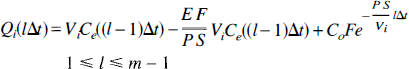
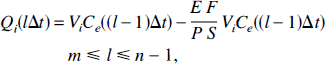
for t ∊ [lΔt, (l + 1)Δt), where $C_{e} (l Δ t) = \sum_{k = 0}^{l} Δ^{'} C_{E} (k Δ t)$ and $m Δ t = \frac{L}{v}$ . In Eq. (A.12) the term E represents the extraction fraction of tracer as defined by Eq. (4).

With the tracer amount in the IVS known, the next step is to determine the tracer concentration in the EVS. Using Equation 31, the differential equation for tracer mass conservation in the EVS (Equation 6b) becomes

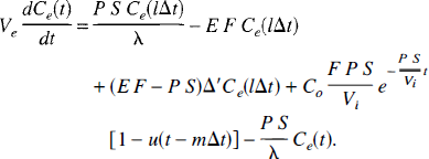
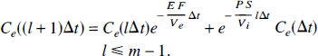
\begin{aligned} V_{e} \frac{d C_{E} (t)}{d t} = & \frac{P S C_{e} (l Δ t)}{λ} - E F C_{e} (l Δ t) \\ + (E F - P S) Δ^{'} C_{e} (l Δ t) + C_{o} \frac{F P S}{V_{i}} e^{- \frac{P S}{V_{i}} t} \\ [1 - u (t - m Δ t)] - \frac{P S}{λ} C_{e} (t) . \end{aligned}

(35)

With the adiabatic approximation for C_e(t), we could assume C_e(lΔt) ≈ C_e(t) for t ∊ [lΔt,(l + 1)Δt), and hence Equation 35 becomes

\begin{aligned} V_{e} \frac{d C_{e} t}{d t} & + E F C_{e} (l Δ t) = (E F - P S) Δ^{'} C_{e} (l Δ t) \\ + C_{o} \frac{F P S}{V_{i}} e^{- \frac{P S}{V_{i}} t} l ⩽ m - 1, \end{aligned}

(36)

\begin{aligned} V_{e} \frac{d C_{e} t}{d t} + E F C_{e} (l Δ t) = (E F & - P S) Δ^{'} C_{e} (l Δ t) \\ l ⩾ m . \end{aligned}

(37)

Equation 36 has the solution

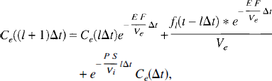
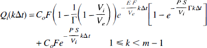
\begin{aligned} C_{e} ((l + 1) Δ t) = & C_{e} (l Δ t) e^{- \frac{E F}{V_{e}} Δ t} + \frac{f_{l} (t - l Δ t) * e^{- \frac{E F}{V_{e}} Δ t}}{V_{e}} \\ + e^{- \frac{P S}{V_{i}} l Δ t} C_{e} (Δ t), \end{aligned}

(38)

where * denotes the convolution operator and the factor f₁ is defined as

\begin{aligned} f_{l} (t - l Δ t) = & E F Δ^{'} C_{i} (l Δ t) - F Δ^{'} C_{i} (l Δ t) + Δ^{'} C_{i} (l Δ t) \\ e^{- \frac{P S}{V_{i}} (t - l Δ t)} [F - P S + \frac{F P S}{V_{i}} (t - l Δ t)] . \end{aligned}

(39)

For an infinitesimally small Δt, the convolution will approach zero and thus Equation 38 reduces to

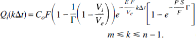
\begin{aligned} C_{e} ((l + 1) Δ t) = & C_{e} (l Δ t) e^{- \frac{E F}{V_{e}} Δ t} + e^{- \frac{P S}{V_{i}} l Δ t} C_{e} (Δ t) \\ l ⩽ m - 1. \end{aligned}

(40)

Similarly, the solution to Equation 37 is

C_{e} ((l + 1) Δ t) = C_{e} (l Δ t) e^{- \frac{E F}{V_{e}} Δ t} l ⩾ m .

(41)

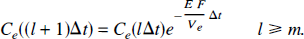
From these recursive relationships, Equations 40 and 41, it can be shown that for any interval k the EVS concentration is given by

\begin{aligned} C_{e} (k Δ t) = & \frac{C_{o} F e^{- \frac{E F}{V_{e}} k Δ t}}{V_{e} Γ} [1 - e^{- \frac{P S}{V_{i}} Γ k Δ t}] \\ 0 ⩽ k < m - 1 \end{aligned}

(42)

\begin{aligned} C_{e} (k Δ t) = & \frac{C_{o} F e^{- \frac{E F}{V_{e}} k Δ t}}{V_{e} Γ} [1 - e^{- \frac{P S}{F} Γ}] \\ m ⩽ k < m - 1, \end{aligned}

(43)

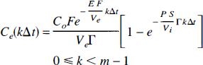
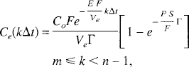
where $Γ = 1 - \frac{E F}{P S} \frac{V_{i}}{V_{e}}$ .

Using Equations 42 and 43 to define the EVS concentration, the amount of tracer in the IVS can be determined from Equations and 33 and 34.

\begin{aligned} Q_{i} (k Δ t) = & C_{o} F (1 - \frac{1}{Γ} (1 - \frac{V_{i}}{V_{e}})) e^{- \frac{E F}{V_{e}} k Δ t} [1 - e^{- \frac{P S}{V_{i}} Γ k Δ t}] \\ C_{o} F e^{- \frac{P S}{V_{i}} k Δ t} 1 ⩽ k < m - 1 \end{aligned}

(44)

\begin{aligned} Q_{i} (k Δ t) = & C_{o} F (1 - \frac{1}{Γ} (1 - \frac{V_{i}}{V_{e}})) e^{- \frac{E F}{V_{e}} k Δ t} [1 - e^{- \frac{P S}{V_{i}} Γ}] \\ m ⩽ k ⩽ n - 1. \end{aligned}

(45)

The total amount of tracer in the brain volume is given by

Q (t) = V_{e} C_{e} (t) + Q_{i} (t) .

(46)

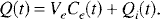
From Equations 42, 43, 44, and 45, Q(t) is

\begin{aligned} Q (k Δ t) = & C_{o} F (1 + \frac{V_{i}}{Γ V_{e}}) e^{- \frac{E F}{V_{e}} k Δ t} [1 - e^{- \frac{P S}{V_{i}} Γ k Δ t}] \\ C_{o} F e^{- \frac{P S}{V_{i}} k Δ t} 1 ⩽ k < m - 1 \end{aligned}

(47)

\begin{aligned} Q (k Δ t) = & C_{o} F (1 + \frac{V_{i}}{Γ V_{e}}) e^{- \frac{E V_{i}}{V_{e}}} [1 - e^{- \frac{P S}{F} Γ}] e^{- \frac{E F}{V_{e}} (k - m) Δ t} \\ m ⩽ k ⩽ n - 1. \end{aligned}

(48)

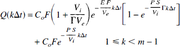
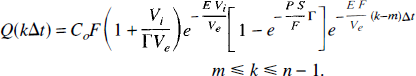
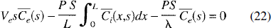
These equations can be simplified considerably by making the folowing assumptions: (i) Γ ∼ 1 since E F V_i ≪ P S V_e, (ii) in Eq. (47) $e^{\frac{E F}{V_{e}} k Δ t} \sim 1$ since kΔt is less than or equal to the capillary transit time, and (iii) in Eq. (A.48) $e^{- \frac{E V}{V_{e}}} \sim 1$ since V_e ≫ E V_i. Therefore.

\begin{aligned} (1 + \frac{V_{i}}{Γ V_{e}}) e^{- \frac{E F}{V_{e}} k Δ t} & [1 - e^{- \frac{P S}{V_{i}} Γ k Δ t}] + e^{- \frac{P S}{V_{i}} k Δ t} \approx 1 \\ 1 ⩽ k < m - 1 \end{aligned}

(49)

\begin{aligned} (1 + \frac{V_{i}}{Γ V_{e}}) e^{- \frac{E V_{i}}{V_{e}}} & [1 - e^{- \frac{P S}{F} Γ}] \approx [1 - e^{- \frac{P S}{F}}] \\ m ⩽ k ⩽ n - 1. \end{aligned}

(50)

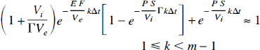
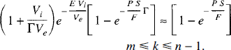
To demonstrate the validity of these approximations, the terms on the left side of Equations 49 and 50 and their respective approximate solutions (the right side of the equations) are plotted as functions of CBF in Fig. 8. For these curves, values of V_i, V_e, and PS are chosen that represent typical values for water transport in brain: 4.0 mL·100 g⁻¹, 94.0 mL·100 g⁻¹, and 150 mL·100 g⁻¹·min⁻¹, respectively (Herscovitch and Raichle, 1985; Herscovitch et al., 1987). Equation 49 is plotted for a transit time of 3 seconds, which represents the mean vascular transit time in brain (Larson et al., 1987). The impulse residue function, H(t), is obtained by setting C₀F equal to 1 in Equations 47 and 48 and using the approximations given in Equations 49 and 50. The final form of H(t) is shown in Equations 9a and 9b in the theory section.

FIG. 8.

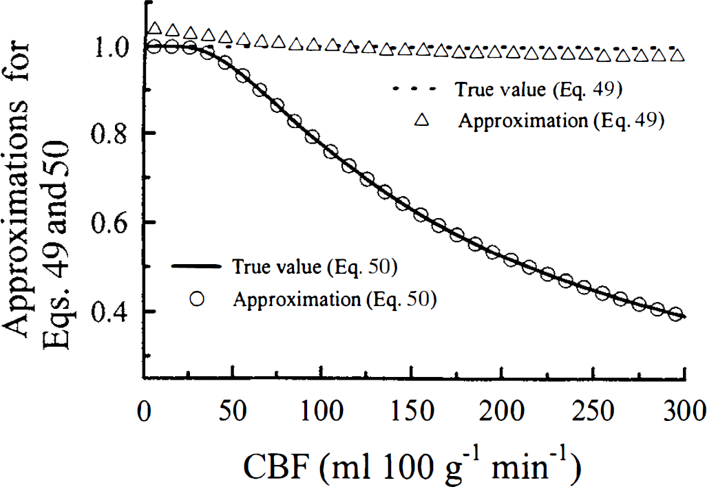
Graphical representation of the approximations given by Equations 49 and 50 plotted as a function of CBF. For all calculations, V_i, V_e, and PS were 4.0 mL·100 g⁻¹ 94.0 mL·100 g⁻¹, and 150 mL·100 g⁻¹·min⁻¹, respectively. Equation 49 was plotted for a transit time of 3 seconds.

Footnotes

Abbreviations used

References

Alpert

Eriksson

Chang

Bergstrom

Litton

Correia

Bohm

Ackerman

Taveras

(1984) Strategy for the measurement of regional cerebral blood flow using short-lived tracers and emission tomography. J Cereb Blood Flow Metab 4: 28–34

Corbett

RJT

Laptook

Olivares

(1991) Simultaneous measurement of cerebral blood flow and energy metabolites in piglets using deuterium and phosphorus nuclear magnetic resonance. J Cereb Blood Flow Metab 11: 55–65

Crone

(1963) The permeability of capillaries in various organs as determined by use of the ‘indicator diffusion’ method. Acta Physiol Scand 58:292–305

Detre

Subramanian

Mitchell

Smith

Kobayashi

Zaman

Leigh

(1990) Measurement of regional cerebral blood flow in cat brain using intracarotid ²H₂O and ²H NMR imaging. Magn Reson Med 14:389–395

Eichling

Grubb

Jr Raichle

Ter-Pogossian

(1974) Evidence of the limitations of water as a freely diffusable tracer in brain of the rhesus monkey. Circulation Res 35:358–364

Frackowiak

RSJ

Lenzi

G-L

Jones

Heather

(1980) Quantitative measurement of regional cerebral blood flow and oxygen metabolism in man using O-15 and positron emission tomography: theory, procedure, and normal values. J Comput Assist Tomogr 4:727–736

Gambhir

Huang

S-C

Hawkins

Phelps

(1987) A study of the single compartment tracer kinetic model for the measurement of local cerebral blood flow using ¹⁵O-water and positron emission tomography. J Cereb Blood Flow Metab 7:13–20

Gill

Murray

(1974) Numerical Methods for Constrained Optimization, London, Academic Press

Ginsberg

Lockwood

Busto

Finn

Bulter

Cendan

Goddard

(1982) A simplified in vivo autoradiographic strategy for the determination of regional cerebral blood flow by positron emission tomography: theoretical considerations and validation studies in the rat. J Cereb Blood Flow Metab 2:89–98

10.

Goresky

Bach

Nadeau

(1973) On the uptake of materials by the intact liver. The transport and net removal of galactose. J Clin Invest 52:991–1009

11.

Herscovitch

Raichle

(1985) What is the correct value for the brain—blood partition coefficient for water? J Cereb Blood Flow Metab 5:65–69

12.

Herscovitch

Raichle

(1987) Positron emission tomographic measurement of cerebral blood flow and permeability—surface area product of water using [¹⁵O] water and [¹¹C]butanol. J Cereb Blood Flow Metab 7:527–542

13.

Huang

S-C

Carson

Phelps

(1982) Measurement of local blood flow and distribution volume with short-lived isotopes: a general input technique. J Cereb Blood Flow Metab 2:99–108

14.

Huang

S-C

Feng

Phelps

(1986) Model dependency and estimation reliability in measurement of cerebral oxygen utilization rate with oxygen-15 and dynamic positron emission tomography. J Cereb Blood Flow Metab 6: 105–119

15.

Johnson

Wilson

(1966) A model for capillary exchange. Am J Physiol 210:1299–1303

16.

Kassissia

Goresky

Rose

Schwab

Simard

Huet

P-M

Bach

(1995) Tracer oxygen distribution is barrier-limited in the cerebral microcirculation. Circ Res 77:1201–1211

17.

Kety

(1951) The theory and application of the exchange of inert gas at the lungs and tissues. Pharmacol Rev 3:1–41

18.

Kim

S-G

Ackerman

JJH

(1990) Quantification of regional blood flow by monitoring of exogenous tracer via nuclear magnetic resonance spectroscopy. Magn Reson Med 14:266–282

19.

Koeppe

Hutchins

Rothley

Hichwa

(1987) Examination of assumptions for local cerebral blood flow studies in PET. J Nucl Med 28:1695–1703

20.

Larson

Markham

Raichle

(1987) Tracer-kinetic models for measuring cerebral blood flow using detected radiotracers. J Cereb Blood Flow Metab 7:443–463

21.

Lassen

Perl

(1979) Tracer Kinetic Methods in Medical Physiology, New York, Raven Press, p 168

22.

Ohta

Meyer

Fujita

Reutens

Evan

Gjedde

(1996) Cerebral [¹⁵O]water clearance in humans determined by PET: I. theory and normal values. J Cereb Blood Flow Metab 16:765–780

23.

Pekar

Ligeti

Ruttner

Lyon

Sinnwell

Van Gelderen

Fiat

Moonen

CTW

McLaughlin

(1991) In vivo measurement of cerebral oxygen consumption and blood flow using ¹⁷O magnetic resonance imaging. Magn Reson Med 21:313–319

24.

Quarles

Mintun

Larson

Markham

MacLeod

Raichle

(1993) Measurement of regional cerebral blood flow with positron emission tomography: a comparison of [¹⁵O]water to [¹¹C]butanol with distributed-parameter and compartmental models. J Cereb Blood Flow Metab 13:733–747

25.

Raichle

Martin

WRW

Herscovitch

Mintun

Markham

(1983) Brain blood flow measured with intravenous H₂ ¹⁵O. II. Implementation and validation. J Nucl Med 24:790–798

26.

Renkin

(1959) Transport of potassium-42 from blood to tissue in isolated mammalian skeletal muscles. Am J Physiol 197:1205–1210

27.

Sawada

Patlak

Blasberg

(1989) Kinetic analysis of cerebrovascular transport based on indicator diffusion technique. Am J Physiol 256:H794–H812

28.

Takagi

Kenny

Gilson

(1984) A quantitative model for the measurement of cerebral vascular extraction fraction in vivo following intravenous injection: simulation studies. J Cereb Blood Flow Metab 4:564–573

29.

Williams

Detre

Leigh

Koretsky

(1992) Magnetic resonance imaging of perfusion using spin inversion of arterial water. Proc Natl Acad Sci USA 89:212–216

30.

Zieler

(1965) Equations for measuring blood flow by external monitoring of radioisotopes. Circ Res 16:309–321

An Adiabatic Approximation to the Tissue Homogeneity Model for Water Exchange in the Brain: I. Theoretical Derivation

Abstract

Keywords

THEORY

Kety model

Diffusion limitation of water

Tissue homogeneity model

Adiabatic approximation to the tissue homogeneity model

Tissue residue curve

METHODS

Accuracy of the adiabatic solution

Error analysis

Bias in the estimated parameters

RESULTS

Accuracy of the adiabatic solution

Error analysis

Bias in the estimated parameters

DISCUSSION

APPENDIX

Solution to the tissue homogeneity model

Adiabatic approximation to the tissue homogeneity model

Footnotes

Abbreviations used

References