Estimation of Component and Parameter Distributions in Spectral Analysis

Abstract

A method is presented for estimating the distributions of the components and parameters determined with spectral analysis when it is applied to a single data set. The method uses bootstrap resampling to simulate the effect of noise on the computed spectrum and to correct for possible bias in the estimates. A number of bootstrap procedures are reviewed, and one is selected for application to the kinetic analysis of positron emission tomography dynamic studies. The technique is shown to require minimal assumptions about noise in the measurements, and its small sample properties are established through Monte-Carlo simulations. The advantages and limitations of spectral analysis with bootstrap resampling for deriving inferences for tracer kinetic modeling are illustrated through sample analyses of time-activity curves for [¹⁸F]fluorodeoxyglucose and [¹⁵O]-labeled water.

Spectral analysis was introduced in 1993 as a tool for the mathematical modeling of data obtained with dynamic positron emission tomography (PET) procedures (Cunningham and Jones, 1993). The technique allows the description of the tissue time-activity curve of a tracer in terms of an optimal subset of kinetic components selected from a far larger set. The larger set samples the range of possible components that may be detectable in the data; it usually consists of convolution integrals of the input function with decaying exponentials so that the chosen components may be related to an appropriate compartmental model for the system under consideration. The compartmental model can then be used as the basis for interpretation of the kinetic data and estimation of the parameters of interest. Spectral analysis has been used in this framework in applications to PET studies of glucose metabolism, blood flow, and ligand binding in the brain with tissue data measured in regions of interest (ROI) or single pixels (Cunningham and Jones, 1993; Cunningham et al., 1993; Tadokoro et al., 1993; Turkheimer et al., 1994; Fujiwara et al., 1996; Richardson et al., 1996).

A problem that became apparent in early applications of the method was that noise in the data can exert an influence on component detection; it can result in detection of spurious components in the system as well as a shifting of components away from their true values. Procedures for combining adjacent peaks (Cunningham and Jones, 1993) and filters for high-frequency noise (Turkheimer et al., 1994) have been developed, but a more general approach to assess the uncertainty in all detected components is needed. When multiple measurements in the same region are available, the distribution of the detected components can be assessed simply by repeated application of the spectral analysis method to each set of measurements. We do not, however, currently have a method for assessing this distribution in the absence of repeated measurements. In this report we propose a bootstrap resampling procedure to assess the distributional properties of the components detected with spectral analysis, as well as any parameters derived from the detected components, when the method is applied to single data sets. Bootstrap resampling methods have been shown to have minimal statistical assumptions; their small-sample properties, when used with the spectral analysis method, are established through Monte-Carlo simulations. We also illustrate the advantages and limitations of spectral analysis with bootstrap resampling for deriving inferences for tracer kinetic modeling through sample analyses of time-activity curves for [¹⁸F]fluorodeoxyglucose and [¹⁵O]-labeled water.

Brief review of spectral analysis method

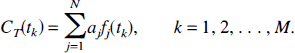
Most kinetic models used with PET tracers are based on the description of the system as a collection of well-mixed compartments with exchange of material among the compartments assumed to follow first-order kinetics. Tracer delivered to the tissue by the arterial blood exchanges with one or more compartments in the tissue, and exchange of material among the various tissue compartments can occur as well. The total concentration of tracer in the field of view of the PET camera can therefore be written as the convolution integral:

$$C_T(T)=\sum _{j=1}^n{a}_j{\int }_0^T{C}_p(t)e^{-b_j(T-t)}dt$$

[1]

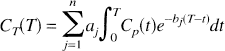
where C_p(t) denotes the arterial input function (t minutes after injection of tracer), T is the time at which the tissue activity is measured, C_T(T) is the tissue activity at time T, n is the number of compartments in the tissue, and a_j and b_j are the parameters describing exchange of tracer among the compartments, the values of which are to be estimated. ¹ The estimation problem, which is nonlinear in the parameters b_j can be converted into a linear estimation problem by predefining a large number, N, of basis functions, f_i(T) where

$$f_j(T)={\int }_0^T{C}_p(t)e^{-b_j(T-t)}dt,j=1,2,\dots ,N$$

[2]

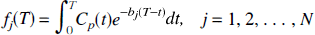
with a fixed set of values of b_j and solving for the linear coefficients a_j. The model, therefore, becomes

$$C_T(T)=\sum _{j=1}^N{a}_j{f}_j(T),$$

[3]

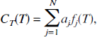
where the mathematical process now consists of estimating the N-vector

$$\underset{\_}{\mathbf{a}}=[a_1,a_2,\dots ,a_N].$$

[4]

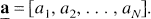
It is understood that coefficient a_j is zero if the basis function f_j(T) is not included in the model. Estimation of the coefficients a_j from equation [3], however, requires non-negativity constraints on a_j to avoid inclusion of pairs of nearly equal components with coefficients opposite in sign. For tracers that distribute into a compartment exchangeable with the plasma plus a trapped or reversibly-bound compartment, or that distribute into parallel sets of such compartments, the requirement that a_j ≥ 0 is satisfied. This includes PET tracers used for measurement of cerebral blood flow, glucose metabolism, and many receptor ligands. For these and other compartmental systems that do not contain cycles, i.e., those systems in which it is not possible for material to pass from a given compartment through two or more other compartments back to the initial compartment, the exponents b_j are real and non-negative (Hearon, 1963). The constants b_j are chosen so that they span the range of possible exponents that may be detectable in the data given the time-sampling of the tissue data and the measurement noise level.

Because continuous time measurements of the tissue concentration of tracer are unavailable, the continuous time equation [3] is replaced by its discrete time counterpart. For tissue data sampled at times t₁, t₂, …, t_M, the model equations are:

$$C_T(t_k)=\sum _{j=1}^N{a}_j{f}_j(t_k),k=1,2,\dots ,M.$$

[5]

Furthermore, measured tissue concentrations include noise, or errors in the measurement. If X(t_k) represents the measured tissue concentration at time t_k, and e_k is the error in the measurement, we have

$$X(t_k)=C_T(t_k)+{\epsilon }_k=\sum _{j=1}^N{a}_j{f}_j(t_k)+{\epsilon }_k,k=1,2,\dots ,M.$$

[6]

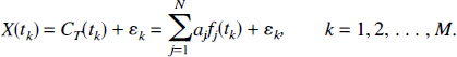
The errors are assumed to have zero mean.

Estimation of the vector $\underset{\_}{\mathbf{a}}$ from equation [6] may be carried out with either the non-negative least squares (NNLS) algorithm (Turkheimer et al., 1992) or the Simplex algorithm (Cunningham and Jones, 1993). The two solutions produced may be similar, but they are not equivalent. For a given set of weights, ² w_k, the NNLS determines the linear coefficients that minimize

$$\parallel \underset{\_}{\mathbf{r}}(a_1,a_2,\dots ,a_N){\parallel }_2^2=\sum _{k=1}^M{\left[\frac{X(t_k)-C_T(t_k)}{w_k}\right]}^2$$

[7a]

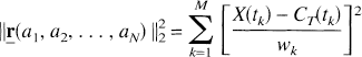
subject to a_j ≥ 0, j = 1, 2, …, N, whereas the Simplex solution is obtained by minimization of

$$\parallel \underset{\_}{\mathbf{r}}(a_1,a_2,\dots ,a_N)|=\sum _{k=1}^{M}abs\left[\frac{X(t_k)-C_T(t_k)}{w_k}\right]$$

[7b]

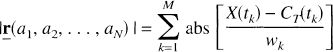
subject to the same non-negativity constraints. The symbols ‖ r ‖₂ and | r | represent the 2-norm and 1-norm of the residual vector r , respectively, and equations [7a] and [7b] are often referred to as the 2-norm, or least squares, minimization and the 1-norm, or least absolute value, minimization, respectively. Two-norm minimization leads to the maximum likelihood (ML) estimates of the coefficients when the measurement errors are independent and normally distributed whereas 1-norm minimization produces the ML estimator when errors have a double-exponential, or Laplace, distribution. The Simplex algorithm, therefore, is to be preferred when the empirical distribution of the residuals [X(t_k) – C_T(t_k)]/w_k has large tails or outlying values as it is more robust to deviations from normality of errors. For this and other issues on robust estimation the interested reader is referred to the literature (see, e.g., Tukey, 1960; Huber, 1964, 1972; Hogg, 1977). The choice between the NNLS and the Simplex algorithms is based on a priori information about noise in the data, when available, or by a posteriori examination of the residuals; statistical testing may be used to assess non-normality of residuals (see D'Agostino and Stephens, 1986), but a simple visual inspection is also recommended when sample sizes are small (Carson et al., 1983).

The result of minimization of [7a] or [7b] is an N-vector of estimated coefficients

$$\underset{\_}{\hat{\mathbf{a}}}=[{\hat{a}}_1,{\hat{a}}_2,\dots ,{\hat{a}}_N]$$

[8]

which usually contains only a few values different from zero. Results are often represented graphically by plotting the exponents b_j on the x-axis and arranging the nonzero â_j as “peaks” parallel to the y-axis; given its appearance this layout is called a “spectrum” in analogy to the spectra used in frequency analysis.

Bootstrapping in spectral analysis

A common approach for estimation of parameter uncertainties is to derive from the statistical properties of the errors in the measured data an analytical formula that describes the statistical properties of the estimated parameters. This parametric approach, however, requires a number of hypotheses concerning the distributional properties of the noise, usually that the errors at each time point be independent, normally distributed, and with a known variance. The conditions of normality and independence are not always met in PET studies (Pawlik and Thiel, 1996), and variance is known to vary between time-frames (Budinger et al., 1978).

An elegant solution to the problem of estimating parameter uncertainties in unknown noise conditions was introduced by Efron (1979), who observed that each data set is not only a sample from a population but can also be considered to be the only and best available approximation to the population itself. Therefore, we can compute numerically the variability of an estimate, not by repeatedly sampling from a theoretically well-defined population distribution, which is not available, but by resampling with replacement from the data. (For an overview of the extensive literature on bootstrap, see Efron and Tibshirani, 1993). Different ways of generating bootstrap observations are discussed below.

Bootstrapping residuals (Efron, 1979). The first, and simplest, method of generating bootstrap observations can be used if the errors on all the measurements are identically distributed with equal variance. Define the unweighted residuals as

$${\xi }_k=X(t_k)-{\hat{C}}_T(t_k),k=1,2,\dots ,M$$

[9]

where

$${\hat{C}}_T(t_k)=\sum _{j=1}^N{\hat{a}}_j{\int }_0^{t_k}{C}_p(t)e^{-b_j(t_k-t)}dt,$$

[10] Ĉ_T (t_k) are the tissue concentrations computed at time t_k with the parameters â_j estimated by the spectral analytic method, i.e., by minimization of equations [7a] or [7b]. The bootstrap procedure begins by generating a bootstrap data sample

$$\stackrel{\ast }{X}(t_k)={\hat{C}}_T(t_k)+{\stackrel{\ast }{\xi }}_k,k=1,2,\dots ,M$$

[11]

where ${\stackrel{\ast }{\xi }}_1,{\stackrel{\ast }{\xi }}_2,\dots ,{\stackrel{\ast }{\xi }}_M$ are bootstrapped residuals sampled with replacement ³ from the original residuals ${\xi }_1,{\xi }_2,\dots ,{\xi }_M$ computed from equation [9]. The spectral analysis is applied to the bootstrap data vector

$$\underset{\_}{\stackrel{\ast }{X}}=[\stackrel{\ast }{X}(t_1),\stackrel{\ast }{X}(t_2),\dots ,\stackrel{\ast }{X}(t_k)]$$

[12]

and the solution N-vector is recorded as ${\underset{\_}{\stackrel{\ast }{\mathbf{a}}}}^{(1)}$ . The bootstrap data sample generation and solution vector estimation is repeated a large number, R, of times (100 or more), and R solution vectors,

$${\underset{\_}{\stackrel{\ast }{\mathbf{a}}}}^{(i)}=[{\stackrel{\ast }{a}}_1^{(i)},{\stackrel{\ast }{a}}_2^{(i)},\dots ,{\stackrel{\ast }{a}}_N^{(i)}]i=1,2,\dots ,R,$$

[13]

are obtained. The R bootstrap solution vectors form an (R × N) bootstrap distribution matrix $\stackrel{\ast }{\mathbf{A}}$ the ith row of which contains the ith bootstrap solution vector ${\underset{\_}{\stackrel{\ast }{\mathbf{a}}}}^{(i)}$ i.e.,

$$[\stackrel{\ast }{\mathbf{A}}{]}_{ij}={\stackrel{\ast }{a}}_j^{(i)},i=1,2,\dots ,R;J=1,2,\dots ,N.$$

[14]

In addition, the N-vector $\underset{\_}{\stackrel{\ast }{\bar{\mathbf{a}}}}$ is defined as mean of all bootstrap solution vectors as

$$\underset{\_}{\stackrel{\ast }{\bar{\mathbf{a}}}}=\frac{1}{R}\sum _{i=1}^R{\underset{\_}{\stackrel{\ast }{\bar{\mathbf{a}}}}}^{(i)}$$

[15]

As stated above, this implementation of the bootstrap requires that the errors in the measurements be identically distributed with homogeneous variance. More complex resampling schemes are needed when variance of the error varies with time.

Bootstrapping pairs ( Efron, 1982 ) The generation of the bootstrap data vector $\underset{\_}{\stackrel{\ast }{X}}$ may also be done by resampling with replacement the data pairs (t_k X(t_k)). In this case a data value for every sampling time t_kk may not be included in every bootstrap data set. Because of this characteristic, the method of bootstrapping pairs is more appropriate when the independent variable is random, whereas the method of bootstrapping residuals is more suitable when the independent variable is deterministic, as it is in the case of PET data. The bootstrapping of pairs, however, can be used in the case of a deterministic dependent variable when variance in the measurements is not homogeneous (Shao, 1996).

Other resampling schemes If observations can be grouped so that measurements within each group have approximately equal variance, it is natural to resample the residuals within each group instead of resampling residuals from the entire set of observations (Hjorth, 1994). On the other hand, if one has available some estimates of the standard deviation of the residuals up to a proportionality constant, then the bootstrap residual resampling scheme can be modified as described below.

Let w₁, w₂, …, w_M be the weights proportional to the standard deviations σ₁, σ₂, …, σ_M in the measurements at sampling times t₁, t₂, …, t_M. The NNLS or the Simplex algorithm is used with the weights provided to find an estimate of the linear coefficients, i.e., a solution vector â . From the estimates of the parameters â_j, the weighted residual values, r _k , and weighted residual vector, r , are computed as

$$\begin{array}{rl}& r_k={\xi }_k/w_k,k=1,2,\dots ,M\\ & \underset{\_}{\mathbf{r}}=[r_1,r_2,\dots ,r_M]\end{array}$$

[16]

where the unweighted residual, ${\xi }_k$ is defined in equation [9]. At the next step, the bootstrap sample is constructed as

$$\stackrel{\ast }{X}(t_k)={\hat{C}}_T(t_k)+w_k{\stackrel{\ast }{r}}_k,k=1,2,\dots ,M$$

[17]

where ${\stackrel{\ast }{r}}_1,{\stackrel{\ast }{r}}_2,\dots ,{\stackrel{\ast }{r}}_M$ are bootstrapped residuals resampled with replacement from the original weighted residuals r₁, …, r₂, …, r_M and Ĉ_T(t_k) is the tissue concentration calculated from the parameter estimates â_j as in equation [10].

Note that the weight w_k corresponding to the measurement at sample time t_k is fixed; only the residuals are resampled. The bootstrap matrix $\stackrel{\ast }{\mathbf{A}}$ and the vector $\underset{\_}{\stackrel{\ast }{\bar{\mathbf{a}}}}$ , are computed after R repetitions of the resampling procedure, as in equations [13] through [15].

Application of the bootstrap procedure

Estimation of the vector of coefficients and confidence intervals Because of the non-negativity constraints imposed on the solution, the solution vector $\underset{\_}{\hat{\mathbf{a}}}=[{\hat{a}}_1,{\hat{a}}_2,\dots ,{\hat{a}}_N]$ may be a biased estimator of the true vector of coefficients a = [a₁, a₂, …, a_N]. As detailed in Appendix I, an estimate of the bias $\underset{\_}{\hat{\mathbf{B}}}$ in the estimator â can be made by subtracting â from the mean bootstrap solution vector $\underset{\_}{\stackrel{\ast }{\bar{\mathbf{a}}}}$ :

$$\underset{\_}{\hat{\mathbf{B}}}=\underset{\_}{\stackrel{\ast }{\bar{\mathbf{a}}}}-\underset{\_}{\hat{\mathbf{a}}}.$$

[18]

A new asymptotically unbiased estimator of the vector of coefficients can then be computed as

$${\underset{\_}{\mathbf{a}}}^{new}=\underset{\_}{\hat{\mathbf{a}}}-\underset{\_}{\hat{\mathbf{B}}}=\underset{\_}{\hat{\mathbf{a}}}-(\underset{\_}{\stackrel{\ast }{\bar{\mathbf{a}}}}-\underset{\_}{\hat{\mathbf{a}}}).$$

[19]

Since a ^new is corrected for bias through a numerical procedure, however, its variability will be higher than that of â , and the decrease in bias produced by use of equation [19] must be traded off against the increase in variance. When the number of bootstrap replications R is sufficiently large, then the percentiles of the distribution and confidence intervals for the solution vector â and for the estimate a ^new can be determined from the columns of the bootstrap distribution matrix $\stackrel{\ast }{\mathbf{A}}$ ; formulas for computation are given in Appendix II.

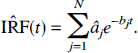
Estimation of derived parameters and their distributions Components detected with spectral analysis can be combined to obtain parameters of physiologic interest. For example, Cunningham et al. (1993) used the detected components (â_j, b_j) to obtain an estimate of the impulse response function (IRF) of the tissue as:

$$I\hat{R}F(t)=\sum _{j=1}^N{\hat{a}}_j{e}^{-b_{j}t}.$$

[20]

From equation [20] the parameters K₁, the unidirectional clearance of tracer from blood to tissue, and _Vd, the volume of distribution of the tracer in tissue relative to blood, were determined as:

$$K_1=IRF(t=0)$$

[21]

and

$$V_d={\int }_0^{\infty }IRF(t)dt.$$

[22]

The remainder of this section illustrates how spectral analysis can be used, not only to estimate the derived parameter itself, but also to estimate the statistical properties of the parameter, such as its variance and confidence intervals.

Let $\hat{\theta }$ be any parameter that depends on the coefficients a defined in equation [4], i.e.,

$$\theta =\phi (\underset{\_}{\mathbf{a}})$$

[23]

where φ is a function that describes the relationship between a and θ. In the cases described above, when θ ≡ K₁ then

$$K_1=\phi (\underset{\_}{\mathbf{a}})=\sum _{j=1}^N{a}_j$$

[24]

and when θ ≡ V_d

$$V_d=\phi (\underset{\_}{\mathbf{a}})=\sum _{j=1}^N{a}_j/b_j.$$

[25])

Let $\hat{\theta }$ be an estimate of θ determined by applying the function φ to â , i.e.,

$$\hat{\theta }=\phi (\hat{\mathbf{a}}).$$

[26]

The bootstrap distribution of $\hat{\theta }$ can be easily estimated by computing and recording, at each of the R bootstrap replications, the value

$${\stackrel{\ast }{\theta }}^{(i)}=\phi ({\underset{\_}{\stackrel{\ast }{\mathbf{a}}}}^{(i)})$$

[27]

where ${\underset{\_}{\stackrel{\ast }{\mathbf{a}}}}^{(i)}$ is the ith bootstrap estimate of the vector of coefficients (equation [13]). Let $\stackrel{\ast }{S}$ be the R-vector of bootstrap estimates of θ:

$$\stackrel{\ast }{\mathbf{S}}=[{\stackrel{\ast }{\theta }}^{(1)},{\stackrel{\ast }{\theta }}^{(2)},\dots ,{\stackrel{\ast }{\theta }}^{(R)}].$$

[28]

Then $\stackrel{\ast }{S}$ provides an estimate of the distribution $\hat{\theta }$ that can be used to establish the statistical properties of $\hat{\theta }$ . Trivially, the sample variance of the elements of $\stackrel{\ast }{S}$ can be used as an estimate of the variance of θ. $\stackrel{\ast }{S}$ can also be used for correction of any bias in the estimate $\hat{\theta }$ that results from bias in â by defining, in analogy with equation [19], the estimator:

$${\hat{\theta }}^{new}=\hat{\theta }-\{mean(\stackrel{\ast }{\mathbf{S}})-\hat{\theta }\}.$$

[29]

Finally, by ranking the set of bootstrap values from the smallest to the largest, percentiles of the distribution and confidence intervals of $\hat{\theta }$ can be obtained as detailed in Appendix II.

MATERIAL AND METHODS

Algorithm implementation

Minimization of the 2-norm (defined in equation [7a]) was performed with the NNLS algorithm described by Lawson and Hanson (1974). For minimization of the 1-norm (defined in equation [7b]), the modified Simplex algorithm of Barrodale and Young (1966) was used. Programs were written in C language⁴ for the Sun Sparkstation 20 (Sun Microsystems, Mountain View, CA, U.S.A.). Range and distribution of the exponents b_j of the basis functions were the same as those described by Turkheimer et al. (1994).

Simulation studies

To evaluate the small sample properties of the bootstrap method, simulation studies were performed as follows. Without loss of generality, the input function of the system, C_p(t), was assumed to be impulsive. With impulsive input, the convolution basis functions (equation [2]) are simple exponential functions, and the tissue concentration (equation [3]) is multiexponential. Noise conditions, time sampling, and the ratio between exponents of the functions were defined to represent a problem close to the practical limits for identification of separate exponential functions, as reported in the literature (Yeramian and Claviere, 1987). The biexponential test function was:

$$C_T(t)=exp(-0.2t)+exp(-0.4t).$$

[30]

The data

$$X(t)=C_T(t)+\epsilon (t)$$

[31]

were sampled at 15 time points (t = 0,0.1,0.3,0.5, 0.7, 1, 1.5, 3, 5, 7.5, 10, 15, 20, 25, 35 minutes), and ε(t_k) was randomly generated, independent and normally distributed at each time point, with 5% coefficient of variation. One hundred basis functions were given by

$$f_j(T)=exp(-b_{j}T),j=1,2,\dots ,100,$$

[32]

and the exponents b_j were logarithmically distributed (Turkheimer et al., 1994) between 0.01 min⁻¹ and 10 min⁻¹. To simulate realistic conditions the standard deviations in the measurements were assumed to be unknown but to have a constant coefficient of variation. The data points themselves, X(t_k), were used as the weights w_k.

In each simulation 1,000 different data sets were generated. For each data set h, the NNLS algorithm was used to estimate the coefficients, â _(h) (h = 1,2, …, 1000) (equation [8]). Then 1,000 bootstraps were used to compute the mean bootstrap solution vector for data set $h,{\underset{\_}{\stackrel{\ast }{\bar{\mathbf{a}}}}}_{(h)}$ (equation [15]) and the bias-corrected coefficients, a ^new_(h) (equation [19]). When all 1000 simulations were completed, the mean of the estimated coefficients,

$$\underset{\_}{\bar{\mathbf{a}}}=\frac{1}{1000}\sum _{h=1}^{1000}{\underset{\_}{\hat{\mathbf{a}}}}_{(h)},$$

[33]

the mean of the mean bootstrap solution vectors,

$$\underset{\_}{\stackrel{\ast }{\bar{\mathbf{a}}}}=\frac{1}{1000}\sum _{h=1}^{1000}{\underset{\_}{\stackrel{\ast }{\bar{\mathbf{a}}}}}_{(h)},$$

[34]

and the mean of the bias-corrected coefficients,

$${\underset{\_}{\bar{\mathbf{a}}}}^{new}=\frac{1}{1000}\sum _{h=1}^{1000}{\underset{\_}{\mathbf{a}}}_{(h)}^{new},$$

[35]

were computed.

For each simulated data set, the derived parameter ${\hat{K}}_1$ (equation [24]), its bias-corrected estimate ${\hat{K}}_1^{new}$ (equation [29]), the bootstrap estimate of the variances of ${\hat{K}}_1$ and ${\hat{K}}_1^{new}$ and the two-sided 90% confidence intervals were recorded.

[¹⁸F]Fluorodeoxyglucose studies

The method was applied to the reexamination of [¹⁸F]fluorodeoxyglucose ([¹⁸F]FDG) PET scans of a normal male subject whose study was previously described (Lucignani et al., 1993). The data set consisted of 31 scans acquired according to the following schedule: 5 scans of 1 minute each, 5 scans of 2 minutes each, and 21 scans of 5 minutes each for a total scanning time of 120 minutes. The arterial plasma input function, C_p(t), was measured by collecting blood samples from the radial artery after a pulse of approximately 8 mCi of [¹⁸F]FDG was injected, rapidly centrifuging the samples, and assaying the plasma ¹⁸F concentrations. Anatomic ROIs were drawn on the images and the time course of total radioactivity in each ROI obtained. In addition, the time course of the whole-brain radioactivity was determined as the weighted average of the radioactivity in all image planes. All data were corrected for radioactive decay.

The basis functions consisted of 100 exponential functions convolved with the measured arterial plasma input function, C_p(t). The range of the exponents was from b_j = 3 min⁻¹ to b_j = 0.0028 min⁻¹. Two additional components were added, the integral of the input function (equivalent to a component with b_j = 0) and the input function itself (equivalent to a component with b_j = ∞), the latter to account for the blood pool in the tissue. The minimization procedure was weighted with estimates of the standard deviation in the tissue measurements, computed as described in Budinger et al. (1978). For each ROI, the bootstrap distribution of the coefficients, the 90th percentiles of the distribution, and the bias-corrected coefficients were estimated with 1,000 bootstraps.

In the [¹⁸F]FDG studies, the coefficient of the integral of the arterial plasma concentration, which we denote by a₀, is proportional to the rate of glucose utilization in the tissue (Turkheimer et al., 1994). However, noise in the data can lead to a shifting of the detected components away from the peak in the spectrum at b_j = 0 and a subsequent bias in estimating the rate of glucose utilization. One method proposed to compensate for this effect was to add all coefficients of components whose exponents fell below a certain cutoff frequency β_cutoff (Cunningham and Jones, 1993). In each ROI examined in the current study, this parameter K, the rate constant for unidirectional trapping of tracer, was estimated from the bias-corrected coefficients as

$$\hat{K}=\sum _j\{a_j^{new}foralljwith{b}_j<{\beta }_{cutoff}\}.$$

[36]

A cutoff threshold of 1/120 minute was used. In addition, the probability distribution and 90% confidence intervals for $\hat{K}$ were determined.

H215O studies

As a second example, the method was used for the analysis of brain time-activity curves during an infusion of [¹⁵O]-labeled water (H₂¹⁵O) to measure cerebral blood flow. The H₂¹⁵O was infused into an antecubital vein of a normal male subject by an infusion pump (Model 44, Harvard Apparatus, South Natick, MA, U.S.A.) programmed to produce a rapid increase in brain tissue concentration of H₂¹⁵O and keep it elevated for 3 minutes, at which time the infusion was terminated. Measurement of the H₂¹⁵O concentration in arterial blood was initiated just before the infusion of the H₂¹⁵O and continued until the end of scanning by continuously withdrawing blood from a radial arterial catheter past a NaI detector. The dead space of the tubing leading from the artery to the detector, as well as the pump withdrawal rate were fixed, and the dispersion of the arterial curve through this sampling system was well characterized (Jaggi et al., 1997). Brain scanning was initiated concurrently with the start of infusion with a UGM180 scanner (UGM Medical Systems, Philadelphia, PA, U.S.A.) and consisted of six 5-second scans, six 10-second scans, and six 20-second scans. Regions of interest were placed on a number of gray matter structures. Before the application of the spectral analysis bootstrap method, the input function was corrected for estimated delay.

One hundred basis functions consisting of exponential functions convolved with the measured arterial whole blood input function were used. Exponents ranged from b_j = 0.1 min⁻¹ to b_j = 10 min⁻¹, and the input function and its integral were also included. The minimization procedure was unweighted, and, as with the FDG data analysis, 1,000 bootstraps were used to estimate the distribution of the coefficients, the 90th percentiles, and the bias-corrected coefficients.

RESULTS

Simulation studies

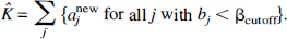
Small differences between the mean of the coefficients computed for each of the simulations, $\underset{\_}{\bar{\mathbf{a}}}$ , and the mean of the bootstrap estimates, $\underset{\_}{\stackrel{\ast }{\bar{\mathbf{a}}}}$ , were detected when noise was normally distributed and the NNLS algorithm was used (Fig. 1A). Use of the bootstrap bias correction procedures yielded estimates ${\underset{\_}{\bar{\mathbf{a}}}}^{new}$ that were in closer agreement to the true mean values (Fig. 1B). Results did not change when the number of bootstrap samples was increased to 5,000, when the Simplex algorithm was used, or when the algorithms were used with more heavy tailed error distributions (data not shown).

FIG. 1.

Results of simulation to examine properties of the bootstrap estimator. The biexponential function f(t) = a₁ exp (−b₁ t) + a₂ exp (−b₂ f), with b₁ = 0.4 min⁻¹, b₂ = 0.2 min⁻¹, a₁ = a₂ = 1, was sampled at times between 0 and 35 minutes. One thousand sample sets of 5% normally distributed noise were generated and added to the sample data; for each noisy data set a spectrum, a bootstrap spectrum, and a bias-corrected bootstrap spectrum were calculated. (A) Triangles show the mean of the computed spectra, $\underset{\_}{\bar{\mathbf{a}}}$ , and circles the mean of the bootstrap spectra, $\underset{\_}{\stackrel{\ast }{\bar{\mathbf{a}}}}$ . Exponents b_j are on the x-axis, and the corresponding linear coefficients a_j are displayed as peaks in the y-direction. (B) Mean of the bias-corrected bootstrap spectra a ^new (circles) is compared with the mean of the simulation spectra (triangles). On average, the bias-corrected bootstrap spectrum provides a more accurate estimation of the mean spectrum that would be obtained if repeated noisy sample data sets were available than does the bootstrap spectrum without bias correction.

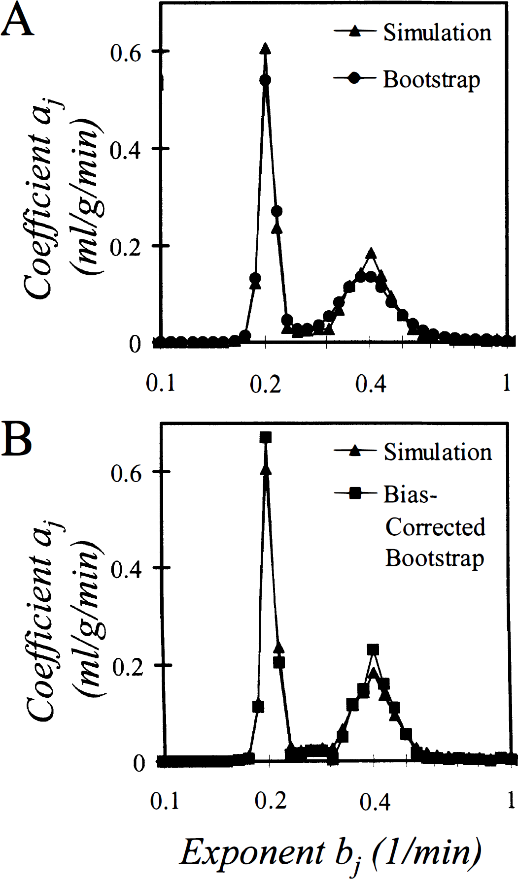
A schema illustrating the bias-correction procedure for the derived parameter K₁ is given in Fig. 2. Simulation results for the parameter K₁ confirmed the theoretically expected tradeoff between decreasing bias and increasing variance in the estimate. The true value of K₁ in these simulations was 2.0, and the mean value of the estimate ${\hat{K}}_1$ over all simulations was found to be 2.031. The bias-corrected estimate ${\hat{K}}_1^{new}$ reduced the bias by 36% (mean( ${\hat{K}}_1^{new}$ ) = 2.020) at the expense of a 7% increase in variance (var( ${\hat{K}}_1^{new}$ ) = 0.0049; var( ${\hat{K}}_1$ ) = 0.0046). The mean of all the bootstrap estimates of the variance of ${\hat{K}}_1$ was 0.0052, a 13% overestimation of the variance determined in all the simulations. The two-sided 90% confidence interval of ${\hat{K}}_1$ (determined over all simulations) was [1.932, 2.156]; the mean of the bootstrap-estimated confidence intervals was [1.946, 2.125]. This shows that the bootstrap can be used to obtain useful numerical approximations of parameter variance and confidence intervals.

FIG. 2.

Schema illustrating the bias-correction procedure for a derived parameter. Values of the derived parameter K₁ are shown along the x-axis, and the probability density function for the parameter, p(K₁), is given on the y-axis. The biexponential function f(t) = 1 exp (−0.4 t) + 1 exp (−0.2 t) was sampled at times between 0 and 35 min as in Fig. 1. Fifteen percent normally distributed noise was generated and added to the sample data, the estimated coefficients $\underset{\_}{\hat{\mathbf{a}}}$ were determined by the non-negative least squares algorithm, and the derived parameter K₁ was estimated by use of equation [24]. The estimated value ${\hat{K}}_1$ is shown as the vertical dotted line in the center of the figure. The bootstrap distribution of the parameter (unbroken curve) and the mean of the distribution ( ${\bar{K}}_1$ unbroken vertical line) were comRuted with 1,000 bootstraps. Note that the estimated parameter, ${\hat{K}}_1$ and the mean of the bootstrap distribulion, ${\bar{K}}_1$ are not equal; their difference is the estimated bias in ${\hat{K}}_1$ . The estimated bias was then used to form the bias-corrected estimate ${\hat{K}}_1^{new}$ (equation [29]; center vertical dashed line) and its bias-corrected distribution (equation [A.18]; dashed curve). From the bias-corrected distribution of the parameter, other statistics conceming the parameter estimate can be computed, e.g., the 90% confidence interval for ${\hat{K}}_1^{new}$ (dashed vertical lines at left and right of figure).

Computation time for evaluation of a ^new for each sample was approximately 40 seconds for the Simplex algorithm and 45 seconds with NNLS.

[¹⁸F]Fluorodeoxyglucose studies

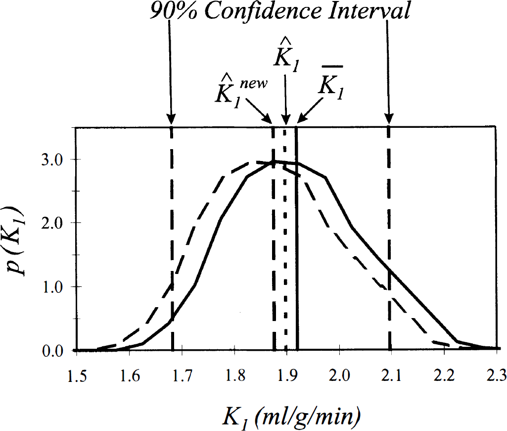
Results of the analysis of FDG data are displayed for the whole brain (Fig. 3A), a small white matter region (Fig. 3B) and a large ROI drawn over the visual cortex (Fig. 3C). The computed spectra shown in the left panels are consistent with previously computed spectra of FDG tissue data (Cunningham and Jones, 1993; Turkheimer et al., 1994). The peak on the far left, labeled a₀, corresponds to the coefficient of the integral of the arterial plasma input function and indicates irreversible trapping of the tracer in the tissue, i.e., b_j = O. The components detected at b_j = 0.06 min⁻¹ and b_j ≅ 0.6 min⁻¹ have been associated with exchangeable tissue compartments in white and gray matter, respectively (Turkheimer et al., 1994). Because of the partial volume effect of the scanner, heterogeneity was detected in all regions, even those in which the ROI was placed over an area that was predominantly white matter (Fig. 3B), or predominantly gray matter, such as the visual cortex (Fig. 3C). The fourth peak, detected at b_j 2.5 min⁻¹, is consistent with a rapid equilibration of the tracer in the tissue and has been associated to delay and dispersion of the measured input function (Cunningham and Jones, 1993).

FIG. 3.

Results of spectral analysis with bootstrap resampling applied to brain tissue-activity curves after intravenous injection of [¹⁸F]fluorodeoxyglucose into a human subject. Regions shown are whole brain (A), a small white matter region (B), and the visual cortex (C). In the left panels the bootstrap spectra (heavy line) are compared to the spectrum computed on the raw data (thin line); right panels show the 90% confidence intervals (thin line) and the bias-corrected bootstrap spectra (heavy line). The coefficient shown on the far left, labeled a₀, is the coefficient of the integral of the plasma curve; it is proportional to the rate of glucose utilization in the tissue. Note that in the whole brain and visual cortex the estimate of a₀ is very stable; its initial estimate and its bias-corrected estimate are in close agreement. In contrast, in the higher noise white matter region, there is high uncertainty in the estimate of a₀ as evidenced by the lack of agreement between the initial estimate, the bootstrap estimate, and the bias-corrected bootstrap estimate. Additionally, observe that the noise in the white matter region has led to spreading of the peak around a₀ The blood volume component is not shown.

The bootstrap spectra, shown in the heavy lines in the left panels, allow one to make inferences concerning the uncertainty of the detected peaks. The first and most expected is the increased width of the peaks in the relatively higher noise region, i.e., the white matter region (Fig. 3B), compared to the lower noise data sampled in the whole brain (Fig. 3A) or large gray matter region (Fig. 3C). Additionally, the bootstrap spectra indicate a greater variability in the peak associated with the gray matter exchangeable compartment (b_j ≅ 0.6 min⁻¹) than in the more slowly exchanging compartment (b_j = 0.06 min⁻¹); this may be caused by a combination of the higher noise level in the first minutes of scanning, which largely determine the faster component, and the greater heterogeneity of gray matter.

In the right panels are shown the 90th percentiles of the distribution of the coefficients and the bias-corrected spectra. The greater uncertainties in the coefficients in the higher noise white matter region are seen as broader “shoulders” on the peaks in the 90th percentile of the distribution. In particular, in the white matter region the coefficient a₀ of the integrated component at b_j = 0 min⁻¹ was computed to be 0.020 mL·g⁻¹·min⁻¹, but its 90th percentile was found to be 0.032 mL·g⁻¹·min⁻¹, indicating a large degree of uncertainty in the estimate. By contrast, in low to medium noise conditions (Figs. 3A and C) the bias-corrected coefficient a₀ and its 90th percentile are within 1% of the initially computed value.

Distributions for the estimated rate constant for unidirectional trapping of tracer are shown in Fig. 4. In the whole brain and the visual cortex there is an extremely small spread of the parameter estimate about its mean value. The mean value and 90% confidence interval of the estimate $\hat{K}$ in whole brain were 0.03180 mL·g⁻¹·min⁻¹ and [0.03171, 0.03187], respectively; corresponding values in the visual cortex were 0.03494 mL·g⁻¹·min⁻¹ and [0.03483, 0.03507]. In both regions, 90% of the distribution fell less than 1% distant from the mean. The white matter region, which has fewer counts and thus higher noise levels, exhibits a much more broadly spread distribution: the mean and 90% confidence interval were 0.0206 mL·g⁻¹·min⁻¹ and [0.0178, 0.0230], respectively. In this region, the 90% confidence interval falls only within 14% of the mean.

FIG. 4.

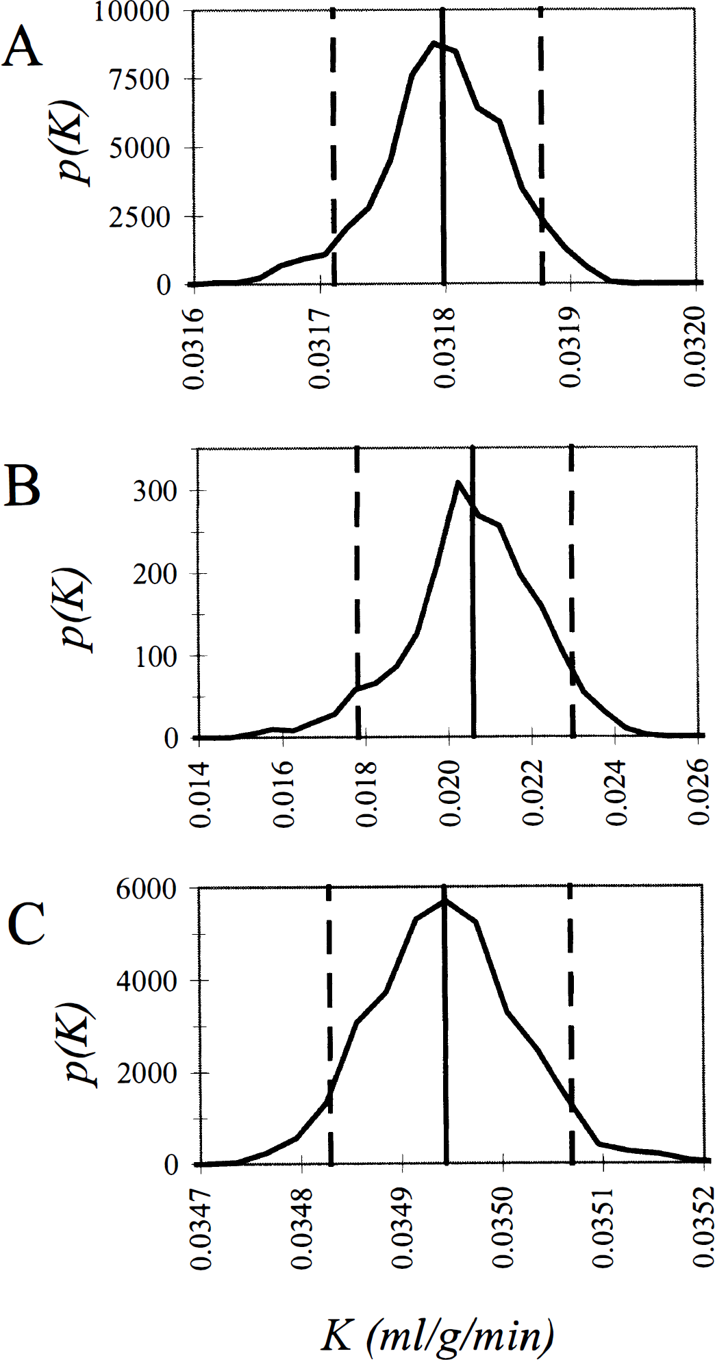
Probability density functions for the estimated rate constant for unidirectional trapping of tracer, K after intravenous injection of [¹⁸F]fluorodeoxyglucose into a human subject. In the presence of noise in the data, the parameter K leads to a more accurate determination of glucose utilization than the coefficient a₀ (see Fig. 3). K is computed as the sum of those coefficients a_j for which the corresponding exponents b_j fall below a cutoff threshold (see text). Shown are the bias-corrected estimate of K (vertical unbroken line), its probability distribution function (unbroken curve), and its 90% confidence interval (vertical dashed lines) for the whole brain (A), a small white matter region (B), and the visual cortex (C). In the whole brain and the visual cortex there is an extremely small spread of the parameter estimate about its mean value. The white matter region, which has fewer counts and thus higher noise levels, exhibits a broadly spread distribution.

H215O studies

Figure 5 shows the computed and bootstrap spectra (left panel) and the bias-corrected and 90th percentile spectra (right panel) resulting from the analysis of the time course of tissue radioactivity in the cerebellum during infusion of H₂¹⁵O. Whereas the computed spectrum is consistent with preceding analyses that have detected two peaks (Cunningham and Jones, 1993), new information concerning the variability of the two components is provided by the bootstrap spectrum. The first peak (b_j = 0.7 min⁻¹) represents relatively rapid exchange of tracer between blood and tissue; it probably corresponds to blood flow in the gray matter tissue. The uncertainty on the exponent b_j is rather high; this is consistent with the observation that spectral analysis of H₂¹⁵O time activity curves does not lead to precise estimates of cerebral blood flow values (Cunningham et al., 1993).

FIG. 5.

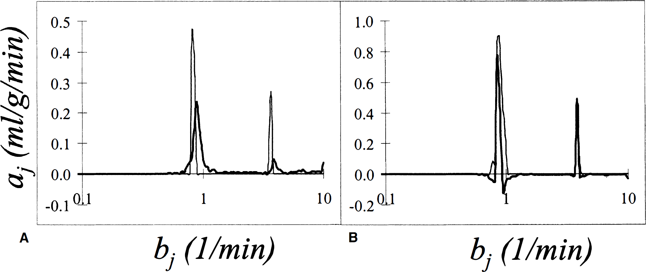
Results of spectral analysis with bootstrap resampling applied to brain tissue activity curves measured during infusion of ¹⁵O-labeled water into a human subject. Data are for a region of interest placed over the cerebellum. In (A) the computed spectrum (thin line) and bootstrap spectrum (heavy line) are shown; (B) illustrates the 90% confidence interval (thin line) and the bias-corrected bootstrap spectrum (heavy line). The left peak is associated with blood flow in the gray matter and the right peak with dispersion of the input function. Even though the region is known to be heterogeneous because of the limited spatial resolution of the PET camera, no peak associated with white matter flow was detected. A blood volume coefficient was detected but is not shown on the graph.

It is interesting to observe the lack of a peak that can be associated with white matter flow even though white matter is known to be present in all ROI because of the limited spatial resolution. The magnitude of the coefficient of the white matter flow component is expected to be small and is probably not detectable at the given noise levels; in addition the length of the sampling schedule may be inadequate for the detection of the much slower white matter component.

The very fast peak (b_j ≅ 4 min⁻¹), related to dispersion and delay in the input function, is also determined with a large degree of uncertainty. The 90th percentile of its coefficient, 0.47 mL·g⁻¹·min⁻¹, is almost twice its computed value of 0.27 mL·g·min⁻¹. Although its value cannot be precisely estimated by the spectral analysis technique, the presence of the very fast peak must be taken into account for any further modeling as previously discussed (Cunningham et al., 1993).

DISCUSSION

This report proposes a method to estimate the statistical distributional properties of the components determined by spectral analysis and of parameters derived from those components when the method is applied to a single data set. The method uses the bootstrap technique to estimate the mean effect of noise on the computed spectrum, to estimate bias in the bootstrap spectrum, and to correct for that bias. The bias-corrected bootstrap spectrum was shown to be a good estimator of the average spectrum that would have been obtained if repeated samples of the measured data set were available. Assumptions concerning the distributional properties of noise in the data are minimal, and specific implementations of the bootstrap procedure have been considered to handle the case of inhomogeneity of variance in the measured data.

The application of the method to two sets of PET dynamic data was also presented to illustrate the main property of the bootstrap estimator, i.e., it provides an assessment of the uncertainty of the computed peaks, and gives a preliminary picture for the subsequent modeling or parameter estimation. The proposed method does not eliminate the need to use biochemical or physiologic information obtained from other sources to interpret the dynamics of the system.

It is also worth noting that application of spectral analysis to the data in this report has relied on the assumption that the kinetic behavior of the system can be described by a non-negative linear combination of the chosen basis functions. Non-negativity of the linear coefficients is an essential requirement of this approach; other analysis methods must be applied if the system does not satisfy this constraint. If the system requires functions other than convolution integrals, the method can be applied only if another set of basis functions, valid for the system under study, is defined.

Finally, because the bootstrap procedure is computer intensive, its use may be limited in the case of very large data sets as in the voxel-by-voxel analysis of PET volumes.