
Abstract
A novel data collection strategy was examined for positron emission tomography activation studies. After an injection of H215O, data were collected in multiple 10-second frames and analyzed with a blocked analysis of variance design in which blocking was performed across frames. An estimate of residual error based on a larger number of statistically independent measurements was hence obtained and the statistical significance of detected differences increased. The feasibility of the suggested scheme was demonstrated on phantom data, where higher significance was achieved when dividing the same data into more frames. The method was further used for single-subject analysis of data from eight human subjects participating in a study on visceral sensation. The results show agreement with the group-based analysis and indicate that it is possible to detect areas with changes of 10 mL/(min · 100 mL) or more in single subjects. The residuals from the statistical analysis were analyzed and did not indicate any violations of the assumptions of statistical independence between frames, normal distribution of errors, and homoscedasticity across blocks. The specificity was worse than the theoretically expected 0.05, but this may have resulted from lack of complete control over the experimental situation rather than the statistical method per se.
Activation studies with positron emission tomography (PET) have long been an outstanding tool in the study of the functional organization of the human brain. Studies usually are performed measuring blood flow (Fox and Raichle, 1984), which is an indicator of neural activity, but may equally well be performed using a marker of a more specific function (Carson et al., 1995; Fischer et al., 1995; Morris et al., 1995). Methods have been developed (Worsley et al., 1992; Friston et al., 1995) to evaluate a statistic at each location in the brain and to assess the significance of these values (Worsley et al., 1992; Friston et al., 1994). These methods are based on traditional statistical tools such as t tests (Worsley et al., 1992) or analysis of variance/covariance (ANOVA/ANCOVA) (Friston et al., 1995), but the assessment of significance is hampered by special problems from the simultaneous measurement in numerous partially interdependent locations. This imposes almost forbiddingly high demands, where a z score typically needs to be in the range of 4.4 to 4.6 to be significant at the 0.05 level.
The most commonly used statistical tool, statistical parametric mapping (Friston et al., 1995), estimates a t value, from a linear combination of effect parameters estimated through an ANOVA/ANCOVA, that is subsequently converted to a z score through a probability-preserving transform (Friston et al., 1991). Hence, the resulting z score, and the validity of the transformation (Worsley et al., 1996), is strongly dependent on the degrees of freedom available for the estimation of the residual error. Experiments should be designed such that df ≥ 30 (Friston et al., 1995), and that if df < 8, it is effectively impossible to demonstrate significant activation, regardless of its magnitude (Andersson et al., 1995a).
However, when considering robust activations such as visual or somatosensory input, often it is obvious from studying a subtraction image from a single subject that (1) an activation has occurred, and (2) where it is located. This mismatch between what is obvious to the eye and still impossible to demonstrate with existing statistical methods leads to the notion that data currently are used in a suboptimal way.
CBF activation studies usually consist of several injections of 15O-H2O, after which data are collected for a 40- to 100-second period after injection. The summed data from each injection then are contrasted to reveal areas with elevated perfusion. This report explores an alternative strategy in which data after an injection are divided into several statistically independent frames, each representing an independent realization of the signal of interest. These frames are subsequently analyzed using a blocked ANOVA design, where blocking is performed across frames.
The validity and usefulness of the strategy is demonstrated on a phantom study and in human material using visceral sensation as stimulation paradigm.
MATERIALS AND METHODS
Rationale
The analysis of a PET activation study consists of evaluating a statistical entity, typically a t value or a z score, and subsequently testing the probability that the value has occurred by chance only. The magnitude of the statistical entity depends strongly on the signal-to-noise ratio of the scans, whereas the probability associated with a given value is governed by the number of statistically independent measurements used for the assessment of the residual variance. The signal-to-noise ratio may be improved through scanner design (Cherry et al., 1991), dose fractionation (Cherry et al., 1993a), and manipulation of stimulus (Volkow et al., 1991; Cherry et al., 1995) or data handling (Andersson and Schneider, 1997), whereas the number of independent measurements is increased by raising the total number of injections. Typically, 6 to 12 injections are performed in each of four to eight subjects, resulting in degrees of freedom in the range of 15 to 80.
Because of the many spatially separated independent measurements (typically several hundred), the z score significance threshold yielding an experiment-wise type 1 error of 0.05 is high, typically above 4. This means that the part of the t distribution of interest for PET activation studies is far out into the tails, a region where the difference between 5 and 20 df may make all the difference. Notice, for example, that the t value corresponding to P = 0.0001 (roughly corresponding to an experiment-wise error of 0.05) is 4.53 for df = 20, but 9.68 for df = 5. Although less easily demonstrated, the same type of arguments also hold when assessing significance through spatial extent (Friston et al., 1994). For practical purposes, a lower limit of df = 30 has been recommended (Friston et al., 1995), although lower values have to be accepted for single-subject studies (Friston et al., 1995). The feasible number of injections in a single-subject range from 6 for a two-dimensional scanner to 24 for a three-dimensional system (Cherry et al., 1993a), leaving 4 to 22 df for a two-state design.
However, the number of injections that are possible to perform in a single-subject study is limited not only by the absorbed dose to the subject, but also by practical, economic, and physiologic factors. Even if it is possible, from an absorbed dose perspective, to perform up to 24 injections in a single subject, these studies put high demands on the subjects, block the scanner and cyclotron for the major part of a day, and may produce inconsistencies resulting from learning and adaptation effects.
Hence, an ideal method would produce an adequate number of statistically independent realizations in as short a time as possible. We suggest that this may be achieved by collecting data in multiple frames (exposures) after an injection of H215O. Frame 1 for injection 1 may then be subtracted from frame 1 for injection 2, and so on, in a paired manner, yielding degrees of freedom for the resulting t statistic equal to the number of frames minus one. When extending the protocol to more than two experimental states, the same concept may be generalized to a blocked ANOVA where blocking is performed across frames. The reason for performing the blocking is that the difference in activity concentration between low- and high-flow areas decreases with the time after injection (Herscovitch et al., 1983). Therefore if blocking were not performed, the residual variance of values corrected for global activity would be augmented and hence the t values diminished.
Notice that the suggested strategy does not increase signal-to-noise ratio and that the noise equivalent counts (Strother et al., 1990) remain the same. Hence the average t value does not change; what changes is the distribution of values and consequently the probability that is attributed to a given t value.
Theory
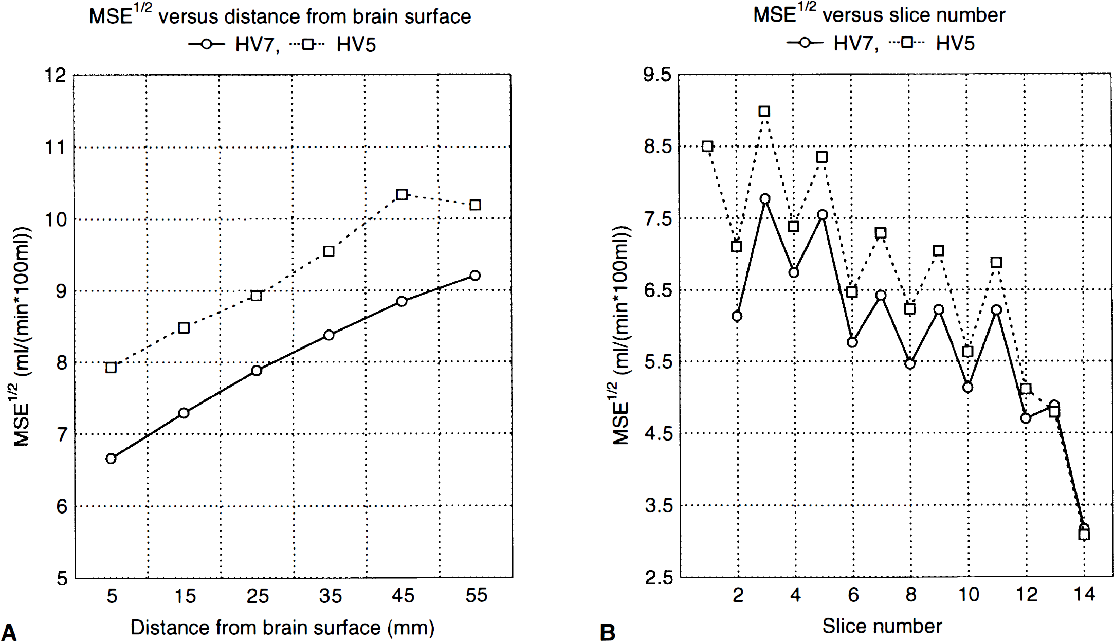
The statistical model, describing the behavior of a specific voxel, used in the current study may be described as
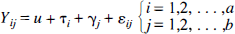
where τ denotes effects caused by physiologic state, and γ is attributable to a specific frame, or in matrix terms

where
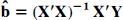
where ̂
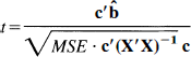
with (ab – a – b + 1) degrees of freedom, where
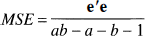
and where
There is in principle nothing to prevent the concept of multiple frames as statistically independent realizations to be extended to multisubject studies. The statistical model described in equation 1 then is extended to include an additional blocking direction for subjects
Furthermore, the inclusion of additional terms such as task-by-frame or task-by-subject interactions into equation 6 is facilitated by the additional degrees of freedom offered by the division of data into frames.
Implementation
The statistical methods briefly outlined in equations 1 through 6 have been implemented as part of a software package for analysis of PET activation studies. The software is capable of generating and handling design matrices with up to eight levels of a single-factor, one continuous effect parameter, blocking in up to four orthogonal directions, each with an unlimited number of levels, and one continuous confounding variable (covariate). Any number of contrast vectors may be entered, yielding t maps that are subsequently transformed to z score maps (Friston et al., 1991). The z score maps are searched for local extremes, and contiguous clusters of voxels with z scores above a user-defined threshold are identified. The omnibus significance of each contrast (Worsley et al., 1995), and the significance of each peak and cluster (Friston et al 1994) are estimated according to previously published methods.
The software is able to export the raw pixel values, pixel values normalized for global flow and, optionally, also corrected for other confounding effects (blocks). This may be done for any number of user-specified voxels and automatically for all local maxima/minima in clusters significant at a user-specified level. Data are exported in a format suitable for import into a commercial statistical package (Statistica, StatSoft, Tulsa, OK, U.S.A.), which may subsequently be used to test the accuracy of the calculations and to perform additional tests and calculations.
The implementation is performed in C on a VMS system and currently is capable of handling only images generated by the GEMS PC2048 or PC4096 systems (General Electric Medical Systems, Milwaukee, WI, U.S.A.).
Experiments
Scanners. Human studies were performed on a Scanditronix/GEMS PC2048-15B scanner (Holte et al., 1989) and the phantom study on a Scanditronix/GEMS PC4096-15WB scanner (Kops et al., 1990). Both scanners produce 15 contiguous 6.5 mm—thick slices and have a 6-mm axial and transaxial resolution.
Phantom study. A cylindrical phantom with an outer and inner diameter of 205 and 195 mm, respectively, containing five thin-walled glass spheres with inner-diameters of 14, 21, 25.5, 33, and 39 mm, respectively, was scanned under “baseline” and “activated” conditions. The phantom was filled with water, and two transmission scans was performed; one with air and one with water in the spheres. The phantom was removed from the scanner and filled, as were the spheres, with a concentration of 62.8 kBq/mL of 18F-fluoride. After repositioning of the phantom, 15 consecutive scans were performed, each time collecting a total of 5 · 106 events. Finally, the spheres were refilled with an activity concentration that was 7.6% higher than that in the surrounding media, and another 60 scans with 5 · 106 counts each were performed.
Human Study. Eight healthy volunteers (HV), seven men and one woman, aged 24 to 47 years, were included in the study. Each subject first underwent a T1-weighted and a T1-inversion recovery magnetic resonance (MR) imaging scan on a Philips Gyroscan ACS 1.5T (Phillips Medical Systems, Eindhoven, The Netherlands). Before PET scanning, they were asked to swallow an inflatable balloon catheter such that the balloon was located in the smooth muscle region of the esophagus. The sensation and pain threshold of each subject was tested by periodic (0.5-Hz) inflations and deflations, with gradually larger inflation volume until two different volumes were found that generated (1) definite but not painful, and (2) painful sensations. The subject was blindfolded, placed in the scanner such that the 10-cm axial field of view covered approximately the area from the vertex of the brain down to the level of commisures minus 20 mm, and the head was immobilized using a fast-hardening foam in a specially designed head holder. A transmission scan, collecting approximately 50 to 150 counts per projection member through the central parts of the brain, was performed. Lights were dimmed, and only the person performing the injection and the person administering the stimulation were allowed to remain in the scanner room. Stimulation consisted of cyclic (0.5-Hz) inflations and deflations of the balloon, where the amplitude was set either to sensory threshold (SENS) or to painful threshold (PAIN). Stimulation started 10 seconds before injection of 800 to 1000 MBq of H215O and continued until the activity levels in the brain, as assessed by the scanner count rate, had peaked (Volkow et al., 1991; Cherry et al., 1995). Each subject had two scans in each of three states: no stimulation (BASE), sensory stimulation (SENS), and painful stimulation (PAIN). The sequence of the scans were alternated between the subjects to balance out any time effects. The scanner was started at the time of the injection, and data were collected in 20 frames, each lasting for 10 seconds.
Data were summed from the time of bolus arrival to the brain and 100 seconds forward, creating a summation file. The summation file and the individual frames were reconstructed using the transmission scan for attenuation correction, correcting for scattered radiation (Bergström et al., 1983) and prefiltering the projections with a 15-mm Hanning filter.
Movements between scans were assessed from the summation images (Andersson, 1995), and corrections were made accordingly if exceeding 0.5 mm or 0.5 degrees in any direction. In those cases, the individual frames were reoriented using the same transformation matrix as for their appurtenant summation file. The individual MR imaging scans were reoriented to match the orientation of a PET summation image averaged over all states for each subject (Andersson et al., 1995b). Intersubject registration was performed manually on the MR images (Greitz et al., 1991), and the resulting transformation also was applied to the PET summation images, mapping all subjects into the “Greitz-space.”
Analysis
Validation was performed by comparing the results obtained with the suggested strategy to the known answer, in the case of the phantom data, and to the results obtained from a group-based analysis of the human material. Furthermore, an extensive analysis of residuals was undertaken to assess any violations of the underlying assumptions of the statistical model.
Phantom study. The first 12 “baseline” and the first 48 “activated” phantom data sets were used for the analysis. Data were divided so as to mimic a study with five states (one baseline and four activated) and four contrasts (–1 1 0 0 0, −1 0 1 0 0, −1 0 0 1 0, −1 0 0 0 1) were used to yield four estimates of significance of activation. First, the data sets were summed six and six together, thereby representing a study with two subjects, but with good signal-to-noise ratio for each subject. Second, data were summed four and four together, hence mimicking a study in three subjects. In this manner, data were summed to represent a study in 2, 3, 4, 6, and 12 subjects. Data subsequently were analyzed with a blocked ANOVA, and significance of each sphere was assessed both using the peak value and the size of connected clusters with z score larger than 2.6 (Friston et al., 1994). Notice that exactly the same data were used for each analysis, and that the only difference was in the way data were divided into frames.
Human Study. The stereotactically normalized summation files from all subjects were analyzed with a randomized block ANCOVA (Friston et al., 1990), looking specifically at three contrasts: (–1 1 0) depicting visceral sensation, (–1 0 1) depicting painful visceral sensation, and (0 −1 1) depicting pain-specific responses. The significance of detected clusters were assessed both using spatial extent and peak value (Friston et al., 1994), and a cluster yielding P < 0.05 according to at least one of these criteria was deemed significant. The anatomical identification of activated areas was achieved with guidance from the computerized brain atlas data base (Thurfjell et al.; 1995) and from the coregistered MR data averaged over subjects.
The individual frames for each scan were screened to determine when the bolus reached the brain. Frames 2 to 11, after arrival of bolus, were included in the analysis, which consisted of global scaling followed by a block ANOVA. Ten blocks (frames) and six factor levels (BASE1, BASE2, SENS1, SENS2, PAIN1, PAIN2) were used, and the contrasts (−1 −1 1 1 0 0), (−1 −1 0 0 1 1), and (0 0 −1 −11 1) were used for a direct comparison with the group-based analysis. An additional NULL contrast (−1 1 1 −1 −1 1) was included to yield an appreciation of the specificity. The significance of activated areas was estimated as described earlier, and significant increases for the three first contrasts, and increases and decreases for the NULL contrast, were reported. Notice that the statistical tests were two-tailed in both cases and that the limitation to increases was done to facilitate interpretation and to limit the amount of data. Anatomical identification again was aided by the computerized brain atlas and by each subject's coregistered MR scan.
Maps of the square root of the mean square error (MSE1/2) were analyzed to determine whether a local estimate of variance was necessary. Regions of interest (ROI) covering the entire brain were drawn in all slices to assess the variability between slices. Furthermore, concentric 1 cm—wide ROI enclosing the brain surface was used to estimate the dependence of depth of emission.
The raw pixel values for local maxima in all activated and false-positive clusters and several randomly chosen voxels were exported to a commercial statistical package (Statistica, StatSoft, OK, U.S.A.). Data were reanalyzed with the same statistical model; the residuals were examined to screen for violations of assumptions, such as normal-distributed errors and statistical independence between frames. The analysis consisted mainly of visual examinations of plots of residuals versus dependent and independent factors, probability—probability plots of residuals and plots of residuals in sequential order. Furthermore, to ensure statistical independence between consecutive frames, the following procedure was used. For each subject, 72 voxels were randomly selected with the constraint that no two voxels should be closer together than 20 mm. The constraint was used to allow the voxels to be regarded as independent (as a first approximation). For each voxel, the Durbin-Watson d statistic and the first serial correlation r was calculated. For each subject, d and r were averaged across all voxels, and the average was compared with the expected value estimated according to the Durbin-Watson approximate method (Durbin and Watson, 1951). Furthermore, the observed distribution for d was compared with the predicted one (Durbin and Watson's approximate test predicts that ¼d should be distributed as a Beta distribution with P = 28.34 and q = 24.07 for a two-way ANOVA with 6 and 10 levels of the independent variables, respectively), and the number of voxels exceeding the 0.05 and the 0.20 levels was compared with the predicted number.
RESULTS
Phantom study
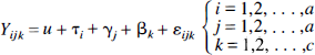
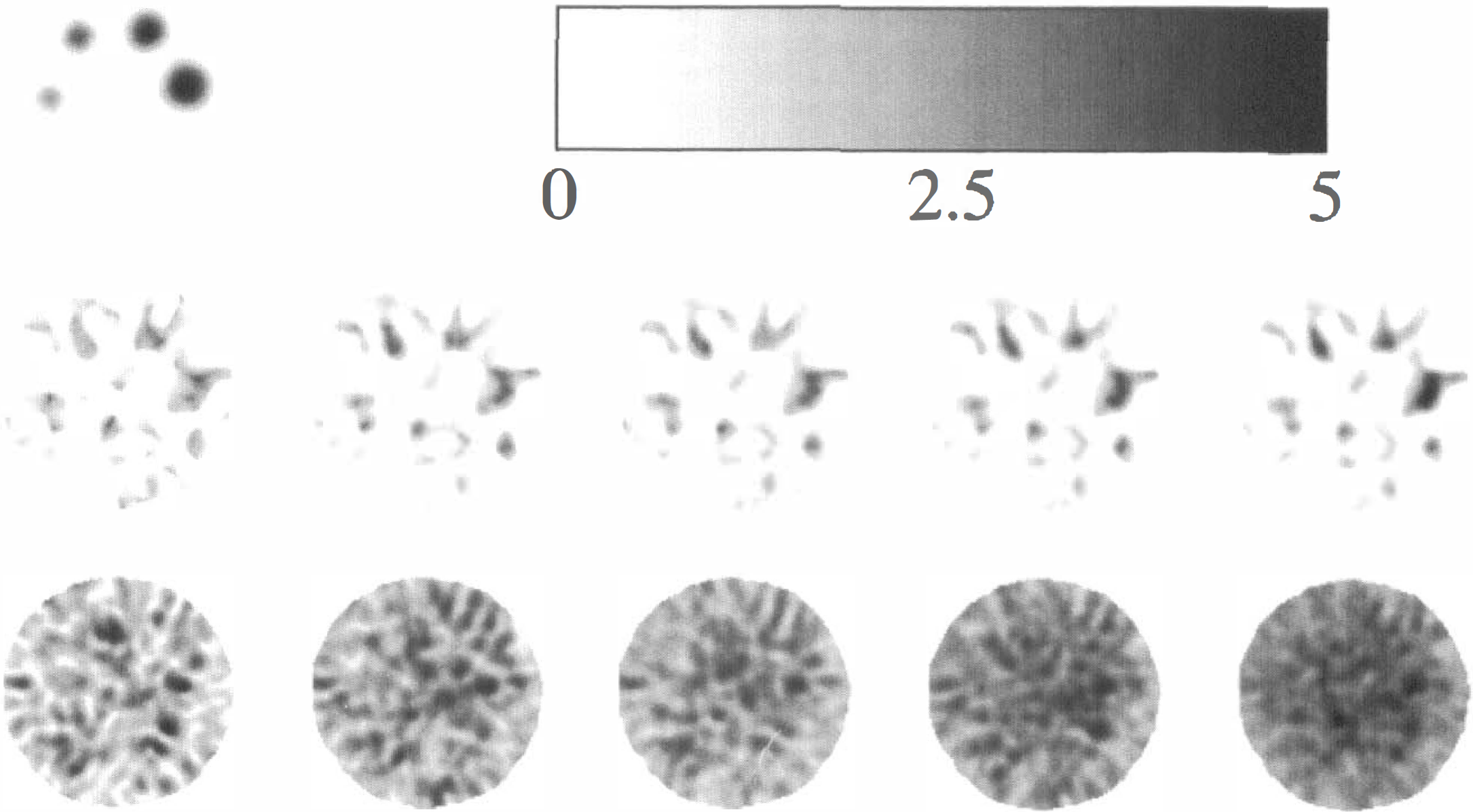
When dividing the data to represent a study in two subjects (df = 4), the t images displayed extreme fluctuations from close-to-zero MSE in some voxels (Worsley et al., 1993), and the significance (or more specifically, the effective resolution) could not be evaluated. The z score images and MSE1/2 images for all n values are presented in Fig. 1. Notice how the z score images get gradually better as data are divided into more frames, explained by the increased smoothness of the MSE1/2 images in the lower row. This specific slice for this specific contrast exhibits no extreme voxels in the z score image, but t values larger than 30 were found in all contrasts. The z scores for all spheres increased as number of subjects and degrees of freedom increased, and the peak P values decreased correspondingly. The cluster P values also decreased, but not as markedly as those based on the peak values. An example of the behavior of the peak and cluster P values is shown in Fig. 2. The error bars represent the minimum and maximum P value from the four contrasts examined and the markers represent their average.
Upper row: On the left is shown the true placement and size of the spheres in the phantom, and on the right is shown the z score gray scale for the images in the middle row. Middle row: The z score images obtained when dividing data into (from left to right) 2, 3, 4, 6, and 12 subjects (df = 4, 8, 12, 20, 44, respectively). Notice, for example, how the z scores for the largest sphere increase as the degrees of freedom increase. Lower row: MSE½ maps, each one scaled to its own maximum. Their smoothness increases with increasing degrees of freedom.
Examples of P values for two of the spheres (25.5 mm and 33 mm, respectively) estimated from peak value and spatial extent of cluster, respectively. The markers represent the mean, and the error bars the maximum and minimum of four independent realizations. The conventionally used significance level (P = 0.05) has been marked with a thick line in the graph. The existence of peak-based P values larger than 1 is because the value that is estimated is really the most likely number of peaks with this z score or larger, and only for small values does it asymptotically approach the probability of finding one or more peaks with this z score or larger (Friston et al., 1994).
Human study
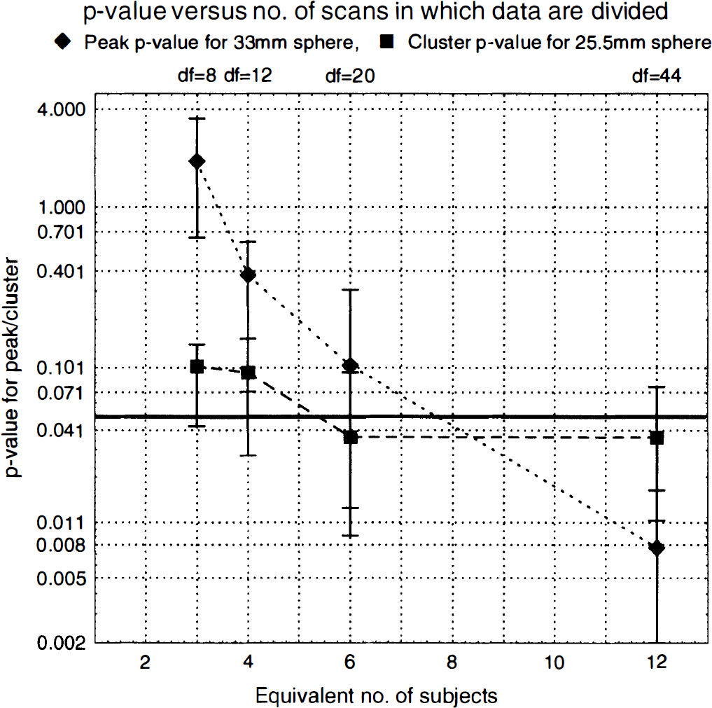
Examination of the MSE1/2 maps showed clearly that MSE was higher in central than in superficial areas, that MSE was higher in direct than cross-planes, and that it was higher in caudal slices where the head diameter was large than in cranial slices where head diameter was small. Results from ROI drawn in the MSE1/2 maps for two subjects are shown in Fig. 3 and demonstrate this clearly.
Spatial variation in residual error. (
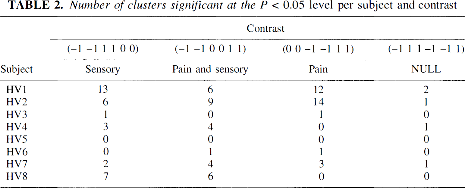
The results from the group-based analysis are presented in Table 1, and the statistics from the individual analysis are presented in Table 2 and Table 3. Results of the single-subject analysis will be fully reported elsewhere. Table 2 indicates that there are large intersubject differences in the number of detected regions, and also that the specificity was 0.62 (5/8) rather than the theoretically expected 0.05. However, as may be seen from Table 3, part of the intersubject differences are explained by coalescing of nearby situated clusters in some subjects (HV4 and HV7), whereas in others there were several separated clusters within the same anatomical structure (HV1 and HV2).
Results from group-based analysis
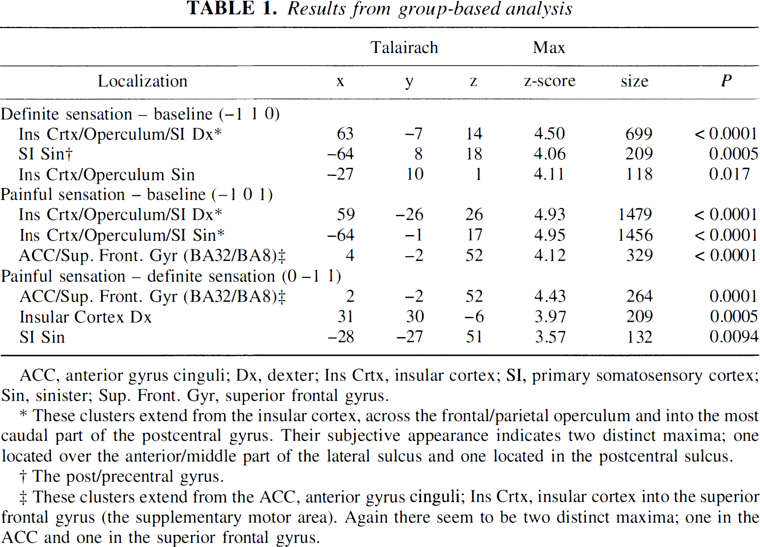
ACC, anterior gyrus cinguli; Dx, dexter; Ins Crtx, insular cortex; SI, primary somatosensory cortex; Sin, sinister; Sup. Front. Gyr, superior frontal gyrus.
These clusters extend from the insular cortex, across the frontal/parietal operculum and into the most caudal part of the postcentral gyrus. Their subjective appearance indicates two distinct maxima; one located over the anterior/middle part of the lateral sulcus and one located in the postcentral sulcus.
The post/precentral gyrus.
These clusters extend from the ACC, anterior gyrus cinguli; Ins Crtx, insular cortex into the superior frontal gyrus (the supplementary motor area). Again there seem to be two distinct maxima; one in the ACC and one in the superior frontal gyrus.
Number of clusters significant at the P < 0.05 level per subject and contrast
Activated clusters per area and subject
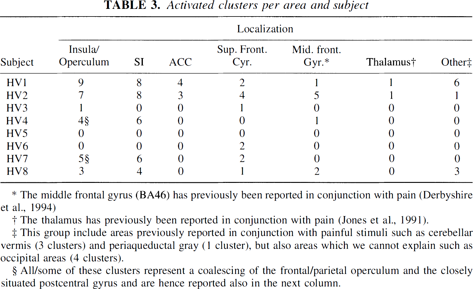
The middle frontal gyrus (BA46) has previously been reported in conjunction with pain (Derbyshire et al., 1994)
The thalamus has previously been reported in conjunction with pain (Jones et al., 1991).
This group include areas previously reported in conjunction with painful stimuli such as cerebellar vermis (3 clusters) and periaqueductal gray (1 cluster), but also areas which we cannot explain such as occipital areas (4 clusters).
All/some of these clusters represent a coalescing of the frontal/parietal operculum and the closely situated postcentral gyrus and are hence reported also in the next column.
An example of detected clusters in the contrasts (−1 −1 1 1 0 0) and (−1 −1 0 0 1 1) is shown for subject HV7 in Fig. 4 overlaid on the MR images from that subject. Mean and standard deviations, after correction for global flow and block effects, of the voxels with maximal z score for each activated area in subject HV7 are shown in Fig. 5. Examples of the residuals plotted versus predicted value, residuals plotted versus sequence number, and probability—probability plots (for the normal distribution) of the residuals are shown in Fig. 6 through 8, respectively. Plotting of residuals versus predicted value (Fig. 6) revealed no correlations, and the probability—probability plots (Fig. 7) did not indicate any systematic deviations from normal distribution. The residuals versus sequential frame number (Fig. 8) indicated no serial correlations. The same type of plots are shown for a “false-positive” result in the same subject, revealing no deviations there either (Fig. 9). The observed distribution of the Durbin-Watson d statistic adhered closely to the predicted one. The predicted values for the d statistic and the first serial correlation were 2.163 and −0.107, respectively, and the observed average across subjects and voxels (a total of 576 observations) was 2.152 and −0.103, respectively. The total number of voxels with P < 0.05 and P < 0.20 (one-tailed test checking only for positive serial correlations) was 27 and 123, respectively (predicted numbers: 28.7 and 115.2). An example of the observed distribution for subject HV7 is shown in Fig. 10.
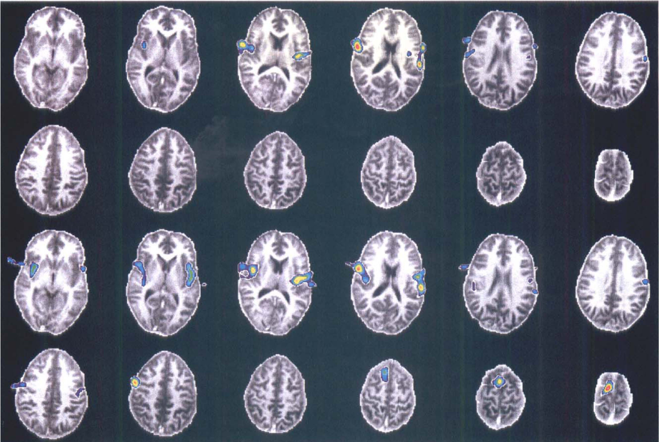
Upper two rows: Significant clusters for the definite sensation contrast (−1 −1 1 1 0 0) for subject HV7 overlaid onto his MR images. Lower two rows: Same as upper rows for the painful sensation contrast (−1 −1 0 0 1 1).
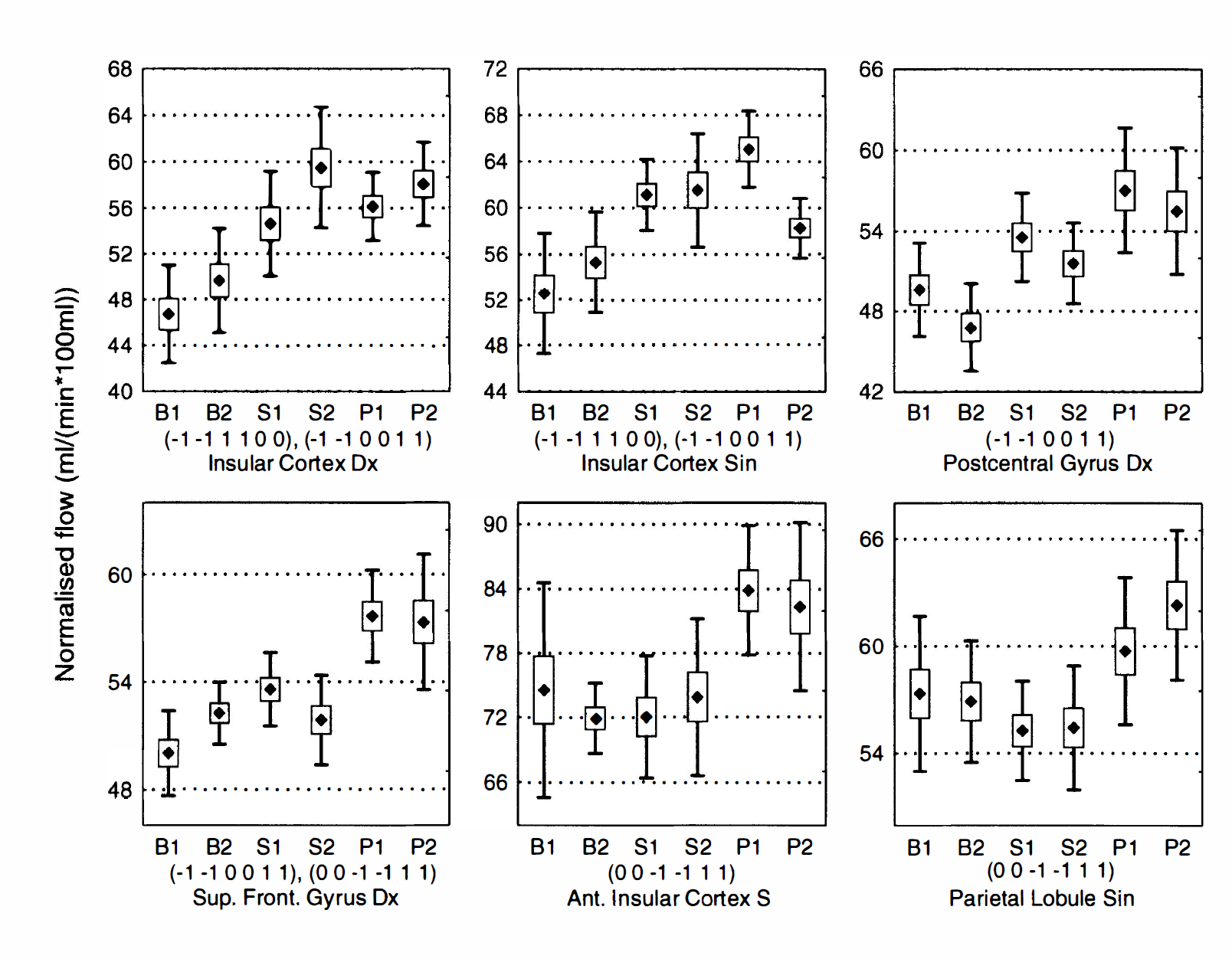
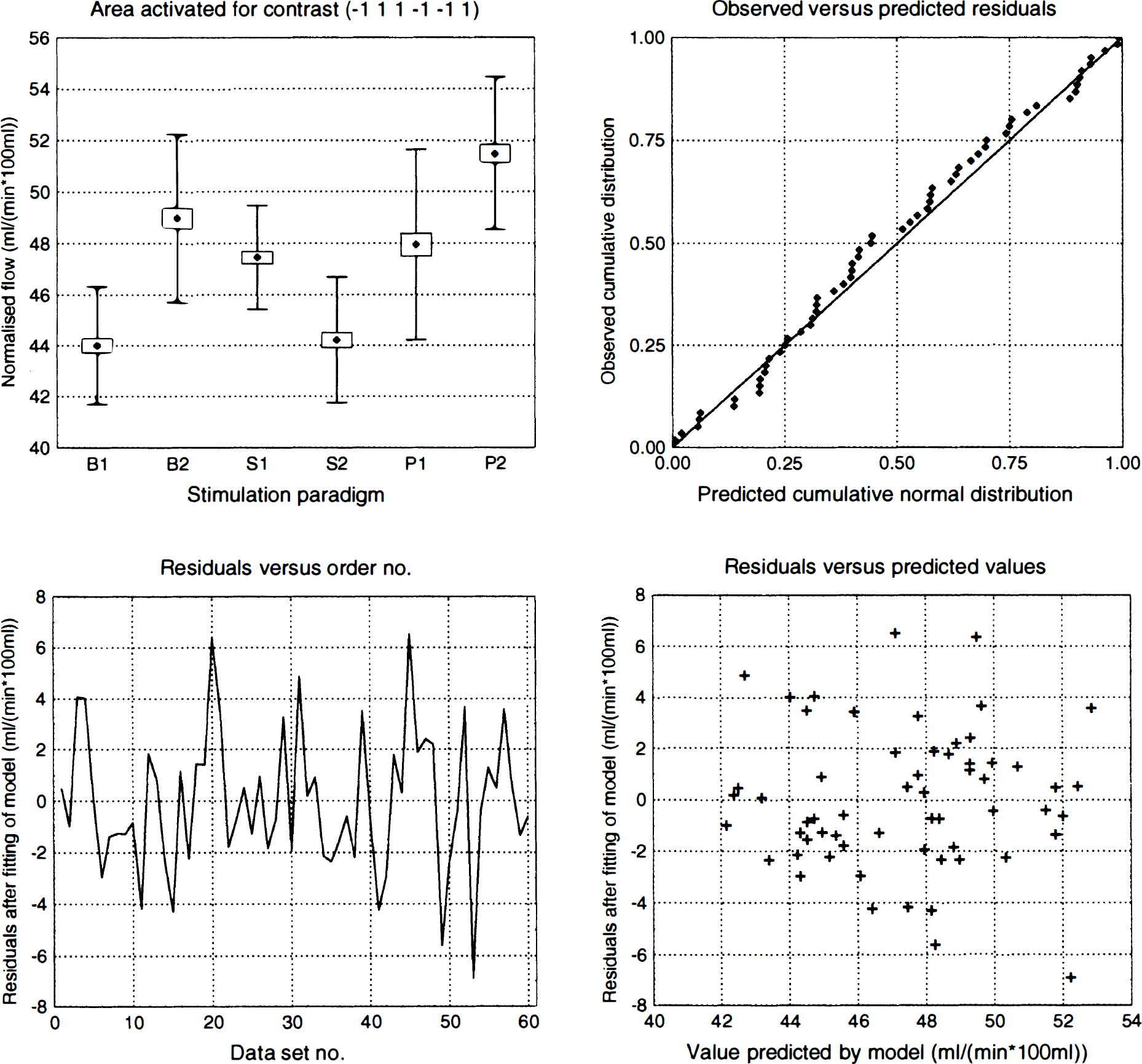
Activated areas in subject HV7. Mean (marker), standard error of the mean (box), and standard deviation (whiskers) for the voxel with the highest z score within each significantly activated cluster for subject HV7. States are labeled B1, B2 (baseline), S1 S2 (definite sensation), and P1 and P2 (painful sensation), and the contrasts for which the cluster was deemed as significant are indicated below each graph.
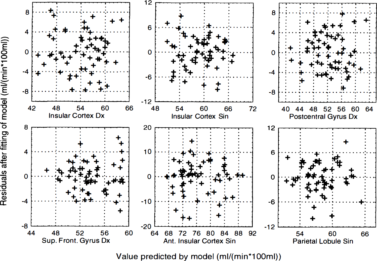
Residuals versus predicted values for activated areas in HV7. Residuals after fitting to the statistical model plotted versus value predicted by the model for all areas significantly activated in one or more contrasts in subject HV7. A curvilinear dependence in a plot of this kind indicates an inadequate statistical model (e.g., lack of an interaction term), whereas a funnel-shaped appearance of the plot indicates that the error variance is not constant. There are no clear patterns to indicate any such violation of the assumptions.
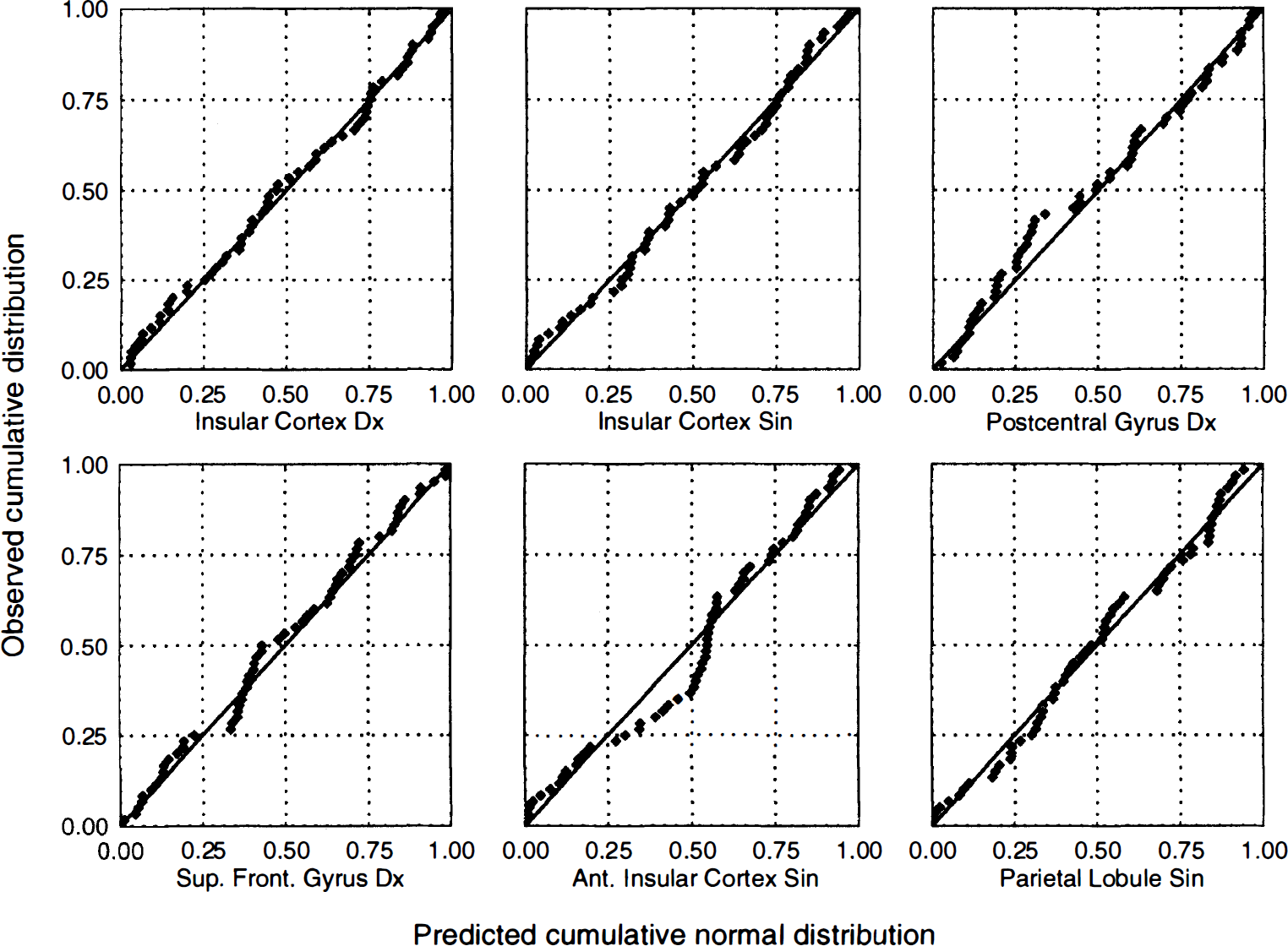
Predicted versus observed residuals for activated areas in HV7. Probability−probability plots of the residuals after fitting of the statistical model to all areas significantly activated in one or more contrasts in subject HV7. The plots are constructed by estimating μ and σ for a Gaussian distribution from the data at hand, and by plotting the observed cumulative distribution versus the theoretical [Gaussian distribution.] A perfect normal distribution would yield values along the identity line, whereas deviations from normal distribution would be expected to produce curved or S-shaped plots. No obvious deviations from the normality assumption could be found for these areas.
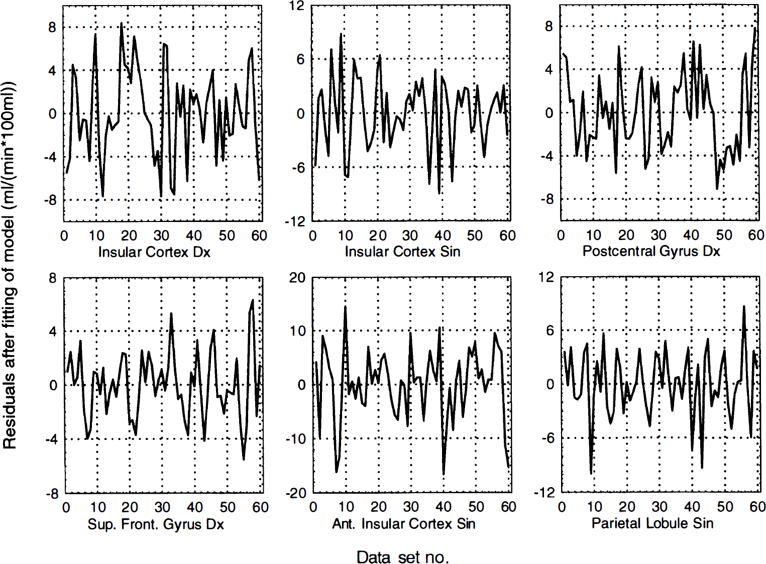
Residuals versus order number for activated areas in HV7. Residual after fitting of statistical model versus sequential scan order for all activated areas in subject HV7. The residuals are divided into sets of 10, where the first baseline scan constitutes the first 10 residuals, the second baseline scan constitutes the next 10 residuals, and so on. No obvious serial correlations could be found either by visual inspection or the Durbin-Watson test.
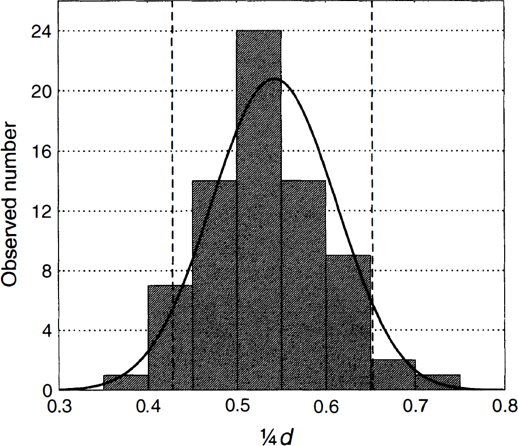
Observed (histogram) and predicted (solid line) distribution of 1/4 times the Durbin-Watson d statistic for 72 observations in HV7. Dotted vertical lines show the theoretical P = 0.05 levels (single-sided test). Observed and predicted number of voxels outside of the 0.05 and 0.20 levels at the lower end of the distribution (indicating positive serial correlation) were 4 and 17 versus 3.6 and 14.4, respectively, and at the upper end of the distribution, they were 3 and 12 versus 3.6 and 14.4, respectively. The expected values for d and r were 2.163 and −0.107, and the observed values were 2.128 and −0.089 respectively.
DISCUSSION
It is possible to perform a single-subject analysis, with a local variance estimate, of a PET activation study by dividing data obtained after a single injection into several frames. The main message in this report is that alternative data-collection strategies may yield more degrees of freedom when assessing statistical inference in activation studies. However, it is not suggested that the data-collection scheme used in the current study is the optimal one. There are two main objections that may be raised against our current design. First, the constant data collection time for each frame in the presence of the rapid decay of 15O yield poorer counting statistics for the latter frames, thereby invalidating the assumption of homoscedasticity. Although the analysis of residuals failed to demonstrate this effect, it is bound to be there to some extent. Second, the dynamics of H215O in the brain makes it necessary to adopt a blocked design, and that still does not address the problem of activation effect changing with time (Andersson and Schneider, 1997), for which an interaction term would need to have been included. However, the latter effect was at least partially counteracted in this experiment by discontinuing the stimulation when the activity had peaked in the brain (Volkow et al., 1991; Cherry et al., 1995).
A better design would be to collect an equal number of counts in each frame, and to let each frame represent the same period after injection of tracer. This may be roughly achieved by collecting data in a gated histogram mode, a method sometimes employed for cardiac studies, where data are gated with an ECG signal (Hoffman et al., 1979). For the current application, collection may be gated with an external clock pulse (one to a few hertz) and divided into a number of frames. The suitable number of frames would need to be determined, especially for the three-dimensional situation, where data storage and reconstruction times are issues. It would seem reasonable to aim for 40 to 50 df for the planned statistical design and to adjust the number of frames accordingly.
Phantom study
The phantom study was intended to demonstrate that how a given set of data with a given number of noise equivalent counts is divided actually makes a difference. The experiment was not intended to validate the strategy for single- or multiple-subject studies. This can be done on only human data, where the full complexity of tracer kinetics, between-injection differences in activation, and confounding unrelated activations is present. It did, however, clearly show that the z scores increased and the P values decreased as data were divided into more frames.
Human study
The examinations of the MSE1/2 maps demonstrated that the use of an error estimate based on pooling across all intracerebral voxels, (Worsley et al., 1991; Poline and Mazoyer, 1993; Knorr et al., 1993) which is another way to increase degrees of freedom and facilitate single-subject analysis, would be a poor approximation. The observed effects are easily explained by physical factors, where fewer counts are detected from central areas because of attenuation, where caudal slices with large head diameters also are subject to more attenuation than more cranial slices, and where more counts are collected in cross-planes than in direct planes because of geometric factors (Holte et al., 1989). The latter effect would not be observed in a septaless three-dimensional scanner, but the larger actual acceptance angle for the middle slices instead would produce a larger MSE for the extreme slices at both ends of the scanner (Cherry et al., 1991).
Interestingly, in a recent study (Andersson et al., 1995a), we examined the residuals obtained from a group-based analysis and failed to detect these (expected) effects. Clearly, the difference between direct planes and cross-planes is lost in the stereotactical normalization process; more surprisingly, the depth effects from attenuation also are lost. The residuals obtained with the current method result mainly from counting statistics, whereas in a group-based analysis, intersubject differences in activation are likely to be a major source of variation. Taken together, the results from the current study and our previous work (Andersson et al., 1995a) indicate that intersubject differences in activation dominate the error term to the extent that regional variations in the counting statistical contributions to the error can no longer be detected.
The results from the group-based analysis indicate several areas for the sensory and painful states (Table 1), whose neurophysiologic relevance is discussed in another report (Aziz et al., 1997). The results are in no way unreasonable and adhere to what has been previously known about processing of visceral sensation (Cechetto and Saper, 1990) and painful stimuli in general (Hsieh, 1995).
The single-subject analysis yielded results with a large intersubject variability with respect to number of activated areas, where in some subjects (HV1 and HV2) most of the areas implied by the group-based analysis were detected, whereas in others no or few areas were found (HV3, HV5, and HV6). When examining the actual increases in activity (data not shown) in significant clusters, increases larger than 15 mL/(min · 100 mL) (normalized activity) were typically found in the caudal slices and larger than 10 mL/(min · 100 mL) in the cranial slices. Even when performing a hypothesis-driven manual search for activated areas in subjects HV3, HV5, and HV6, no areas with increases of this magnitude were obvious. Hence, it seems likely that the results represent an absence of activations of the necessary magnitude.
The poorer than expected specificity may be caused by several factors. First, the assumption of statistical independence between frames may be wrong. Second, the methods used for assessment of significance are based on several assumptions and have not been experimentally verified (Friston et al., 1994). Third, when performing a single-subject analysis, order effects are not balanced out, and other factors such as mood shifts, discomfort, and uncontrolled thoughts are not dispersed, as is the case in a group of subjects.
The first factor has been extensively examined in the preparation of this report, and there are no indications of any violations. To examine the second factor is beyond the scope of this report, and other studies are needed to determine this. I favor the third factor as the most likely explanation for the observed frequency of type 1 errors, and a further discussion of this is found later in this report.
Statistical independence of frames
Realize that the question of statistical independence must be put in relation to the desired inferences. When performing a single-subject experiment in the manner suggested in the current report, inferences are made regarding the differences between two or more scans, in which case statistical independence between frames is a reasonable assumption, and the method may be viewed as a way of putting a counting statistical error bar on each voxel. On the other extreme, it has been suggested that to make inferences regarding the entire population based on experiments performed in a group of limited size, it is not correct even to consider data from consecutive injections as independent (Woods et al., 1996). For example, when analyzing an 8 × 2 × 3 (eight subjects, two tasks, three replications) study using a two-way ANOVA/ANCOVA, the residuals within each block of three replications certainly will be strongly correlated. Whether this is to be viewed as a deterministic effect or a violation of statistical independence depends on what type of conclusion is attempted.
Related work
There has been previous attempts to obtain a reasonably reliable counting statistical error estimate, hence facilitating single-subject studies. Some workers have pooled the error estimate in the spatial domain (Poline and Mazoyer, 1993; Knorr et al., 1993) but, as evident from Fig. 3, that is not a valid approach. An alternative strategy was suggested by Cherry and others (1993b) and subsequently refined by Votaw and Li (1995). That method generates z score sinograms by assuming Poisson statistics in the uncorrected sinograms, and proceeds to reconstruct z score images directly. The results should be comparable with those obtained with the method suggested in the current report. An advantage with those methods (Cherry et al., 1993b; Votaw and Li, 1995) is that data storage and reconstruction times remain essentially unchanged. A disadvantage is the need to write or modify reconstruction software, whereas the method suggested in the current report may be used directly with the commonly available statistical parametric mapping software.
Possibilities
It is not suggested that this method should motivate the use of smaller groups in activation studies, nor that it should replace the current group-based methods of analysis. It is suggested as a valuable complement that may help to demonstrate between-subject differences in activation and identify subgroups with different strategies to a given problem (Fiez et al., 1996).
It may further facilitate activation studies in the presence of disease, where group-based analysis is problematic because of possible intersubject differences in degree and localization of the pathologic process (Chollet et al., 1991). It also may be a valuable tool for the analysis of single-subject studies aimed at determining the localization of functionally important areas before surgery (Leblanc and Meyer 1990; Pardo and Fox 1993).
More elaborate statistical models for which intersubject differences in activation are accounted has been suggested (Woods et al., 1996). These would potentially increase sensitivity by lowering the MSE in activated areas, but also would be penalized with lower degrees of freedom. This may be counteracted by dividing each injection into two or more frames, thereby restoring degrees of freedom. In this case, the alternative data-collection strategy suggested earlier (gated by an external clock) would be advantageous because it would eliminate the need for frame number as an additional block direction.
Another area where the current method may potentially be useful is when performing activation studies with more long-lived isotopes. For example, when studying neuromodulation with 11C-labeled tracers (Morris et al., 1995; Fisher et al., 1995), it would be costly and time-consuming to collect an adequate number of studies to yield 30 or more degrees of freedom. The strategy suggested in this report may be a way to yield interpretable results from a reasonably sized and priced study.
Dangers
Care should be taken not to overinterpret the results from an analysis of the suggested type. When considering a group-based analysis, the residual error will originate from three sources: intersubject differences in activation (localization and magnitude), intrasubject differences (such as time effects and confounding activations not possible to control for), and counting statistical noise. When considering a single-subject study in which numerous injections (16–24) have been performed, the error sources will be restricted to the two latter ones. Finally, when performing an analysis of the kind suggested in the current report, the error term will be completely dominated by counting statistics.
This has important implications for the interpretation of the results. When an area is deemed significant with the current method, it means that there is a significant difference between these specific PET scans. However, it does not mean that the difference is with certainty caused by the activation paradigm. Confounding factors such as time effects, which normally are balanced across a group, or lack of control over a subject's thoughts, which may be considered to even out across a group, enter directly into the results.
For this reason, the quoted significance level (normally P < 0.05) should be interpreted as the significance level for these specific data sets, and not as a significance level necessarily related to the activation paradigm. The mismatch between the theoretical and the observed specificity found in the human material may result from such considerations. Indeed, the subject (HV1) with two significant clusters in the NULL contrast, as well as a couple of activated areas during the other contrasts that did not match the results from the group analysis, could be expected to have been in emotional turmoil caused by events unrelated to the PET scanning.
CONCLUSION
Here I suggest the use of multiple frames after a single injection and demonstrate its usefulness for single-subject studies. These ideas will be pursued further in future work with special attention to activation/perturbation studies with 11C-labeled ligands.
Footnotes
Abbreviations used
Acknowledgments
The author thanks Drs. Qasim Aziz and David Thompson for supplying the data from the human study used in the evaluation of the method.