Analysis of Dynamic Radioligand Displacement or “Activation” Studies

Abstract

We present a simple way of assessing dynamic or time-dependent changes in displacement during single-subject radioligand positron emission tomography (PET) activation studies. The approach is designed to facilitate dynamic activation studies using selective radioligands. These studies are, in principle, capable of characterising functional neurochemistry by analogy with the study of functional neuroanatomy using rCBF activation studies. The proposed approach combines time-dependent compartmental models of tracer kinetics and the general linear model used in statistical parametric mapping. This provides for a comprehensive, voxel-based and data-led assessment of regionally specific effects. The statistical model proposed in this paper is predicated on a single-compartment model extended to allow for time-dependent changes in kinetics. We have addressed the sensitivity and specificity of the analysis, as it would be used operationally, by applying the analysis to ¹¹C-Flumazenil dynamic displacement studies. The activation used in this demonstration study was a pharmacological (i.v. midazolam) challenge, 30 min after administration of the tracer. We were able to demonstrate, and make statistical inferences about, regional increases in k₂ (or decreases in the volume of distribution) in prefrontal and other cortical areas.

This report describes the analysis of single-subject dynamic radioligand displacement studies using positron emission tomography (PET) or, more colloquially, hot ligand activation studies. Dynamic studies using H₂¹⁵O to measure evoked changes in rCBF are now firmly established as a powerful method in the study of functional neuroanatomy. The idea behind dynamic radioligand displacement is that endogenous changes in neurotransmitter release, or exogenous administration of centrally acting drugs, can be characterised by examining the time-dependent displacement of “hot” ligands that might ensue. The specificity of this new technique is implicit in the receptor specificity of the radioligand used. The potential importance for a mechanistic understanding of functional neurochemistry and psychopharmacology is clearly enormous.

In general, there are two approaches to measuring occupancy changes of displaceable PET radioligands induced by exogenous administration of competing ligands or by endogenous release of neurotransmitters. The first approach assumes equilibrium conditions (e.g., using competitive agonists/antagonists with long half-lives or a continuous infusion) and compares two scans, with and without a challenge, to test for differences in equilibrium kinetics. The second approach is to perturb the displacement kinetics dynamically with a challenge (e.g., Brouillet et al., 1991; Delforge et al., 1995) and assess the degree of perturbation. This assessment can use two dynamic scans, with and without perturbation (see Morris et al., 1995, for an excellent analysis of how to optimize the design of two-scan procedures and a discussion of the issues that ensue) or can proceed using a single time-series using the evoked changes in kinetics. This paper is concerned with the latter approach to studying endogenous activation.

The aim of this paper is to describe a method that allows statistical inferences about dynamic or time-dependent changes in tracer kinetics, attributable to some challenge, using a single injection of radioligand. The nature of the challenge can vary, for example, sensory stimulation, specific cognitive activation, motor performance or learning, sensorimotor integration, and pharmacological or neuroendocrine challenge. The changes in tracer kinetics following the activation will be referred to as time-dependent changes that are attributed to the activation. To demonstrate the method clearly we have chosen a simple example with a clear positive result. The radioligand used was ¹¹C-Flumazenil. The activation was a pharmacological challenge with unlabelled i.v. midazolam. This experiment was designed to ensure time-dependent changes in tracer kinetics.

Provided the input function is estimated adequately, changes in kinetic parameters can be estimated using pharmacokinetic models (e.g., Cunningham and Jones, 1993); however, there is no satisfactory method for making statistical inferences about these effects, independently of a separate control study (without an “activation”). There are many potentially confounding differences between a dynamic displacement and a control study, for example, alignment differences, different input functions, order effects, differences in the physiological response and baseline, and so on. We therefore concentrated on the problem of making inferences about dynamic changes in kinetics using just the one activation study while acknowledging the importance of two-scan procedures and the fact that many of these issues also confound single-scan designs.

¹¹C-Flumazenil is a well-established PET ligand that is used in the study of central benzodiazepine receptors (Maziere et al., 1984; Ehrin et al., 1984). Flumazenil is an ideal ligand in the sense that it is highly specific for the benzodiazepine-GABA-A complex and can be administered in doses that produce a significant degree of receptor occupancy without clinical effects. It is rapidly metabolised, outside the brain, to a hydrophilic molecule that does not cross the blood–brain barrier. It shows reversible binding and has low levels of nonspecific binding (Abadie and Baron, 1991). Flumazenil demonstrates a simple kinetic behaviour in the brain that conforms (nearly) to a single-compartment model (Koeppe et al., 1991). For a single-compartmental model, gray matter clearance rates have a half-life of about 700 s and a maximal V_d of about 7 ml/ml. Estimates of B_max and K_d suggest that the cortex (particularly the occipital and prefrontal) express the greatest binding potential with lower values for the basal ganglia, cerebellum and brainstem (Lammertsma et al., 1993).

The paper is divided into four parts: theory, validation, application, and discussion. The theory sections describe intuitively and mathematically the tenets of the analysis. The proposed method tries to bridge the gap between parameter estimation in pharmacokinetic models, for example, spectral analysis (Cunningham and Jones, 1993) and nonlinear least squares, and the general linear model used in statistical parametric mapping. The validation and application sections describe the data and study protocol, spatial (stereotactic) normalisation, and subsequent analysis. The validation section uses a study with no activation to ensure that the statistical distributions of various terms behave as expected under the null hypothesis. The application section considers the analysis of a single activation study. The discussion focuses on how the minimal model, presented in previous sections, can be generalised and some of the limitations of the approach.

The empirical results in this paper are presented as a “demonstration” study; the neurobiological implications and interpretations will be communicated separately on the basis of a larger study. In particular, the results should not be taken as a validation of the proposed technique per se but serve only as an illustration of the idea, its procedural aspects, and how to address issues of validity.

THEORY

In the following sections, we describe the statistical model used in our analysis, the derivation of kinetic parameters, and how to make statistical inferences about time-dependent changes in displacement on a voxel-by-voxel basis. The approach brings together three well-established bodies of theory: the modelling of tracer kinetics, the general linear model, and the theory of Gaussian fields. This represents an attempt to combine pharmacokinetic modelling and statistical parametric mapping.

There is an important distinction between a pharmacokinetic model or, more generally, biomathematical models and statistical models: The aim of biomathematical models (e.g., compartmental models, synthetic neural models, and so on) is to emulate the behaviour of a biological system, either to reproduce some emergent phenomena or to facilitate parameter estimation. The structure of the model is chosen to have the greatest validity in reference to the system modelled. In contrast, the aim of a statistical model is to maximize the sensitivity or power to detect some effect of interest. The nature of this effect and the associated parameter estimates are of secondary importance (and could be explored post hoc with biomathematical models). Unlike other models, statistical models must satisfy several specific constraints: One important constraint is the explicit inclusion of a well-behaved error term, the variance of which can be estimated. The more degrees of freedom available for this estimation, the more powerful the statistical inference that ensues. Generally speaking, simpler models (models with few parameters) are more powerful because every parameter of the model “uses up” a degree of freedom, which means that a statistical model of tracer kinetics must be very constrained or specified with few parameters. The statistical model described below is linear, requires only a small number of estimated parameters, retains a reasonable relationship to the underlying time-dependent compartmental model, and renders the data and error terms appropriately distributed under the null hypothesis.

The basic idea

This section provides an intuitive idea of how the analysis proceeds. The general strategy is described, followed first by a more formal description of a “minimal” example. This example is then used in the analysis of empirical data.

1. First identify a set of differential (or difference) equations that characterise the generally multicompartment time-dependent model appropriate for the kinetics under study. Unlike conventional pharmacokinetic models, some terms usually considered as rate constants will be functions of time [e.g., k₂(t) as opposed to k₂]. These functions are parameterised by expanding in terms of appropriate temporal basis functions (e.g., Fourier expansion, polynomial expansion, or some arbitrary set of time-dependent curves). The coefficients of these expansions now constitute the parameters of the model. One or more of these coefficients will model the dynamic effect of interest and, under the null hypothesis, will be zero.

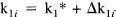
2. Identify normal or expected values for all the parameters (e.g., k₁, k₂, and so on). Integrate the differential equations above to obtain a normal or “canonical” tissue activity curve and corresponding counts per frame (observed activity).

3. By applying a small change to each of the parameters in turn, estimate the partial derivative of the canonical activities with respect to each parameter. This step is most simply effected by reintegrating the difference equations and subtracting the canonical form from the result.

4. The observed counts per frame will, to a first-order approximation, be the sum of the canonical form and, for each parameter, the difference between the actual parameter and its expected value times the appropriate first derivative. This approximate equality allows one to linearise the problem and express it in terms of the general linear model: First subtract the canonical form from the observed values at each voxel. After appropriate weighting (to account for Poisson statistics), these corrected counts now constitute the response variable, which is, disregarding error terms, the sum of all the deviations of each parameter from the expected value, times the respective (weighted) partial derivative. These deviations are now estimated in a least-squares sense using the response variables at each voxel and the (weighted) matrix of partial derivatives.

5. The effects of interest are modelled by the coefficients of the expansions describing time-dependent changes in specific variables (e.g., k₂ or k₄). The null hypothesis, that these coefficients are zero, is tested with the F or t statistic using the sum of squares due to the effects (parameters) we are interested in and the sum of squares due to error.

6. The resulting image of F or t statistical quotients is now subject to standard procedures developed for statistical inference in statistical parametric mapping.

In the next section, we consider a simple example of this general approach using a single-compartment model with a single form of time-dependent change in one kinetic parameter (k₂). This minimal model is the model used in the analysis of the empirical data.

The statistical model: An example

In this section, we present the statistical model used to assess the degree and significance of dynamic changes in kinetics during a ¹¹C-Flumazenil study. Because a single compartment (monoexponential) model is sufficient to describe the tissue dynamics of ¹¹C-Flumazenil (Koeppe et al., 1991), the corresponding statistical model was based on a single compartment. The observed variable F_ij corresponds to the tissue activity (per frame) measured at voxel i in frame j:

$F_{ij}=\int C_{\mathrm{i}}(t)+{\mathrm{V}}_{\mathrm{b}}{C}_{\mathrm{b}}(t)dt+{(W_j)}^{1/2}(r_{ij}+{\mathrm{o}}_i)$

(1)

where scan j starts at time t_j and finishes at t_j+1 and the integral is over this period. C_b(t) is the whole blood activity at time t, and V_bC_b(t) represents the small contribution to the measured activity from the blood compartment with volume V_b (fixed at 0.1 for all voxels). (W_j)^1/2 (r_ij + o _i ) is a residual term appropriate for Poisson statistics, where W_j is the whole brain activity for scan j, and r_ij is assumed to be identically and independently distributed as N(0, σ²); o _i is a small, constant background term. The time-dependent tissue activity C_j(t) is given by the differential equation:

$d{C}_i(t)/dt={\kappa }_{1i}\hspace{0.17em}{\mathrm{C}}_{\mathrm{p}}(t-{\delta }_i)-{\kappa }_2{(t)}_i+\lambda ).C_i(t)$

(2)

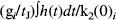
κ_1i is the plasma to tissue transfer rate for voxel i. C_p(t – δ _i ) is the metabolite corrected plasma curve, or delayed input function, and δ _i is the delay incurred by its estimation in the periphery relative to brain region i. An example of C_p(t) is shown in Fig. 1 (upper panel). These data were obtained from the validation study described in a subsequent section. λ is the radiodecay parameter for the tracer (in this case, 0.0005663 s^–1). κ₂(t) _i corresponds to the rate of clearance from the tissue compartment for voxel i at time t. The clearance κ₂(t) _i is a time-dependent variable that may exhibit changes due to the activation [note that time-dependent changes in κ_1i would have little impact later in the study because C_p(t – δ _i ) will be small]. It is these activation-induced changes that we are interested in: Let κ₂(t) _i be expanded in terms of some regionally invariant “normal” value (κ₂*), a region or voxel-specific effect (Δκ_2i), and a voxel-specific, time-dependent component due to the activation Γ _i (t). The dynamic component due to changes in displacement Γ _i (t) can be expressed in terms of some appropriate function of time, say, h(t) so that Γ _i (t) = γ_i · h(t) (see Discussion for a more general expansion). The form of h(t) defines the time course of displacement dynamics about which one wants to make inferences. In this paper, we assume that the effect of the activation is to induce a fairly protracted increase in displacement κ₂ or equivalently a decrease in the volume of distribution (see below). The coefficient γ_i is the unknown that represents this effect of interest and under the null hypothesis of no time-dependent displacement γ_i = 0:

${\kappa }_2{(t)}_i={\kappa }_2*+\Delta {\kappa }_{2i}+{\gamma }_i.h(t)$

and similarly

$\begin{array}{lll}{\kappa }_{1i}\hfill & =\hfill & {\kappa }_{1\hspace{0.17em}}*+\hspace{0.17em}\Delta {\kappa }_{1i}\hfill \\ \hspace{0.17em}\hspace{0.17em}{\delta }_i\hfill & =\hfill & {\delta }^{*}+\Delta {\delta }_i\hfill \end{array}$

(3)

FIG. 1.

Upper panel: Whole blood C_b(t) and input function or metabolite corrected plasma activity C_p(t) as a function of time. These data were based on whole-blood activity monitored every second. The whole-blood data were transformed and metabolite corrected on the basis of discrete arterial samples. Lower panel: A typical curve for the canonical form of measured counts per frame. This curve was obtained by using C_b(t) and C_p(t) shown in the upper panel and assumes 64-s time frames throughout the study. Values for parameters were as follows; κ₁* = 0.0077/s, κ₂* = 0.0045/s, δ* = 16 s, V_b = 0.1 and λ = 0.0056/s.

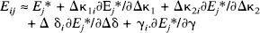
For ¹¹C-Flumazenil, we could assume a value of κ₂* that is typical of gray matter (e.g., 0.0045) or estimate κ₂* by using the whole brain curve for the study in question and similarly for κ₁* and δ*. Combining Eqs. 1, 2, and 3, we can express expected activity at voxel i in frame j, (E _ij ) as a function of four unknown parameters:

${\mathrm{E}}_{ij}(\Delta {\kappa }_{1i},\Delta {\delta }_i,\Delta {\kappa }_{2i},{\gamma }_i)=\int C_i(t)+{\mathrm{V}}_{\mathrm{b}}{\mathrm{C}}_{\mathrm{b}}(t)dt$

(4)

Integrating over the time of the frame. If we make the simplifying assumption that the deviations from the canonical values (Δκ_1i, Δδ _i , Δκ_2i, γ_i) at each voxel are small, we can take a first-order approximation of a Taylor expansion of E_ij around E _j * = E_ij(0, 0, 0, 0) where

$\begin{array}{lll}{E}_{ij}\hfill & \approx \hfill & \hspace{0.17em}\hspace{0.17em}\hspace{0.17em}{E}_j*+\Delta {\kappa }_{1i}\partial {\mathrm{E}}_j*/\partial \Delta {\kappa }_1+\Delta {\kappa }_{2i}\partial E_j*/\partial \Delta {\kappa }_2\hfill \\ \hfill & \hfill & +\Delta \hspace{0.17em}\hspace{0.17em}{\delta }_i\partial E_j*/\partial \Delta \delta +{\gamma }_i.\partial E_j*/\partial \gamma \hfill \end{array}$

(5)

A typical curve for the canonical form is shown in Fig. 1 (lower panel). This curve was obtained by using C_b(t) and C_p(t), shown in the upper panel of Fig. 1, and assuming 64 second time frames throughout the study. Values for each of the parameters were as follows; κ₁* = 0.0077 per second, κ₂* = 0.0045 per second, δ* = 16 second, V_b = 0.1 and λ = 0.0056/s.

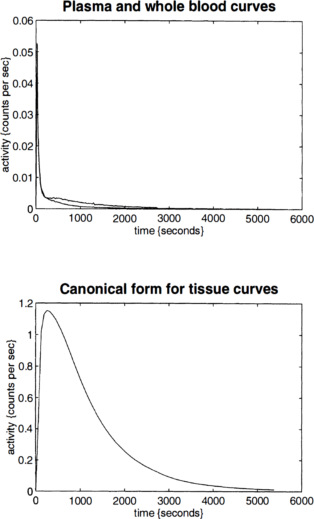
In practice, E _j * and the partial derivatives are most simply obtained by numerical integration of Eq. 3: For example, the partial derivative ∂E_j*/∂Δκ₁ is estimated with [E_ij(p, 0, 0, 0) – E_ij(0, 0, 0, 0)]/p, where p is some suitably small perturbation. Examples of these partial derivatives are presented in Fig. 2. The upper panel shows the partial derivatives with respect to Δκ_1., Δδ, and Δκ₂. These profiles can be thought of as the deviation from the canonical form in Fig. 1 that would ensue if Δκ_1i, Δδ _i , or Δκ_2i changed slightly. The fourth partial derivative ∂E_j*/∂γ modelling a time-dependent increase in κ₂ is seen in the lower panel of Fig. 2 (solid line). The assumed form for changes in κ₂ is superimposed (broken line) and corresponds to h(t). A transient increase in κ₂ produces an accelerated decay in observed counts; it is this perturbation of the dynamics that the model is designed to assess. The curves have been scaled to allow comparisons among them.

FIG. 2.

Upper panel: Examples of the partial derivatives with respect to Δκ, Δδ, and Δκ₂. These profiles can be thought of as the deviation from the canonical form in Fig. 1 (lower panel) that would ensure if Δκ_1i, Δδ _i , or Δκ_2i. changed slightly. Lower panel: The fourth partial derivative ∂E _j */∂γ modelling a time-dependent increase in κ₂ (solid line). The assumed form for changes in κ₂ is superimposed (broken line) and corresponds to h(t). A transient increase in κ₂ produces an accelerated decay in observed counts; h(t) is a Gaussian curve (of parameter 64 s) centred at 2,100 s and convolved with an exponential function with a half-life of 320 s (5 min).

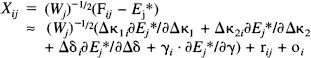
Combining Eqs. 1 and 5, we can now define the response variable X_ij as:

$\begin{array}{lll}{X}_{ij}\hfill & =\hfill & {(W_j)}^{-1/2}({\mathrm{F}}_{ij}-E_{\mathrm{j}}*)\hfill \\ \hfill & \approx \hfill & {(W_j)}^{-1/2}(\Delta {\kappa }_{1i}\partial E_j*/\partial \Delta {\kappa }_1+\Delta {\kappa }_{2i}\partial E_j*/\partial \Delta {\kappa }_2\hfill \\ \hfill & \hfill & +\hspace{0.17em}\Delta {\delta }_i\partial E_j*/\partial \Delta \delta +{\gamma }_i\cdot \partial E_j*/\partial \gamma )+{\mathrm{r}}_{ij}+{\mathrm{o}}_i\hfill \end{array}$

In matrix notation:

${\mathrm{X}}_i\approx \mathrm{G}\cdot {\beta }_{\mathrm{i}}+{\mathrm{r}}_{\mathrm{i}}$

where

${\mathrm{X}}_i=\text{diag}{(\mathrm{W})}^{-1/2}\cdot ({\mathrm{F}}_i-{\mathrm{E}}^{*})$

and

$\begin{array}{lll}\mathrm{G}\hfill & =\hfill & \{1\hspace{0.17em}\hspace{0.17em}{\text{diag}(\mathrm{W})}^{-1/2}\cdot [(\partial \mathrm{E}*/\partial \Delta {\kappa }_1)\hfill \\ \hfill & \hfill & \times (\partial \mathrm{E}*/\partial \Delta {\kappa }_2)(\partial \mathrm{E}*/\partial \Delta \delta (\partial \mathrm{E}*/\partial \gamma )]\}\hfill \end{array}$

and

${\beta }_i={[{\mathrm{o}}_i,\Delta {\kappa }_{1i},\Delta {\delta }_i,\Delta {\kappa }_{2i},{\gamma }_i]}^{\mathrm{T}}$

(6)

Eq. 6 is the general linear model with design matrix G (see Chatfield and Collins, 1980). X_i is a column vector of the response variables (counts per frame corrected for the canonical form and weighted) for each of the j scans. F _i is a column vector of counts per frame for voxel i. E* is a column vector of E _j *, similarly for W, ∂E*/∂Δκ_i and the remaining partial derivatives. The parameters to be estimated are the elements of the column vector β _i. Because of the highly constrained nature of the statistical model, G is of full rank and G^TG is invertible. It follows that the least-squares estimates of the parameters β _i (say, b _i ) are given uniquely by

${\mathrm{b}}_i={({\mathrm{G}}^{\mathrm{T}}\mathrm{G})}^{-1}{\mathrm{G}}^{\mathrm{T}}{\mathrm{X}}_i$

where

$\mathrm{E}\{{\mathrm{b}}_i\}={\beta }_i\hspace{0.17em}\hspace{0.17em}\text{and}\hspace{0.17em}\hspace{0.17em}{\text{Var}\{\mathrm{b}}_i\}={\sigma }_i^2{({\mathrm{G}}^{\mathrm{T}}\mathrm{G})}^{-1}$

(7)

b _i = [o _i , Δk_1i, Δd _i , Δk_2i, g _i ]^T is an estimate of [o _i , Δκ_1i, Δδ _i , Δκ_2i, γ _i ]^T. Var{b _i } is the variance-covariance matrix for the parameter estimates corresponding the ith voxel.

The parameter estimates

Before proceeding to statistical inferences, this section addresses the estimates of the kinetic parameters and time-dependent changes attributable to the “activation.” The form of Eq. 6 means that the solution for the parameter estimates can be effected simultaneously for all voxels. For any voxel i, the parameter estimates are b_i = [o _i , Δk_1i, Δd _i , Δk_2i, g_i]^T where, by Eq. 3 the rate constant κ₂ is given by:

${\mathrm{k}}_2{(t)}_i={\mathrm{k}}_2*+\Delta {\mathrm{k}}_{2i}+{\mathrm{g}}_i.h(t)$

and similarly

${\mathrm{k}}_{1i}={\mathrm{k}}_1*+\Delta {\mathrm{k}}_{1i}$

(8)

and the corresponding volume of distribution is given by:

$V_{\mathrm{d}}{(t)}_i={\mathrm{k}}_{1i}/({\mathrm{k}}_2{(t)}_i+\lambda )$

(9)

The average relative change in k₂ is simply:

$({\mathrm{g}}_i/t_{\mathrm{J}})\int h(t)dt/{\mathrm{k}}_2{(0)}_i$

(10)

where t_J is the time over which the integral is taken. These estimates can be displayed as parametric images and provide a rough characterisation of the binding kinetics on a voxel by voxel basis. In this paper we use these results to validate the statistical model adopted (see below). Even if large effects are found, their significance is not assured. In the final theory sections, we address how to assess the significance of regionally specific activation-dependent changes in displacement.

Statistical inference

In this section, we address statistical inferences about the effects of interest (activation-induced changes in displacement or V_d) at a single voxel. Significance is assessed with the reduction in error variance that is seen when including the time-dependent effects or equivalently by testing the null hypothesis that g_i = 0. One could use the F ratio; but, for reasons developed in the next section, we suggest the t statistic obtained by using a vector that is 1 for the effect of interest (g_i) and zero elsewhere: c = [0, 0, 0, 0, 1]. It should be noted that, when testing one degree of freedom, the F statistic and the square of the t statistic are the same:

$t_i=\mathrm{c}.{\mathrm{b}}_i/{\varepsilon }_i$

where the standard error of this compound, for voxel i, is estimated by ε _i ²:

${\varepsilon }_i{\hspace{0.17em}}^2=({\mathrm{R}}_i(\Omega )/r)\mathrm{c}{\text{.}(\mathrm{G}}^{\mathrm{T}}{\mathrm{G})}^{-1}\cdot {\mathrm{c}}^{\mathrm{T}}$

(11)

t_i has the Student's t distribution with degrees of freedom r = J – rank(G), where J is the total number of scans. The sum of squares due to error R_i(Ω) is obtained from the difference between the actual and estimated values of X_i:

$R_i(\Omega )={(X_i-\mathrm{G}\cdot {\mathrm{b}}_i)}^{\mathrm{T}}(X_i-\mathrm{G}\cdot {\mathrm{b}}_i)$

(12)

When displayed as an image, the t_i constitute a statistical parametric map, or SPM{t}. This SPM represents a spatially extended statistical process that reflects the significance of dynamic changes in displacement. We are now in a position to apply standard results from statistical parametric mapping (Friston et al., 1991; Worsley et al., 1992; Friston et al., 1994). The remaining analytic steps have been described in detail elsewhere but are summarised here for completeness.

The p value for a regional effect

In this section we address the problem of how to interpret the SPM{t} in terms of probability levels or p values. The problem here is that an extremely large number of nonindependent univariate comparisons have been performed, and the probability that any region of the SPM will exceed an uncorrected threshold by chance is high. In recent years, advances have been made that have solved this problem of multiple nonindependent comparisons. A local excursion of the SPM (a connected subset of voxels above some threshold) can be characterised by its maximal height (Z, the peak value) or by its size (n, the number of voxels that constitute the region). Both these simple characterisations have an associated probability of occurring by chance over the volume of the SPM. These two probabilities form the basis for making a statistical inference about any observed regional effect: The distributional approximations for Z and n derive from the theory of Gaussian random fields. To simplify the analysis the SPM{t} is transformed to a SPM{Z} using a probability integral transform or other standard device (although exact results are available for SPM{t}, using the maximal height inference, they have not yet been developed for the spatial extent inference).

The p value based on Z, the peak height of the region

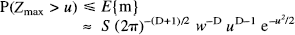
The probability of getting at least one voxel with a Z value of, say, height u or more, in a given SPM{Z} of volume S is the same as the probability that the largest Z value in the entire volume is greater than u. It can be shown (see Adler, 1981):

$\begin{array}{lll}{\mathrm{P}(\mathrm{Z}}_{\text{max}}>u)\hfill & ⩽\hfill & E\left\{\mathrm{m}\right\}\hfill \\ \hfill & \approx \hfill & S{(2\pi )}^{-(\mathrm{D}+1)/2}{w}^{-\mathrm{D}}{u}^{\mathrm{D}-1}\hspace{0.17em}{\mathrm{e}}^{-{\mathrm{u}}^2/2}\hfill \end{array}$

(13)

where E{m} is the expected number of maxima; wis a measure of smoothness and is related to the full width at half maximum (FWHM) of the SPM's resolution. In practice, w can be determined directly from the effective FWHM if it is known when w = FWHM/√(4log_e2) or estimated post hoc using the measured variance of the SPM's first partial derivatives. See Friston et al. (1991) and Worsley et al. (1992) for more details.

The p value based on n, the size of the region

The probability of getting one or more regions of, say, size k or more in a given SPM{Z} of volume S, thresholded at u, is the same as the probability that the largest region consists of k or more voxels P(n_max > k) where:

$\mathrm{P}(n_{max}⩾k)=1-exp(-E\{\mathrm{m}\}\cdot {\mathrm{e}}^{-\beta {\mathrm{k}}^{2/\mathrm{D}}})$

and

$\beta ={[\Gamma (\mathrm{D}/2+1)\cdot E\{\mathrm{m}\}/S\cdot \Phi (-u)]}^{2/\mathrm{D}}$

(14)

Φ(–u) is the error function (integral of the unit Gaussian distribution) evaluated at the threshold chosen (u). Eq. 14 gives an estimate of the probability of finding at least one region with k or more voxels in a SPM{Z}. In this paper, we present p values that are based on both the spatial extent and on peak height. The uncorrected p values are simply Φ(–u).

VALIDATION OF THE MODEL

We addressed the validity of the above model in three ways; (1) by examining the parameter estimates for biological plausibility using real data, (2) by examining the assumption of identically and independently distributed error terms using real data, and (3) by examining the distribution of the SPM values under the null hypothesis. To obtain data under the null hypothesis, we used a standard ¹¹C-Flumazenil binding study with no activation.

Data acquisition and experimental design

The data were obtained from a normal male subject in a manner approved by the local ethics committee and the Administration of Radioactive Substances Advisory Committee (UK). A radial arterial catheter was inserted with the subject under local anesthetic (bupivicaine 5%) into the nondominant arm and an i.v. cannula into the contralateral arm. Scans were obtained with a Siemens-CTI PET camera (model 953B CTI Knoxville, TN, U.S.A.) with performance characteristics as described by Spinks et al. (1992) and measured attenuation correction. ¹¹C-Flumazenil was prepared by a modification of the method of Maziere et al. (1984) and administered intravenously. About 6.7 mCi of activity was injected (248 MBq). Twenty-five emission scans were then collected. The duration of these frames ranged from 60 s in the initial scans to 900 s (3 × 1 min, 18 × 3 min and 3 × 15 min; in this particular study, the last frame was lost). Whole-blood radioactivity concentrations were monitored continuously with a bismuth germanate system connected to the arterial line. Discrete arterial samples were used to transform the whole-blood curve into a metabolite corrected well count calibrated plasma curve as described previously (Lammertsma et al., 1991).

Data preprocessing

The data were realigned and spatially normalised (Friston et al., 1995) (voxel size = 2 × 2 × 4 mm). The normalisation used a 12-parameter affine transformation that best matched the sum of all 25 frames to an appropriate template or model ¹¹C-Flumazenil image. This ¹¹C-Flumazenil template was taken from the SPM library of normalised images and was created by applying a nonlinear spatial normalisation (Friston et al., 1995) to an arbitrary normal ¹¹C-Flumazenil image (integrated over all frames) such that it conformed to the existing rCBF template. This normalising transformation solves simultaneously for a spatial and intensity transformation and accommodates differences in the regional distribution of tracers employed. Following normalisation the image was flipped and added to the un-flipped image and smoothed with a (8 mm FWHM) Gaussian kernel to provide a symmetrical ¹¹C-Flumazenil reference or template that conformed to the standard anatomical space (Talairach and Tournoux, 1988). Figure 3 shows the correspondence between the normalised integrated data (upper images) and the template (lower images). The data were then smoothed with an isotropic Gaussian kernel (FWHM of 8 mm). Only voxels exceeding 0.8 of the global activity for each frame separately were subject to further analysis. This is a standard threshold in SPM and selects voxels that are, predominantly, in gray matter.

FIG. 3.

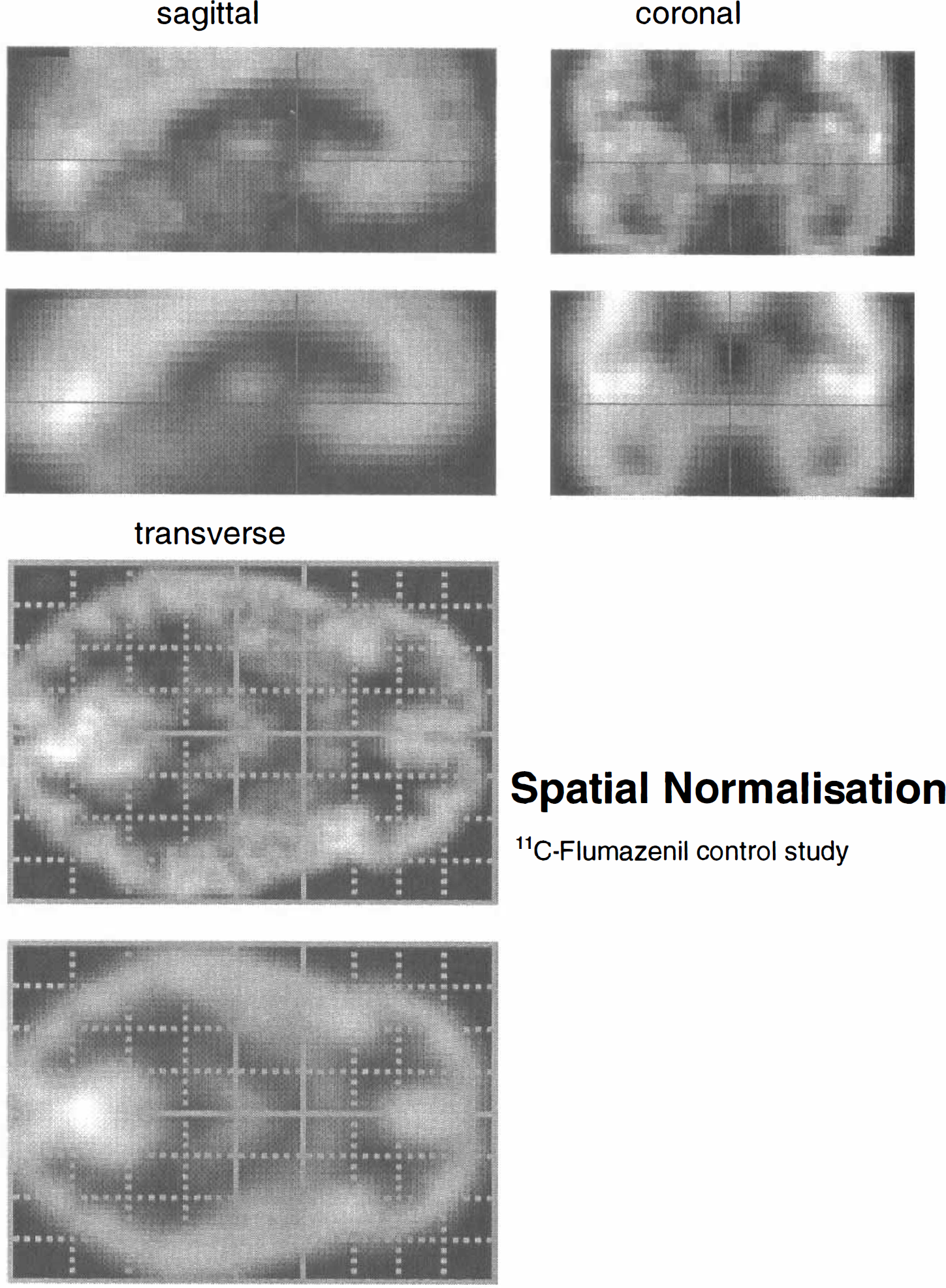
Orthogonal sections through the ¹¹C-Flumazenil data (integrated over all 25 frames), upper set, and corresponding sections through a Flumazenil template image; lower set, used in spatial normalisation. These sections are through the anterior commissure [0,0,0] mm following spatial normalisation. These data demonstrate the efficacy and quality of the spatial normalisation procedure. The normalisation used a 12-parameter affine transformation as described in Friston et al. (1995).

Statistical analysis

The whole blood and metabolite corrected plasma activity curves C_b and C_p are depicted in Fig. 1 (upper panel). The response variables and design matrices were computed as described in the theory section using the following values: κ₁* = 0.0077/s, κ₂* = 0.0045/s, δ* = 16 s, V_b = 0.1, and λ = 0.0056/s, the same values used in Figs. 1 and 2. The form of h(t) used in the current analysis is seen in Fig. 2 (broken line). The analysis provided estimates of relevant parameters and t statistics. The SPM{t} was transformed to a SPM{Z} and the distribution of Z values evaluated. The first frame was added to the second to reduce sensitivity to delay and dispersion of the estimated input function.

Parameter estimates

Values for k₂(0) _i and V_d(0) _i were estimated using Eqs. 8 and 9 for all voxels. The k₂ estimates were converted to the corresponding half-life ln2/k₂. Maximum intensity projections were then constructed for ln2/k₂(0) _i and V_d(0) _i . Figure 4 (upper panel) shows the spatial distribution of ln2/k₂(0) _i. It can be seen that the half-life of ¹¹C-Flumazenil is fairly uniform within cerebral gray matter, but there are some interesting regional variations: the ventral aspects of the temporal cortex, from extrastriate to inferotemporal and temporopolar regions have relatively high values of ln2/k₂(0) _i. The highest values are seen in the left medial temporal lobes. The distribution of this parameter (Fig. 4, lower panel) shows the estimates to centre on 700 s, in good agreement with previous estimates of the half-life for Flumazenil of about 12 min (720 s) in gray matter. The equivalent results for V_d(0) _i are shown in Fig. 5. In this instance, the greatest values are seen in the occipital and posterior cingulate cortices in accord with the distribution of receptor density and binding potential. The highest values are in the striate cortex and are about 5. This value is slightly lower than would be expected using more conventional analyses (a value of about 7 is typical). This disparity is probably due to the fact that the data have been smoothed and the regional values contain both gray and white matter contributions.

FIG. 4.

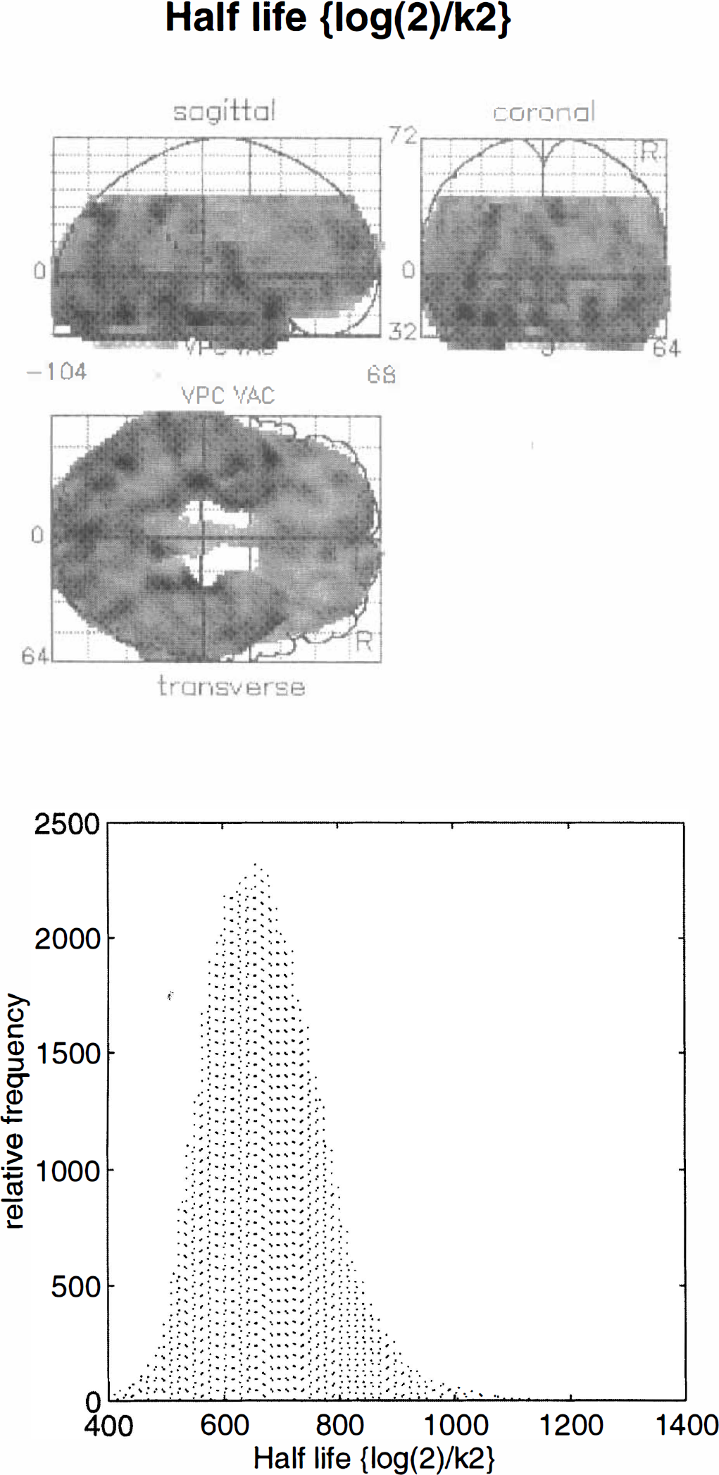
Upper panel: Maximum intensity projection of the initial half-life associated with k₂, estimated as described in the text for the validation study. The display format is standard and provides three views of the brain from the front, back, and right-hand side. The gray scale is arbitrary, and the space conforms to that described in the atlas of Talairach and Tournoux (1988). Lower panel: Histogram of the relative frequency distribution of voxel values displayed in the upper panel.

FIG. 5.

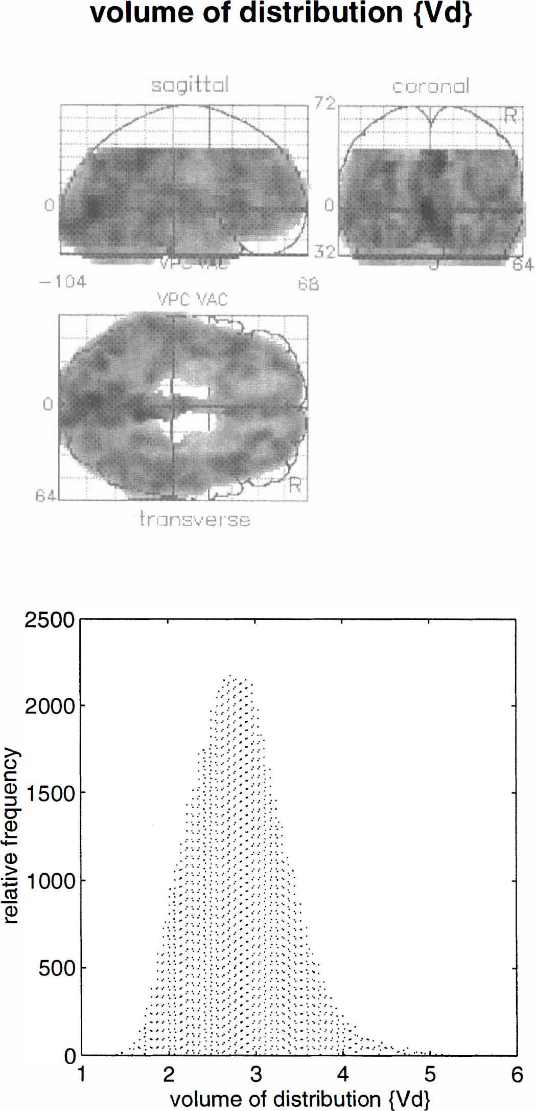
Upper panel: Maximum intensity projection of the initial volume of distribution V_d(0) _i estimated as described in the text for the validation study. The format is the same as in the previous figure. Lower panel: Histogram of the relative frequency distribution of voxel values displayed in the upper panel.

In summary, the estimates appear to have some validity in terms of both the quantitative and anatomical distribution. This validity, however, does not imply that the model is statistically valid. To be confident that the model is appropriate for making statistical inferences, we must demonstrate that the statistics obtained have the expected distribution under the null hypothesis.

Identically and independently distributed error terms

Identically distributed error terms implies homoscedasticity. Homoscedasticity refers to the homogeneity of error variances over observations (i.e., frames) and is an assumption that should be verified given the Poisson nature of the underlying data. Clearly, we cannot estimate the error variance for each voxel in every scan (there is only one observation per voxel per scan); however, we can partially validate the assumption of homoscedasticity by showing that the variance in the error term over voxels is roughly constant over frames. The sums of squares resulting from error were calculated according to Eq. 12 and plotted as standard deviations for each of the frames analysed. The results (Fig. 6) demonstrate that, with the exception of the first frame, the error terms are reasonably well behaved (homoscedastic). The independence of the error terms in Eq. 1 is guaranteed because they come from different time frames.

FIG. 6.

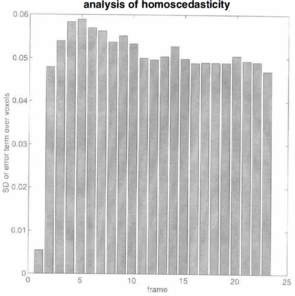
Standard deviation of the error terms estimated over all voxels analysed in the validation study plotted as a function of frame number. Ideally, they should all be the same.

Distribution of the SPM{Z} values under the null hypothesis

The distribution of the Z values for all the voxels analysed is shown in Fig. 7. The histogram details the empirically derived distribution, and the solid line is that expected under the null hypothesis; there is a reasonable agreement. It is also evident that there is a slight but definite bias toward negative values. The reasons for this may include (1) forcing multicompartment kinetics into a single compartment model, (2) real decreases in κ₂ during the latter half of the study, or (3) the effect of smoothing. This last possibility is suggested by the observation that the identical analysis of “unsmoothed” data removed this bias (results not shown). It is possible that smoothing confounds tissue compartments with different values for κ₂ and other parameters. This would “smear” the true spectrum of parameters and render a single compartment (mono-exponential) model more approximate. If this is the case, it suggests some interesting extensions of the approach considered in this paper; however, it should be noted that although the distribution in Fig. 7 is less than perfect, the bias is in the conservative direction for detecting increases in κ₂.

FIG. 7.

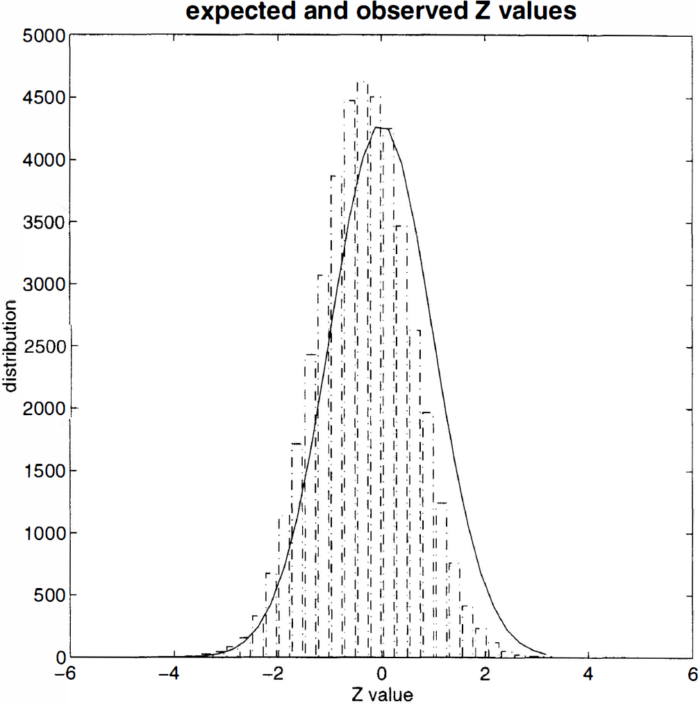
Expected and observed distribution of Z values from the validation study SPM{Z}.

A DYNAMIC DISPLACEMENT STUDY WITH ¹¹C-FLUMAZENIL

Study design and data acquisition

The data were obtained from a normal male volunteer and analysed in exactly the same way as in the previous sections. In this study, however, 50 μg/kg of midazolam was administered intravenously over 5 min between 30 and 35 min after beginning the study. The form chosen for the time-dependent change in κ₂[h(t)] was the same as that used in previous sections (the broken line in Fig. 2).

Parameter estimates

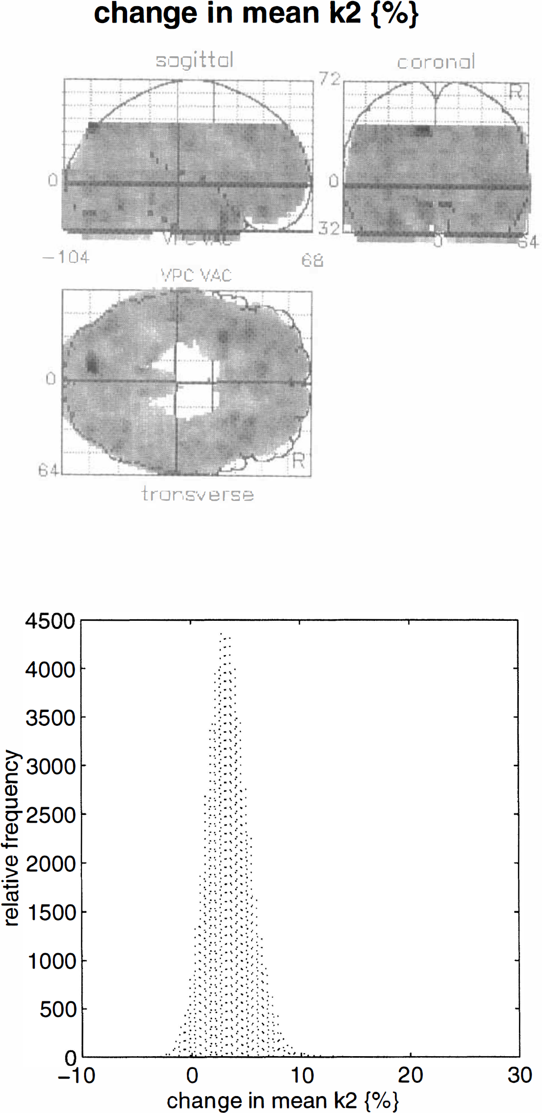
The parameter of interest in this study is g_i, the coefficient scaling the time-dependent displacement described by h(t). The maximum intensity projection of relative changes in k₂, calculated according to Eq. 10, is presented in Fig. 8 (upper panel). The corresponding distribution of relative changes (expressed as % change) shows these values to be largely positive with a maximum change of about 16%. These results pertain to the size of the effect but do not show whether these regional effects are significant or not. To make statistical inferences, one uses the corresponding SPM{Z}.

FIG. 8.

Upper panel: Maximum intensity projection of the average change in κ₂ estimated for the activation study. The display format is the same as in previous figures. Lower panel: The relative distribution of voxel values displayed in the upper panel.

Statistical inference

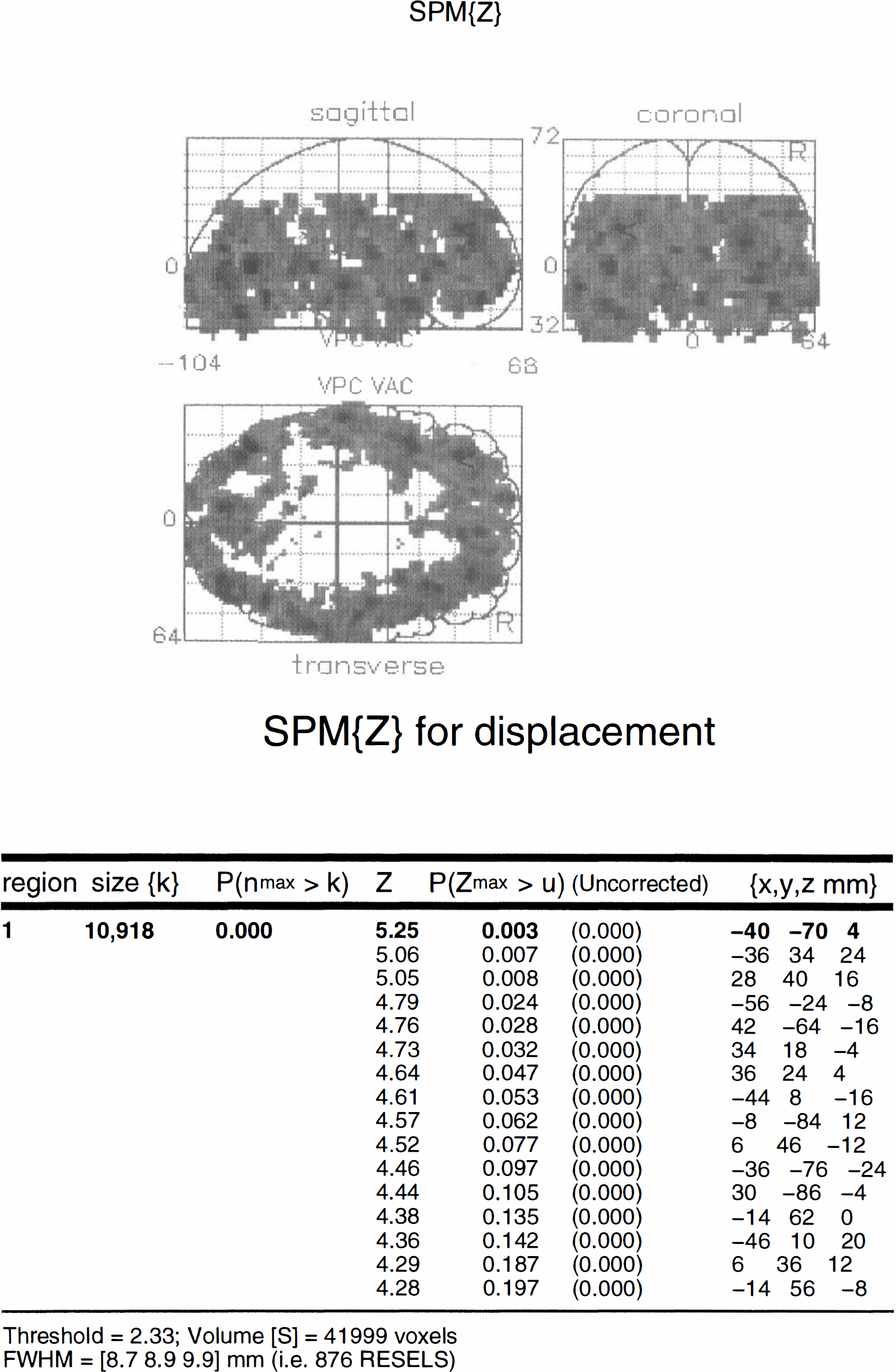
The SPM{Z} is depicted in Fig. 9. There was a remarkably significant effect (p < 0.01 uncorrected) in nearly all cerebral cortical gray matter regions. The highest Z score reached 5.25 in the left inferior occipitotemporal region. The next two most significant displacement effects were seen bilaterally in the left (Z = 5.06 p = 0.007 corrected using Eq. 13) and right (Z = 5.05 p = 0.008 corrected using Eq. 13) dorsolateral prefrontal cortices (DLPFC). The FWHM of the SPM{Z} were estimated to be 8.7, 8.9, and 9.9 mm in x, y, and z respectively. A total of 41,999 voxels were analysed.

FIG. 9.

Upper panel: Statistical parametric map SPM{Z}. This is a maximum intensity projection of the SPM{f} following transformation to the Z score. This SPM assesses the significance of the effects seen in the previous figure (Fig. 8). Lower panel: Tabular data are presented on regional effects in the upper panel. The locations of maxima within the largest region (10,918 voxels) are shown. For each maxima (Z), the significance is assessed in terms of P(Z_max > u) using Eq. 13 and its coordinates are provided.

The tissue curves for a voxel in the left dorsolateral prefrontal cortex or DLPFC (–36, 34, 24 mm) are shown in Fig. 10 superimposed on the curves predicted by the parameter estimates (solid line). The dotted line indicates what would have happened in the absence of any displacement. For comparison, the data for the same voxel from the validation study are shown in Fig. 11.

FIG. 10.

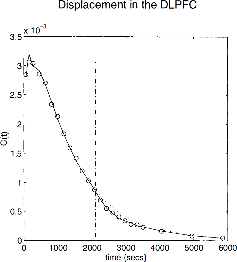
The observed (circles) and predicted activity (solid line) for a voxel in the left prefrontal cortex [–36, 34, 24 mm]. By omitting the component due to time-dependent changes, we can estimate the predicted activity in the absence of any dynamic changes in displacement (dotted line). The vertical broken line corresponds to the end of the midazolam injection.

FIG. 11.

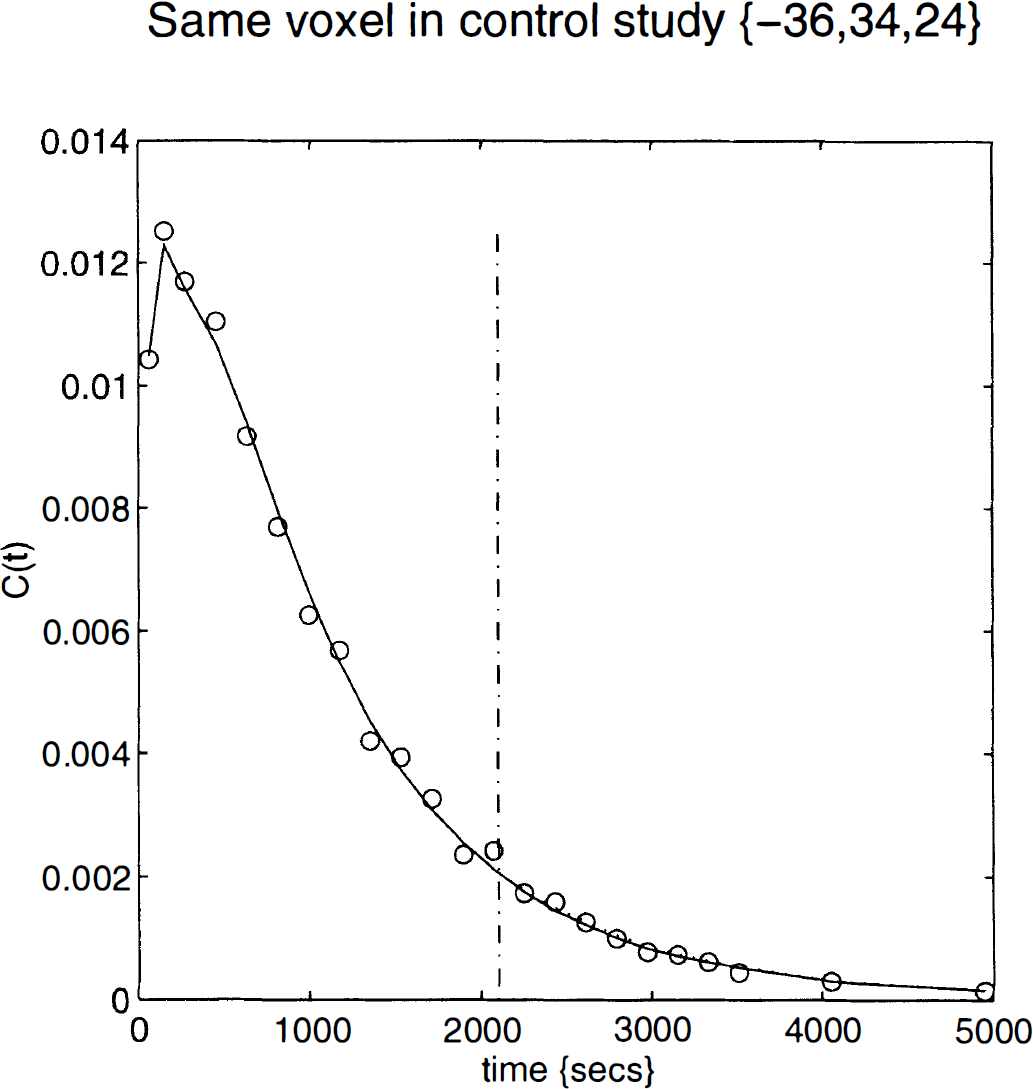
As for the previous figure (Fig. 10), but using data from the validation study.

Figure 12 shows the SPM[Z} rendered onto the Flumazenil template in three orthogonal sections through this DLPFC voxel. The bilateral involvement of the DLPFC, temporopolar regions, and extrastriate regions is evident in these sections and highlights some of the regional specificity and symmetry of the more significant effects.

FIG. 12.

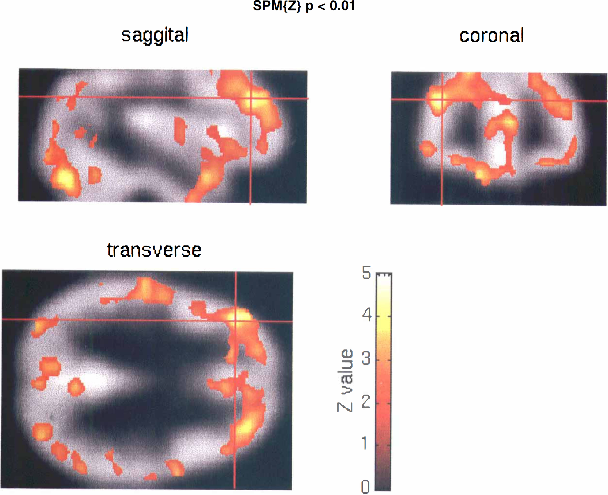
Orthogonal sections through the Flumazenil template (gray) with the statistical parametric map SPM{Z} (colour) rendered on top. The sections are through the voxel whose activity is depicted in the previous two figures. The SPM{Z} has been thresholded at p = 0.01 (uncorrected).

DISCUSSION

We have presented a simple way to detect the dynamic or time-dependent changes in displacement during single-subject radioligand PET studies. We hope the approach will facilitate dynamic activation studies using selective ligands. These studies are, in principle, capable of characterising functional neurochemistry in parallel with the use of rCBF activation studies to characterise functional neuroanatomy.

The proposed approach is based on union of a linear pharmacokinetic model and statistical parametric mapping and provides for a voxel-based assessment of significant regional effects. The statistical model used in this paper is predicated on a single-compartment model, extended to allow for time-dependent changes in specific rate variables. We have addressed the sensitivity and specificity of the analysis, as it would be used operationally, by applying the analysis to ¹¹-Flumazenil studies with and without a pharmacological challenge. We were able to demonstrate, and make statistical inferences about, significant increases in clearance (or decreases in the volume of distribution) in the prefrontal and other cortical areas. These changes might be attributable to the pharmacological effects of the midazolam challenge expressed at the level of central benzodiazepine receptors or via some other mechanism.

Limitations

The key limitation of the method described in this paper relates to the constraints and validity of the statistical model used. One key aspect of this model is that it has very few parameters (meaning many more degrees of freedom remain for statistical inference) and that it uses linear approximations. These linear approximations will fail if the observed kinetics deviate substantially from the canonical forms assumed for the tracer. This is a relatively safe limitation in the sense that a failure to model the real kinetics also implies a failure to model changes. This dual failure protects against false positives in regions where the model is inappropriate: the statistical model can be thought of as “focusing” on gray matter because the canonical curves assumed are typical of gray matter. This is an intuitive conjecture that will require a more formal analysis but, based on anecdotal observations, the conjecture seems reasonable.

A second limitation of the approach described here relates again to the validity of the model employed. In particular, a poor model may lead to bias. For example, the bias in Z scores observed in the validation study probably reflects the failure of a single-compartment model to fit the data properly from multicompartmental kinetics (either real or apparent, secondary to smoothing). Other explanations for this failure may include errors in the input function or potential interactions of the challenge with arterial measures. Many of these concerns would be addressed by using more elaborate kinetic models or by using spectral analysis to identify the number of compartments required. These and other ideas are the subject of current work (Vin Cunningham and Roger Gunn, personal communication).

Another limitation is that the form of the dynamic displacement changes is fixed and specified at the outset, thus precluding the possibility of regionally specific differences in the form of time-dependent displacement (e.g., phasic vs. sustained). This limitation and others are addressed in the next section on possible extensions of the current approach.

We have not presented any discussion on the timing of the acquisition frames in relation to optimising sensitivity to changes. Clearly, the challenge should be sufficiently late to render the evoked changes in kinetics relatively distinct from the kinetics themselves and yet not be so late that the changes occur in frames with poor counts. We do not address this issue here but acknowledge its importance for future work (see also Morris et al., 1995).

In this paper, we have focused on some of the methodological issues that arise in dynamic displacement studies. We acknowledge that many other pharmacokinetic issues will need to be addressed in the application of these sorts of techniques: For example, we have assumed that the changes in tracer clearance are due to interactions at the level of the receptor; however, other mechanisms may also contribute to the observed changes (e.g., changes in plasma protein binding of the tracer, peripheral metabolism of the tracer, tracer delivery, or changes in nonspecific binding).

Multicompartment models and complicated forms of time-dependent changes

In principle, the mathematical development described in the theory section can be extended easily to multicompartment models as described in the general approach section. Similarly, the expansion of the time-dependent effect on kinetic parameters [Γ _i (t)] can be in terms of many basis functions (e.g., polynomial, Fourier, and others), which would provide for a greater flexibility in the sense that maintained, phasic, or even biphasic time-dependent changes in displacement could be modelled. In this instance, the F ratio would be used to infer that some linear combination of the basis functions was sufficient to reduce the error variance significantly and the t statistic to test for specific linear combinations of these effects using a contrast with zero mean. Although we will be evaluating these extensions, it should be noted that the “minimal” analysis described above could be repeated for different forms of time-dependent changes in displacement [i.e., the shape of h(t) in Fig. 2 (broken line) could be changed to test for a more acute or even biphasic effect], resulting in a series of SPM{Z}, each testing a specific hypothesis about the form of dynamic displacement. Given that this facility exists, the usefulness of less constrained (and possibly less powerful) statistical models requires careful evaluation.

CONCLUSION

This demonstration study and methodological analysis point to the feasibility of dynamic displacement studies and appropriate statistical analysis. The experimental design and mathematical models used here are very simple, and yet the results obtained are compelling. This suggests a potential for the refinement of the proposed analysis and exploration of other approaches that could provide richer and more specific information.