
Abstract
Tests comparing image sets can play a critical role in PET research, providing a yes-no answer to the question “Are two image sets different?” The statistical goal is to determine how often observed differences would occur by chance alone. We examined randomization methods to provide several omnibus test for PET images and compared these tests with two currently used methods. In the first series of analyses, normally distributed image data were simulated fulfilling the requirements of standard statistical tests. These analyses generated power estimates and compared the various test statistics under optimal conditions. Varying whether the standard deviations were local or pooled estimates provided an assessment of a distinguishing feature between the SPM and Montreal methods. In a second series of analyses, we more closely simulated current PET acquisition and analysis techniques. Finally, PET images from normal subjects were used as an example of randomization. Randomization proved to be a highly flexible and powerful statistical procedure. Furthermore, the randomization test does not require extensive and unrealistic statistical assumptions made by standard procedures currently in use.
Tests comparing image sets can play a critical role in PET research. These tests provide a simple yes or no answer to the question “Are two image sets different?” before more qualitative or quantitative questions are asked about where the differences lie within the images. Sometimes an omnibus test provides a trivial answer to an obvious question: for instance, judging whether there is any difference in regional cerebral blood flow (rCBF) between two different cognitive task (A and B) conditions. In this case the omnibus test might reject the null or no-difference hypothesis, which absurdly conjectures that brain metabolism does not depend on cognition, and the test may be only ceremonial. On the other hand, an omnibus test sometimes provides important information. For example, a straightforward contrast might be germane when comparing images from two different language reading conditions in bilingual subjects.
An omnibus test to compare position emission tomography (PET) images is based on the notion of a significance test. The significance test has a specific and fundamental meaning in statistics: measuring the probability that an observed result could have occurred by chance. For instance, a frequently asked question is whether the differences between two sets of images suggest a significant change. Task B might be a memory task using a 5-s retention interval while task A uses a 60-s retention interval involving recognizing a word from a previously memorized list. Suppose that the area with the largest difference is 10% higher during task B in the left frontal region. The question arises as to whether this observed difference could have occurred by chance. Conceivably, there could be no real activation effect at all, yet random fluctuations could still produce 10% differences in various brain regions. If this chance probability is relatively high, say 5 in 10, then the 10% difference does not provide convincing evidence for an activation effect. On the other hand, if the chance probability is relatively low (e.g., less than 1 in 20), then the difference is typically interpreted as statistically significant using the conventional 0.05 type I error rate (alpha).
The statistical approach with this process is to determine how often such differences would occur by chance alone in repeated trials of the same experiment. An impracticable solution is to replicate the experiment many times using different subjects and randomly flipping whether a subject's A image was subtracted from B or vice versa. After a large number of replications, the number of comparisons that yielded differences as large as the original baseline activation difference would provide an indication of how unusual it would be for the observed 10% change in rCBF (from the previous example) to occur when chance alone is operating. The number of trials in which a difference of 10% or larger is noted divided by the number of repeated trials provides the probability estimate.
Another replication strategy, randomization or permutation, uses only the data from the original experiment. The notion that chance alone produced the observed difference implies that the task A and B images are interchangeable and that the observed difference is the result of a not-so-unlikely arbitrary arrangement. Instead of replicating the experiment de novo, a random switching of the condition labels would serve the same purpose. For example, Table 1 shows the possible arrangements of a study with three subjects. While subjects always retain their own data sets, the two voxel arrays would be arbitrarily reassigned to A and B producing a new pattern of A–B arrangements for each replication. The number of times that the difference from the original experiment occurs by chance can be readily ascertained by reference to the distribution generated from the replications.
Eight A-B B-A permuted samples generated by three subjects with paired image data sets
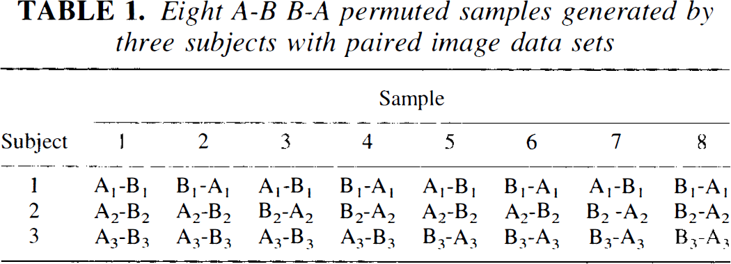
For small samples all possible (2 n ) arrangements provide the exact frequencies by enumerating all possible experimental results. For larger samples, a very large subsample of the permuted arrangements (e.g., 5,000) provides an accurate approximation. These tests are variously and sometimes interchangeably referred to as randomization, permutation tests, or Monte Carlo tests. A number of authors have expressed a preference for these types of tests since they are applicable to any population and do not explicitly assume random subject selection (Fisher, 1936, 1990; Pitman, 1937a,b, 1938; Edgington, 1966, 1995), although generalizations from any theoretical or randomization test on a particular sample may be constrained to the sampling procedure.
There are several advantages to using randomization to obtain probabilities. These estimates are based on an empirical definition of probability. Randomization methods produce results that make no assumptions about the nature of the data distribution since no reference is made to a theoretical curve or function. The process is also extremely flexible. Tests of mean differences, correlations, and differences in correlations can be produced for the whole brain (an omnibus test), sets of regions of interest (ROIs), or individual voxel areas. The only requirements for a test are that a single-valued test statistic (e.g., a single summary value characterizing the effect of interest) can be found and that the sample is large enough to randomize. This sample size requirement is actually very liberal since as few as 10 subjects in an A-B condition experiment will produce (210 =) 1,024 permutations.
PET and other imaging research created new statistical problems for which standard tests often do not adequately apply. Important pioneering work has been done by Worsley et al. (1992) and Friston et al. (1991) to modify and extend simple statistics to an omnibus test for PET applications. Both groups have derived theoretical probability distributions for a test of PET images.
The techniques of Worsley et al. (the Montreal method) and Friston et al. (SPM94) have been compared by Arndt et al. (1995). Both begin with an omnibus test for the sets of images being compared and both calculate a t test for each voxel location in the data set. The highest t value (tmax) is used as the criterion for determining whether the image sets differ in this initial omnibus test. Both can represent the voxel comparisons with a t image. A distinction between these two methods is how they estimate the standard deviation (SD) used for calculating the t values. The Worsley method uses a single SD found by pooling the SDs from all voxels. SPM uses the local voxel SD. Both of these methods attempt to account for the number of tests performed, by reference to the theory of Gaussian random fields (Adler and Hasofer, 1976; Hasofer, 1978). Randomization tests of tmax have also been suggested in the statistical literature (Chung and Fraser, 1958; Boyett and Shuster, 1977) but only recently applied to imaging data (Holmes et al., 1996).
Test statistics other than tmax may be more powerful or more interesting to the PET researcher. In questions about whether two sets of images differ, a general test that makes use of more information than the tmax has been advanced by a number of authors (Chung and Fraser, 1958; Blair and Karniski, 1994; Good, 1994; Edgington, 1995; Worsley et al., 1995). This test is based on the sum of the image t2s (Σt2), which may be more sensitive to moderate changes or differences that may involve several peaks or a large flat region of activation. Unlike the tmax statistic, Σt2 is a composite of all image t values.
Whatever the potential advantages of Σt2 or other multivariate tests, their application to imaging data has been hampered since the standard reference distribution (Hotelling's T2 or the multivariate F) is not applicable. Imaging data often do not meet the necessary assumptions, and multivariate analyses typically require more subjects than voxels. Worsley et al. (1995) have recently outlined a solution to the distribution of Σt2 using the theory of Gaussian random fields. However, randomization methods are appropriate. Manly (1991) also describes several other statistics that may be applicable.
The present paper examines the use of randomization methods to provide omnibus tests for PET images. In the first series of analyses, normally distributed image data are simulated that fulfill the requirements of standard statistical tests and present a simplest case scenario. These analyses were used to generate detection rates and to compare the tmax and Σt2 statistics under optimal conditions. Varying whether the standard deviations were local or pooled estimates provides an assessment of a distinguishing feature between the SPM and Worsley methods. In a second series of analyses, we more closely simulate current PET acquisition and analysis techniques by examining data that have been smoothed with a filter. Finally, PET images from normal subjects are used as an example of this technique.
MATERIALS AND METHODS
Analysis 1: Simulation using white noise data with peaks inserted
The first set of analyses were conducted on white noise images generated using normally distributed independent voxel elements. All calculations were performed on a Macintosh Power PC 7100 in MATLAB (Mathworks, 1995). The random numbers were produced by the algorithms given in Forsythe et al. (1977). A test of this generator with 5,000 random numbers showed no significant spatial dependence (inter pixel r = 0.003, 95% confidence interval: −0.0247 ≦ p ≦ 0.0308).
For the number of randomizations, we chose 5,000 replications when the full set of permutations became impractical. This was a compromise between practicality and attempting to obtain accurate estimates of p values near the critical p values used in hypothesis testing. Using a variety of methods, Manly (1991) calculates the 99% confidence intervals around the p < 0.05 cutoff obtained with 5,000 replications to be 0.042–0.058. Using central distribution free intervals (Stuart and Ord, 1987, formula 20.131), we found the same values for the 99% interval and between 0.056 and 0.044 for the 95% confidence interval. Around the 0.01 probability estimate, 5,000 replications provided a confidence interval of approximately ± 0.003.
For each analysis, n (= 10, 15, 20, or 30) A–B image pairs were constructed with 512 elements. To find the critical values, the image pairs were either fully permuted (n = 10) or randomly reassigned 5,000 times to different A–B combinations. Thus, for each subject's pair of images, the arrangement A minus B or B minus A was randomized for the replication. After each rearrangement, the image sets were averaged and an SD was found for each pixel location (local SD). The pooled SD was also calculated. These values were used to generate two images made from the local or pooled pixel-based t tests. Thus, each t image was based on 512 t tests. The largest absolute t value from the local and pooled t images, local tmax and pooled tmax, as well as the sum of local and pooled t2 (i.e., Σt2) were stored after each resampling. After all replications, the resampled statistics were sorted, and the value cutting off the most extreme 5, 2.5, and 1% of the distribution were used as the alpha level p < 0.05, 0.025, and 0.01 critical values. Although this procedure was instructive, other algorithms, such as described in analysis 2 below, are more efficient for real applications.
Detection rates were calculated in a similar fashion. Before rerandomizing the image pairs, an effect (δ) was added to an image location. The effect sizes (ES) were equal to δ divided by the local SD, thus an ES = 1 added 1 SD to form the peak. The effect was added to the same randomly located voxel in all n images. Effect sizes of 0, 0.5, 1, and 2 were added. The effect size denoted as [1 1] placed two peaks in the image. Other effect size conditions involving multiple peaks were also investigated. The test's detection rate was defined using the number of replications that produced statistics exceeding the critical values chosen for this simulation experiment (e.g., the frequency that the image would have been significant). The number of significant (i.e., observed tmax > critical value) replications was divided by the total number of replications to form approximate detection rates.
Critical values and power estimates were also found for the methods of Worsley et al. (1992) and the SPM94 program, using pooled and local SD tmax values, respectively. A three-dimensional random field made from 512 independent normally distributed numbers [i.e., N(0,1)] contains approximately 314 resels (resolution elements) in the 512 images based on formulas in Worsley et al. (1992). Formula 1 in Worsley et al. (1992) provided critical values corresponding to standard p values (i.e., 0.05, 0.025, and 0.01). The critical values for SPM were found using the SPM program (subroutine SPM_PZ.M in SPM94) using formulae discussed by Friston et al. (1991, 1995). To find the smoothness parameters (Friston et al., 1991) for our random images, we passed SPM94 10 pairs of images containing 46,256 independent random numbers. This produced the three smoothness parameters 1, 1, and 0.5. These smoothness values, the image, and the sample size were used to generate the critical values for our images. Once a critical value was established, we noted the number of times each method signaled a significant value; the number of times the observed tmax exceeded the critical value divided by the number of replications was the detection rate.
Analysis 2: Using a lifelike phantom
In the second set of analyses, a more lifelike phantom simulation was used with n = 20. These consisted of a 3D array of approximately 445,700 voxels for each “subject” and was valued using a normally distributed random number with constant mean and SD. After their initial generation, the 3D arrays were smoothed using a 18.33-mm Hanning filter resulting in approximately the same number of resels that we find in our center's PET experiments. Calculations were performed on a Silicon Graphics workstation (running IRIX version 5.3 and using a 150-MHz IP22 processor) and the randomization program was written in the C language. The random number generators were based on standard published algorithms (Griffiths and Hill, 1985; Press et al., 1992). Computational efficiency was increased by updating summary statistics rather than recalculating the sample statistics and sequencing the randomization samples to minimize the updating workload using published algorithms (Bitner et al., 1976; Lam and Sotchen, 1982). As in the prior analyses, the program computed both local and pooled forms of tmax and Σt2. Probability estimates were provided using randomization, the formalizations of Worsley, and the subroutine in SPM94. Visualization of the image was accomplished using BRAINS (Andreasen et al., 1993).
Analysis 3: Human PET data
Subjects. Subjects were 20 healthy normal volunteers recruited from the community by newspaper advertising. This sample is a random subset of data that has been previously published (Andreasen et al., 1995). Their demographic features have been previously described. All gave written informed consent to a protocol approved by the University of Iowa Human Subjects Institutional Review Board.
Memory tasks. The complete study in which these subjects participated was designed in order to explore aspects of recognition memory using variable retention intervals. A substudy on verbal memory included two retention intervals (short and long) plus a comparison condition (reading words); this study has been described in detail in a prior publication (Andreasen et al., 1995). For this analysis, we focus on the positive activations from one subtraction from this study: long-term memory for words minus reading words. For the experimental condition referred to as “long-term memory,” subjects were trained until they had perfect recognition memory of a group of 18 words during the week prior to the PET study; the group of words was again reviewed on the day before the PET experiment in order to ensure that it was still well learned. The comparison condition consisted of reading common English words. All words consisted of one- or two-syllable concrete nouns that were presented visually on a video monitor.
We used the same algorithms and C language program as in analysis 2 with the lifelike phantom to perform randomization tests on images from 20 subjects. The methods for PET and magnetic resonance (MR) data acquisition have been previously described (Haining, 1990; Hurtig et al., 1994; Andreasen et al., 1995). The PET data were acquired with a bolus of 75 mCi of [15O]H2O in 5–7 ml saline using a GE PC4096-plus 15-slice whole-body scanner. MR scans were obtained for each subject with a standard T1-weighted three-dimensional SPGR sequence on a 1.5-T GE Signa scanner (TE = 5, TR = 24, flip angle = 40, NEX = 2, FOV = 26, matrix = 256 × 192, slice thickness 1.5 mm). The anterior commissure–posterior commissure (AC-PC) line was identified and used to realign the MR image of all subjects to a standard position. The PET image for each individual was fit to that individual's MR scan using a surface fit algorithm (Levin et al., 1988; Cizadlo et al., 1994). The MR images from all subjects were averaged using a bounding box technique, so that the functional activity visualized by the PET studies could be localized on coregistered MR and PET images where the MR image represented the “average brain” of the subjects in this study (Andreasen et al., 1994, 1995). An 18.33-mm Hanning filter smoothed the PET images for each condition to eliminate residual anatomical variability. MR images were then aligned on the AC-PC axis and the interhemispheric fissure. Images were resampled to 128 × 128 × 80 voxels using the Talairach Atlas image space (Talairach and Tournoux, 1988). After thresholding the image to 150% of the mean voxel value to isolate brain, there were 522,141 voxels in the images.
RESULTS
Analysis 1
From a statistical perspective, maintaining a consistent known probability of mistakenly finding significance (the alpha level or type I error rate) is the primary constraint on a statistical test. Standard testing procedures use tabled functions to provide a critical value that, when exceeded, signals an unlikely and significant (p < alpha) event. For the following analyses, we chose the conventional alpha level of 0.05. However, the trends may be generalizable for any usual nominal alpha levels.
Critical values cutting off the most extreme test statistic corresponding to a p value < 0.05 were found empirically by randomizing simulated images. Results for both tmax and Σt2 statistics, calculated with pooled and local SDs are shown in Table 2 for samples of 10, 15, 20, and 30 subjects. These values were obtained by generating five different experiments at each sample size, randomizing them each, and then averaging. Table 2 also shows the corresponding values based on Gaussian random field theory using Worsley's method for the pooled SD tmax and SPM94 for the local SD tmax. The data were normally distributed and all generated with a common SD. Randomization of the larger sample size included 5,000 replications while the complete series of 210 (= 1,024) permutations was generated for the sample size of 10.
Critical values (p ≤ 0.05) produced by randomization a of normally distributed data for t max and Σt2 statistics in an image containing 512 independent elements
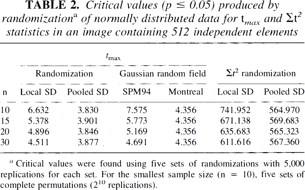
Critical values were found using five sets of randomizations with 5,000 replications for each set. For the smallest sample size (n = 10), five sets of complete permutations (210 replications).
The randomization tmax and Σt2 critical values based on the pooled SD were consistently smaller than those based on the local SD. The locally based values decrease as the sample size increases but are still considerably larger than the corresponding pooled values at n = 30. The increased values result from the added instability of variable local SD estimates producing a wider distribution. The instability in the SDs is particularly noticeable for small samples.
The tmax for a 0.05 significance threshold produced by SPM94 and the Worsley et al. (1992) formulations are also shown in Table 2. The tmax values for the 0.05 significance levels produced by SPM94 were consistently larger than the corresponding local tmax critical values found using randomization. At the largest sample size (n = 30), this difference became less pronounced, with SPM94 providing a critical value of 4.69 compared to the randomization value of 4.51. Similarly, the formula given in Worsley et al. (1992) produced values consistently larger than the corresponding critical values from randomization using the pooled SD. Since the pooled SD is based on a very large number of voxel locations and thus has an extremely large number of degrees of freedom, Worsley's formula does not depend on n and produces a value of 4.36 for all sample sizes. For these randomly drawn images, the SPM94 and Worsley methods were always conservative when no peak was present in the image.
We evaluated how often these values erroneously signal a significant difference in a repeated series of random images. Ideally, the α = 0.05 critical values should be exceeded less than 5% of the time in repeated samples or replications. The proportion of times that the repeated sample produced a “significant” value when there was no difference between the image sets (effect size = 0) is shown in Table 3. The critical values from randomization produced error rates that were all very close to the expected 0.05 level.
Detection rates for two randomizationa tests (t max and Σt2) using local and pooled standard deviations (SD) in a 512 independent element image of varying sample sizes (n) and peak effect sizes (ES)
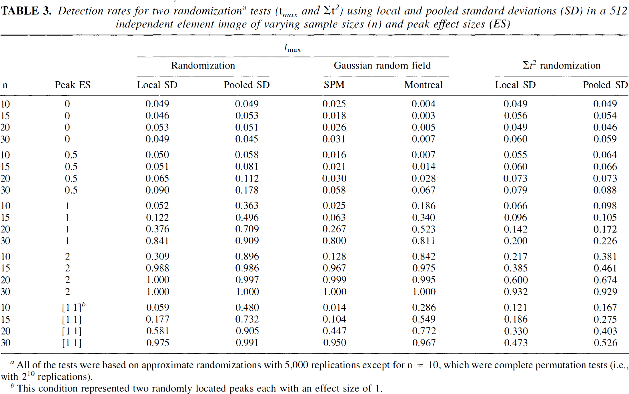
All of the tests were based on approximate randomizations with 5,000 replications except for n = 10, which were complete permutation tests (i.e., with 210 replications).
This condition represented two randomly located peaks each with an effect size of 1.
Detection rates for the tests in several different situations are also shown in Table 3. Peaks were manufactured by inserting a hot pixel in a second set of randomizations. The magnitude of these hot spots was indexed by the effect size (i.e., mean difference divided by the SD) (Cohen, 1988). The frequency that the modified images crossed the critical value was tabulated, and the proportion of times the test suggested a significant difference gives a rough indication of the test's power. Ideally, several thousand datasets, each randomized several thousand times, would be needed to provide power estimates. Since such an effort would be impractical, we chose to provide this more limited assessment of power referring to correct rejection of the null hypothesis as the detection rate.
In the presence of real peaks, the test statistics based on pooled SD estimates tended to find the significant results more often than the statistics using local SD estimates. For instance, when n = 20 and there was a significant peak with an effect size of 1, the pooled tmax found a significant (p < 0.05) result more than 70% of the time (detection rate = 0.709). However, using the local tmax statistic, significance was seen less than 40% (detection rate = 0.376) of the time. Thus, when the assumption of a constant SD holds, the pooled estimate is a better choice. For large samples (n = 30) and large effects size (≧ 1.0), both local and pooled tmax statistics produced excellent detection.
Interestingly, SPM94 and the Worsley method, despite their initial tendency to conservatism when no peaks were present, provide good power at the largest sample sizes for effect sizes ≧ 1. These methods were always somewhat less powerful than the randomization tests.
The Σt2 statistic had a lower detection rate than tmax for all of the effect sizes shown in Table 3. This test statistic seems to perform better when there are many peaks spread over a large area. For instance, when 2% of the image was covered (10 peaks in 512 elements) with a 0.5 effect size (n = 15), the local and pooled tmax statistics had detection rates of 0.07 and 0.31, respectively. The rate of the pooled Σt2 was higher, at 0.34. Thus, for multiple areas or a single diffuse area of low-level activation, the Σt2 statistic may be preferable to tmax.
Analysis 2
In this series of analyses, two different sets of images were produced: a null condition set with no differences between the A and B contrast and one with a fairly robust peak (effect size = 2) added. Each analysis used 20 image pairs smoothed with a 18.33-mm Hanning filter. As with the previous analyses, the data were normally distributed, had a constant SD throughout the images, and fulfilled the assumptions of a Gaussian random field.
As expected for the null condition comparison, none of the statistical tests suggested a significant difference in the A – B subtraction. The observed local SD tmax was 5.499, which was less than the p < 0.05 critical value of 6.38 based on randomization. The likelihood of finding a (local) tmax this large during the 5,000 replications was p < 0.216. Similarly, using the pooled SD, the 0.05 critical value of tmax was 5.28 and the observed value was 4.20. This was not an unusually large tmax, since nearly two thirds (63.38% or p < 0.634) of the random replications produced a value this large or larger. The Worsley et al. (1992) formulas and the pooled tmax gave a p value of 0.162, which was considerably smaller than the randomization p value, but larger than 0.05. SPM94 produced an omnibus p value of 0.216. Also, the Σt2 statistic yielded nonsignificant results with p values of 0.201 and 0.159, for local and pooled versions, respectively. Thus, none of the tests provided a false positive result.
In contrast, all of the omnibus statistical tests signaled a significant difference when the single peak was added. The local tmax was 9.46, located at the peak's location. A value of 6.42 or larger would have been significant at the α = 0.05 level. The actual p value from the randomization of local tmax was 0.004. The pooled SD version of this test gave similar results. The 0.05 critical value was 5.43, while the observed tmax was much larger, 8.07. The approximate p value was p < 0.0002. Both the local and pooled Σt2 statistics produced randomization p values of < 0.0004. The probabilities based on the randomization technique were very similar to those based on the Worsley (p < 0.0001) and SPM94 (p < 0.0003) methods.
Analysis 3
Comparing a real set of 20 PET image A – B pairs from normal subjects, all of the statistical procedures again agreed in assessing the probabilities. The pooled tmax was 7.44 for this image subtraction. Based on the randomization method and 5,000 replications, this tmax had a probability of 0.0024, while the method of Worsley provided a p value less than 0.0001. The local tmax was 8.56. According to the randomization distribution, this value had a probability of 0.0018, which was somewhat larger than the value offered by SPM, p < 0.0001. While the two theoretically based probabilities were considerably more liberal, all of the methods of testing tmax suggested a significant difference between the A – B image sets. Likewise, the two Σt2 statistical tests suggested highly significant differences. None of the 5,000 randomized images provided local or pooled Σt2 statistics that were larger than the observed. Hence both p values were less than 1/5,000 (= 0.0002).
DISCUSSION
Randomization tests offer advantages over standard tests that use approximate reference distributions. An important statistical advantage is the consistent protection against the nominal type I error rates or the frequency of mistaking a nonsignificant difference as significant. The randomization test always provides a close approximation to a 0.05 cutoff when the 0.05 critical value is chosen. The exact confidence intervals for this approximation can also be calculated (Stuart and Ord, 1987; Noreen, 1989), but typically these intervals are small enough to be inconsequential when a reasonable number of replications is used. In contrast, procedures that rely on distributional assumptions can be affected when their assumptions do not hold. Both SPM94 and the method detailed by Worsley et al. (1992) make extensive distributional and large sample assumptions about the data throughout their calculations. Some of these assumptions are outlined in Friston et al. (1991), Worsley et al. (1992), and Arndt et al. (1995) and include: the independence of mean and SD, an independent and identical distribution of the errors, and an isotropic spatial correlation (Upton and Fingleton, 1990; Cressie, 1993) over the entire image defined by first-order (i.e., next-pixel-over) correlations. While all of the testing procedures agreed somewhat on our lifelike phantom and actual PET images, they need not do so. In one analysis from an early small (n = 10) PET pilot project, the Worsley method of calculating an omnibus test provided a p < 0.0033. However, a complete permutation revealed that this tmax value occurred in almost 8% of the random arrangements. Either the application of Gaussian random field theory to this particular set of images was inappropriate or the number of resels was incorrectly estimated.
Both SPM and the Montreal method require an explicit estimate of the spatial dependency within the image. In SPM, this estimate is referred to as the image smoothness, and in the Worsley method the dependency underlies the notion of resel. These estimates of spatial dependence are based on first-order serial (i.e., next-pixel-over) correlations or are assumed to be a function of the spatial filter used during image processing. None of these estimation procedures considers that the brain is a highly integrated organ and naturally exhibits an orchestrated pattern of activation. To assume that the only correlations among brain voxels are caused by image filtering and can be estimated by next-pixel-over correlations ignores the biology and is likely an oversimplification. Randomization tests do not require these assumptions.
In addition to the flexibility afforded by few statistical assumptions, randomization tests have been suggested for different testing situations (e.g., tests of multiple groups), different statistical measures (e.g., Σt2, Pearson rraax, Σr2, Mantel's spatial correlation), and may be extended to other imaging modalities (e.g., single photon emission computed tomography, fMRI). For instance, analysis of fMRI often correlates an input (stimulus) wave form with voxel values over time resulting in a (Pearson or Spearman) correlation and a phase offset for each voxel (Bandettini et al., 1993). Either the image of correlations (r) or phase offsets (φ) may be of interest. Group comparisons of either r or φ can be easily tested with randomization. However, novel statistics should be adequately investigated before randomization, since new indices of an effect may react in unexpected ways.
The performance evaluation of the Σt2 statistic appears mixed. In the simulations, we created isolated peaks in the data set. The Σt2 maintained the nominal alpha level of the test (0.05), but was clearly less powerful than the tmax statistic. This was perhaps an unfair comparison of these two alternatives since the peaks were unrealistically focal. Most cognitive activations produce multiple areas of activation corresponding to the various structures called upon in the task. In the actual PET data (analysis 3), the Σt2 statistic clearly provided the strongest case for rejecting the notion that chance alone was responsible for the differences. None of the 5,000 random arrangements produced a Σt2 as large as the value observed when contrasting the two cognitive conditions placing the p value at something less than 1/5,000. Thus, as noted by Worsley et al. (1995), the Σt2 may be an extremely powerful alternative omnibus test statistic.
The power of randomization tests applied to real data is difficult to determine theoretically. However, asymptotically, a randomization procedure will have power rivaling the most powerful possible test (Manly, 1991; Good, 1994). For smaller samples, the randomization test may have less power than one based on Gaussian random field theory. This advantage usually exists only if the assumptions hold true and the estimates of smoothness or resel size using next-pixel-over correlations are correct. Based on experience in other situations (e.g., the Mann-Whitney and Wilcoxen tests), when the assumptions are violated, the randomization test is often more powerful, sometimes strikingly so. Violating the Gaussian or other assumptions of a theory-based test sometimes increases the alpha level above the nominal level. Thus, the tabled values of a standard test's 0.05 threshold become too liberal. Post hoc corrections of the theoretical significance threshold often make the theory-based test less powerful than the randomization alternative. On the other hand, randomization tests always hold the alpha level close to nominal level (e.g., 0.05). Moreover, the most powerful relevant test for an experiment will be one that best characterizes the effect of interest. As we have noted, randomization tests can be applicable to a variety of statistics.
After a significant omnibus test statistic, regional analyses are necessary to find out how and where the image sets differ. Unfortunately, there are no good exact solutions for this problem. Several papers (McCrory and Ford, 1991; Bandettini et al., 1993; Blair and Karniski, 1994; Holmes et al., 1996) have discussed a number of problems and possible solutions. Worsley et al. (1992) suggested using the critical value of tmax as a cutoff or threshold for the entire image of t values. The logic is that any excursion area that protrudes above the critical value threshold would have signaled a significant difference between the image sets. Thus, by implication, any excursion set of voxels can be said to be significant. Since this is similar to a Bonferroni correction for the number of resels, this is likely a conservative estimate. Other more powerful post hoc thresholds have been developed theoretically (Hochberg and Tamhane, 1987) and suggested by Blair and Karniski (1994). These step-down procedures check the largest t value in the image, then the second largest, and so on. With randomization, these techniques require regenerating a new randomized distribution at each step. Holmes et al. (1996) provide examples, discussion, and simple algorithms for these tests applied to PET data.
As we mentioned in the introduction, omnibus tests are sometimes very important. However, often an overly general test is of less interest than tests of local areas or structures. In some instances, the question, “Is there a difference somewhere?” is immaterial or even counterproductive. For instance, large interindividual differences coupled with the basic between-group similarity of cerebral blood flow may make it difficult to obtain a significant omnibus test when an actual group difference is restricted to a single small area. Specific regional (ROI) contrasts do not require an omnibus test if these contrasts were hypothesized a priori. However, when a number of a priori contrasts are made, appropriate adjustments are necessary. Standard procedures are available to adjust the alpha level of the test or the test can be randomized using either ROI-based tmax or Σt2. Exploratory analyses represent another situation where omnibus testing may be inappropriate. In this case, whether to use significance testing procedures at all during the exploratory phase could be arguable since other, more appropriate procedures may be available (e.g., effect size estimation) (Cohen, 1988; Andreasen et al., 1994).
One issue with any randomization method is that it is computation intensive. For many situations, efficient algorithms and fast computers make randomization an attractive solution. There may, however, be questions about how practical it might be for a given experimental design or for a sample size. We have found that simple two-condition contrasts even with large samples (n > 30) are acceptable, particularly if the number of replications (N) is reduced to 3,000. While with the more efficient algorithms, the number of replications does not linearly affect the amount of time required for a randomization, fewer replications do produce quicker solutions. However, reducing N affects the precision of the probability estimates. Fortunately, the precision of an estimated cutoff (e.g., 0.05) can be easily predetermined. This procedure and the formulae required are discussed in Manly (1991). Noreen (1989) provides tables and formulae for one-sided confidence intervals and Stuart and Ord (1987) provide the formulae for two-sided intervals. In general, if all that is required is a simple yes–no answer using a predetermined p value cutoff, fewer replications are necessary than if the actual goal is to provide an accurate estimate of the randomization probability.
The logic for randomization tests has been accepted in principle for over half a century. Fisher (1936) notes that reference to standard mathematical distributions for tests has no justification beyond its agreement with a simple randomization procedure. Many basic statistical tests are based squarely on permutation logic, for instance, Fisher's exact test (Fisher, 1990), tests of Spearman and Kendall correlations (Kendall and Gibbons, 1990), and Mann-Whitney, Wilcoxen, Kruskal-Wallis, Friedman, and Pitman tests (Pitman, 1931a,b, 1938; Conover, 1980). Fisher (1936) noted the main drawback for widespread use of randomization procedures: the required computations. The availability of fast computer chips has, to a great extent, removed this obstacle. Given their advantages, ease of interpretation, consistent protection against type I errors, the potential for increased power, flexible choice of the tested statistic (e.g., tmax, Σt2, Σr2), and the ability to use any imaging modality, randomization tests have clear advantages over other testing procedures.
Footnotes
Abbreviations used
Acknowledgment:
This research was supported in part by NIMH grants MH31593, MH40856, MHCRC 43271, MH00625, and an Established Investigator Award from NARSAD.