Coverage and Reliability of Randomly Distributed Sensor Systems with Heterogeneous Detection Range

Abstract

In this article, we examine the coverage and reliability of distributed sensor networks that are designed for surveillance applications. In particular, we examine a model of sensor network coverage based on Poisson processes, and illustrate how this model combines with standard reliability models to provide estimates of field degradation over time. The results of the article illustrate how the number of sensors required changes with respect to reliability criteria, and how to design and re-seed sensor fields to maintain a minimal level of surveillance coverage. The formulation in the article is presented analytically, and all results are compared to numerical simulations.

1. Introduction

Distributed sensor networks are rapidly becoming a ubiquitous component of modern surveillance systems. Recent advances in computing, manufacturing, wireless communications, and power electronics have made the deployment of many small autonomous sensors an affordable alternative to large manned sensing platforms [1–3]. The general goal in deploying a large surveillance sensor network is to detect and/or track a target that has entered the surveillance region. Examples of such networks can be found in [4] and [5]. A particular feature of the target surveillance application is the use of sensors in environments where communications are constrained, and where specific placement is limited to spreading sensors according to a prescribed sensor density. When communications are readily available, various sensor planning algorithms (such as [6]) are available to carefully query and allocate sensor resources. However, under the constraints of difficult environments (such as the undersea environment), the sensor field's performance is enhanced only through careful initial planning of sensor placements. With good performance models, the deploy-and-forget planning of sensor fields for desired performance is possible. Suitable performance models for this type of planning have been developed for the cases of random deployments [7], clustered deployments [8], and for heterogeneous mixtures of sensors [9].

The analysis of the target tracking performance of distributed sensor networks is much more complicated than simply determining the “packing coverage” for sensors placed on a rigid grid. In recent practice, models of random placements combined with idealized individual sensor performance models are often used to provide rough order-of-magnitude estimates for the performance of actual systems. These models are particularly good at capturing trends in performance characteristics relative to deployment density and sensor characterization; such results are crucial for applications where large deployments are rapidly made over potentially large areas during time-critical scenarios. However, in many applications of interest, the sensors are necessarily complicated, finely-tuned engineered devices. This can drive up the price of large fields (see [10]) and eliminates the primary motivation for selecting the sensor network (instead of a large fixed asset) for a surveillance solution. Thus, the ability to field systems with simpler, less expensive sensors is of paramount importance to the design and employment of these networks.

In building and deploying systems with cheaper components, careful consideration must be given to the variability in individual sensor performance that can be expected with reduced per-unit cost. In practice, the performance of sensors in a sensor network varies with respect to spatial position and with respect to uncertain manufacturing flaws (since all sensors cannot be tested prior to deployment). The spatial variation of sensor detection performance is due to geographic differences in the local operating environment, and is often compensated for with on-board sensor processing so that sensor performance is effectively independent of location. Other mechanisms of spatial variation are attributed to the communications paths between sensors [11]. These are also compensated for by using the network to ascertain environmental features and applying appropriate processing changes. In contrast to the spatial variations in sensor performance, the variation in performance with respect to manufacturing uncertainties is generally uncompensated (since calibration is similar to testing of each unit) and thus the performance estimates obtained by assuming identical sensor performance are often overly optimistic. Recently, there has been acknowledgement of this shortcoming and analyses [12, 13] have been developed to show the impact of randomly deployed sensors with reliability limitations at the networking level. However, these studies do not consider the target surveillance aspect of sensor networks under limited individual sensor reliability.

In this article, we develop a sensor network analysis formulation that is based on spatial Poisson processes with an underlying density function on detection performance that contains reliability-based performance statistics for the sensor characterization. In this way, we show that our formulation addresses the performance of the sensor network under anticipated manufacturing and/or aging concerns for the individual sensors. We begin with a derivation of the sensor network performance model. Then we show the application of standard component reliability models to our network model. Examples of system performance under sensor failures as well as sensor degradation are shown, and we show how to use the reliability performance model to address system design issues of deployment size and network re-seeding. All examples shown include analytical solutions with validating simulations.

2. Sensor Network Model

Two issues of fundamental concern in time-critical scenarios are sensor placement and sensor availability. Realistic scenarios will often not provide the time for a precise placement of sensors. It may be necessary, for example, for sensors to be randomly distributed over the surveillance region (e.g., via aircraft). Secondly, depending on the size of the surveillance region and cost per sensor, there might not be sufficient sensors of any one type available to achieve the required field-wide detection performance. For this reason, it is necessary to develop techniques that measure the coverage of sensor networks consisting of disparate types of sensors (heterogeneous sensor fields). Finally, the number of sensors functioning in the field is not necessarily the same as the number deployed, as some sensors will immediately fail upon deployment. Others may drift or, due to measurement error, may be placed outside of the actual surveillance region. For these reasons, we consider a spatial Poisson process to model the coverage of the surveillance region. This allows for the actual number of sensors deployed to follow a Poisson random variable with mean number of sensors deployed equal to some parameter times the measure of the surveillance region. Conditioned on the actual number of sensors deployed, the distribution of the sensor locations is uniform over the surveillance region (cf. [14]). Moreover, as the detection ranges are allowed to vary from sensor to sensor, the analysis requires only the distributional characteristics of the sensor detection ranges (cf. [14]).

A spatial Poisson process is concerned with the number of points associated with some event over a region of space. Let Ω be an n-dimensional set and suppose A is a subset of Ω(A⊂.Ω). Consider points scattered randomly throughout Ω and let N(A) denote the number of points from the scattered set that are contained in A. The stochastic process N = {N(A), A ⊂ Ω} is called a point process in f. Let A denote the volume of A. The stochastic process N = {N(A),A ⊂ Ω} is an n-dimensional Poisson counting process with parameter λ > 0 if

N(A) follows a Poisson distribution with mean λA, and

The number of points occurring in disjoint subsets of Ω are mutually independent.

Thus, if N =\{N(A),A⊂Ω} is an n-dimensional Poisson counting process with parameter λ > 0, then the probability of k occurrences in the subset A is given by

$$P\{N(A)=k\}=\frac{-(\lambda \parallel A\parallel {)}^k{e}^{-\lambda \parallel A\parallel }}{k!}.$$

(1)

Further information on spatial Poisson processes can be found in [15] or [16]. The use of spatial Poisson processes in studying the coverage of sensor fields of identically performing sensors has been previously examined in [17]. In the following, we generalize the analysis to include fields in which the detection range varies from sensor to sensor (heterogeneous sensor range).

2.1. Individual Sensor Coverage

Consider a set of disks (representing sensor coverage and henceforth refered to as sensors) scattered over a region Ω⊂R². We assume that the sensors are spatially distributed according to a Poisson point process ¹ with parameter λ. Suppose that the detection range for all sensors (i.e., the radii of the disks) are independent of sensor location and are distributed according to density f(r) with finite second moment. Then, it is known (see [16] or [14]) that the number of sensors that detect an arbitrary point x∈Ω is a Poisson random variable with parameter

$$\mathrm{\Lambda }=\lambda \pi {\int }_0^{\mathrm{\infty }}{r}^{2}f(r)dr,$$

(2)

that is, the probability that k or more sensors detect the point x∈Ω is equal to Λ ^k exp{−Λ}/k!. Hence the probability that x is detected by at least one sensor is

$$\begin{array}{rl}\rho & =\sum _{k=1}^{\mathrm{\infty }}\frac{{\mathrm{\Lambda }}^k\exp \{-\lambda \}}{k!}\\ \hspace{0.5em}& =1-\exp (-\mathrm{\Lambda }).\end{array}$$

(3)

Throughout the remainder of this paper, the statistic $\rho =1-\exp (-\mathrm{\Lambda })$ will be referred to as the predicted coverage for the sensor network. The coverage statistic ρ can also be interpreted as the expected proportion of the space covered by at least one sensor.

Note that the expected coverage area of a single sensor under this model is given by

$${\bar{A}}_S=E\{\text{area of sensor}\}={\int }_0^{\mathrm{\infty }}\pi {\mathrm{r}}^{2}f(r)dr,$$

(4)

so that $\mathrm{\Lambda }=\lambda {\bar{A}}_S$ .

2.2. Multiple Sensor Coverage

Next, consider the case where multiple detections are combined to provide a better certainty of a target's presence within the region. This use of multiple detections is common in sensor fusion networks because the multiple detections can reduce the field's potential degradation due to any single sensor's errant report [18]. While most commonly employed in tracking applications, the use of multiple detections to reduce the impact of these false alarms is equally applicable in examining spatial coverage for sensor fields. The term k-sensor detection is used to denote the event that k or more sensors detect the same point x $\mathrm{x}\in \mathrm{\Omega }$ Ω. Thus, for an arbitrary point x $\mathrm{x}\in \mathrm{\Omega }$ Ω, the probability of k-sensor detections is given by

$$P_k=P\{\text{x detected by at least\hspace{0.17em}}k\text{\hspace{0.17em}sensors}\}=1-\sum _{j=0}^{k-1}\frac{{\mathrm{\Lambda }}^j{e}^{-\mathrm{\Lambda }}}{j!}.$$

(5)

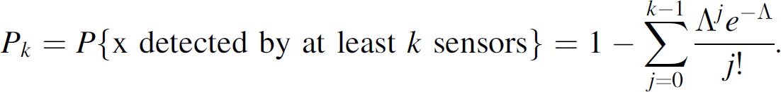
If an arbitrary point in the region is to be detected by at least k sensors, then the result shows the intensity level (i.e., Λ) that is required to achieve this performance, on average, for a given P_k. Since the mean number of sensors that detect an arbitrary point in Ω is $\mathrm{\Lambda }{\bar{A}}_S=\lambda \pi {\int }_0^{\mathrm{\infty }}{r}^{2}f(r)dr=\mathrm{\Lambda }$ , one can adjust λ (by increasing the number of sensors per unit area scattered throughout Ω) to achieve the desired coverage. The only thing that is required is some estimate of f(r), the density function describing how the detection range varies from sensor to sensor. We note that this simple adjustment is possible due to the one-to-one nature of the expression in Eq. (5). In particular,

$$\frac{d{P}_k}{d\mathrm{\Lambda }}=\frac{{\mathrm{\Lambda }}^{k-1}}{(k-1)!}\exp (-\mathrm{\Lambda })>0$$

(6)

which, along with $\mathrm{\Lambda }=\lambda {\bar{A}}_S$ , proves the one-to-one correspondence between λ and P_k for fixed average sensor coverage ${\bar{A}}_S$ .

2.3. Resulting Network Performance

Within the sensor network performance model, we recall the fact that the sensors are not necessarily perfect, they are not even necessarily identical in performance quality. In particular, f(r) (the distribution density function for the detection range over all sensors) provides a mechanism for capturing this variability. In practice, the variability may be due to manufacturing considerations and/or lack of calibration that allows the per-sensor cost to be kept down. Thus, instead of a few very expensive sensors with known fixed detection range r₀, the network may contain many less expensive sensors having uncertain detection ranges. We expect our model to illustrate this distinction and provide the appropriate conditions under which the network of inexpensive sensors performs as well as the network of fewer expensive sensors.

Through sampling, one can get an estimate of the distribution for sensor detection range. In the idealized case, in which all sensors have identical (fixed) detection range r₀, the sensor range density is given by the dirac delta function $f(r)=\delta (r-r_0)$ , such that the expected range is given by $E\{r\}=\int rf(r)dr=r_0$ . Henceforth, we refer to such idealized systems (with all sensors having identical detection range sensitivity) as homogeneous. For example, consider a homogeneous system with all sensors having identical range sensitivity r₀ = 3 units. All sensors in this network detect everything within 3 units of their location; whatever is outside of there 3 units of a sensor location is undetected by that sensor. An alternative heterogeneous system under consideration is one where the range to detection (over all sensors) follows a beta-type density:

$$f(r)=\frac{\mathrm{\Gamma }(\alpha +\beta )}{\mathrm{\Gamma }(\alpha )\mathrm{\Gamma }(\beta )}\frac{1}{c}(r/c{)}^{\alpha -1}(1-r/c{)}^{\beta -1},r\in [0,c],\alpha ,\beta >0.$$

(7)

The beta-type density model is used to convey the idea that some sensors will perform better than others. Figure 1 shows three examples of beta-type densities with realizations over the interval 0 ≤ r ≤ c where c = 5. The leftmost density in Fig. 1 (for α = 2.0 and β = 7.0) depicts the case where almost all sensors have weak detection performance. The center density in Fig. 1 depicts the opposite: for fixed β, as α increases, the density approaches the dirac delta density δ(r −5) corresponding to the homogeneous field. The rightmost density in Fig. 1 (α = 1.0 and β = 0.67) is used for the heterogeneous field in Fig. 2. This density slowly increases over most of the interval. Hence its samples are somewhat uniform over the interval with preference to samples from the upper end of the interval. It conveys the idea that, upon deployment, some sensors will be defective or give very poor performance, whereas others will perform very well. And, of course, several will provide just average performance.

Figure 1.

Sample β-type density functions.

Figure 2.

Sample homogeneous and heterogeneous sensor fields with same mean sensor detection range. The homogeneous field has r₀ = 3 and the heterogeneous has f(r) given by a beta distribution with α = 1.0, β = 0.67, c = 5.0.

The mean range to detection for this heterogeneous system is given by

$$E\{r\}={\int }_0^{c}rf(r)dr=\frac{\alpha c}{\alpha +\beta }$$

(8)

which is identical to that of the homogeneous system (where E{r} = r₀) when β = α(c −r₀)/r₀. For a maximum detection range of c = 5 units, we have an identical mean range performance of E{r} = 3 for the case of (α, β, c) = (1,0.67,5). Figure 2 shows a sample field for both the homogeneous and heterogeneous fields with approximately ² 100 sensors randomly distributed over a 100 by 100 square unit area. In this figure, both fields have the same sensor positions; however, the sensor detection ranges (represented by disk radii) are sampled from the corresponding sensor detection range distributions f(r), i.e., the dirac delta function for the homogeneous field and formula (7) for the heterogeneous field. Using the predicted coverage of Eq. (3), we compute the predicted coverage for each of these fields to be ρ _hom = 0.246 for the homogeneous field and ρ _het = 0.297 for the heterogeneous field. From the geometry of the specific fields in Fig. 2, we also compute the actual coverages (taken as the fraction of the region Ω that is covered by at least one disk) to be ${\hat{\rho }}_{hom}=0.246$ and ${\hat{\rho }}_{het}=0.295$ . We remind the reader that the sensor fields realized in Fig. 2 constitute just one possible realization of the homogeneous and heterogeneous networks under the respective detection range densities. Figure 3 displays the coverage provided by 250 randomly generated systems of each type.

Figure 3.

Two hundred and fifty simulations of the coverage for homogeneous and heterogeneous sensor fields over a 100 by 100 square unit area. The homogeneous field has detection range r₀ = 3 linear units for all sensors and the heterogeneous has detection range density f(r) given by a beta-type distribution with α = 1.0, β = 0.67, c = 5.0.

The performance of the field coverage, as given by equation (3), depends on the sensor detection range distribution density f(r) only through the expected sensor coverage area ${\bar{A}}_s$ . For the homogeneous field with $f(r)=\delta (r-r_0)$ we have

$$\begin{array}{rl}{\bar{A}}_S& =\pi {\int }_0^{\mathrm{\infty }}{r}^2\delta (r-r_0)dr\\ \hspace{0.5em}& =\pi r_0^2,\end{array}$$

(9)

which is to be expected since, for the homogeneous case, all sensors have identical detection range r₀.

For the heterogeneous field with f(r)given by a beta-type distribution as in formula (7), we have

$$\begin{array}{rl}{\bar{A}}_S& =\frac{\pi \mathrm{\Gamma }(\alpha +\beta )}{\mathrm{\Gamma }(\alpha )\mathrm{\Gamma }(\beta )}\frac{1}{c}{\int }_0^c(r/c{)}^{\alpha -1}(1-r/c{)}^{\beta -1}{r}^{2}dr\\ \hspace{0.5em}& =\frac{\pi \alpha (\alpha +1)c^2}{(\alpha +\beta )(\alpha +beta+1)},\end{array}$$

(10)

for the mean sensing area. This expression illustrates some important characteristics of heterogeneous fields. In particular, in the case of sensors with f(r) following a beta-type distribution but having the same mean detection range as the “perfect” sensors (i.e., ac/(α + β) = r₀), the mean sensing area ${\bar{A}}_S$ becomes

$${\bar{A}}_S=\pi r_0^2\left(\frac{\alpha +1}{\alpha +r_0/c}\right),$$

(11)

after substitution of β = α(c − r₀)/r₀, as shown above. Since c > r₀ (required to enforce β > 0), we see that the resulting mean sensing area ${\bar{A}}_S$ is always larger than that of the corresponding homogeneous system of same mean sensor detection range, regardless of the specific selection of α and β. Thus, the additional performance of the high-performing (range greater than r₀) sensors more than compensates for the loss in performance due to the low-performing (range less than r₀) sensors, even though the mean range is the same for both systems. Figure 4 illustrates this performance improvement in sensor field coverage for a heterogeneous field with (α, β, c) = (1.0,0.67,5.0) (yielding a mean range of 3.0) compared to a homogeneous field of sensors with r₀ = 3.0.

Figure 4.

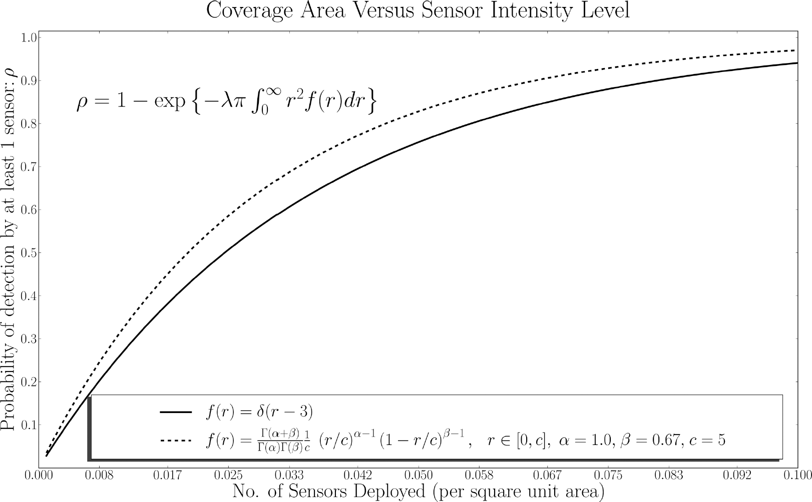
Comparison of expected coverage for homogeneous and heterogeneous sensor fields. The homogeneous field has r₀ = 3 and the heterogeneous has f(r) given by a beta distribution with α = 1.0, β = 0.67, c = 5.0.

One of the primary motivations for the employment of a heterogeneous set of sensors is the potential cost savings from using non-ideal sensors. To examine this benefit, consider a set of sensors designed with an ideal sensing range r₀. Due to manufacturing uncertainties and component irregularities, the resulting sensors do not achieve the ideal performance, but rather, may have a performance driven by a beta-type distribution with maximal range c = r₀. From (10) we see that the mean sensing area for this type of heterogeneous system is given by

$${\bar{A}}_S=\pi r_0^2\left[\frac{\alpha (\alpha +1)}{(\alpha +\beta )(\alpha +\beta +1)}\right]<\pi r_0^2.$$

(12)

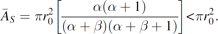
The inequality results from applying the constraints from (7) that α > 0 and β > 0. Thus, for any selection of distribution parameters, the mean sensing area performance cannot match that of the perfect sensors. However, recall from Eqs. (2), (4), and (5) that the sensor field performance is monotonically related to Λ, which is a simple product of the mean sensor coverage area ${\bar{A}}_S$ , the number of sensors N, and some constants. Thus, if a system requires N = N₀ perfect sensors with r = r₀ to achieve some needed performance, then the same average performance can be achieved with N = N_∗ imperfect sensors, where N_∗ is given by

$$N_{\ast }=N_0\left[\frac{(\alpha +\beta )(\alpha +\beta +1)}{\alpha (\alpha +1)}\right]$$

(13)

and the heterogeneous sensors have range that follows a beta distribution with maximum c = r₀ and parameters (α, β). If the per-sensor cost savings are enough that this increased number of heterogeneous sensors are cheaper than the similar field of perfect sensors, then the heterogeneous alternative becomes a cost-effective employment strategy.

We close this section by pointing out that these methods may be generalized to compare the performance of any two sensor fields. For example, suppose S₁ is a sensor field with intensity parameter λ₁ and detection range density function f₁. If S₂ is another sensor field with detection range density f₂, then the field intensity required in order to achieve, on average, the same coverage as S₁ is

$${\lambda }_2={\lambda }_1\left[\frac{{\int }_0^{\mathrm{\infty }}{r}^2{f}_1(r)dr}{{\int }_0^{\mathrm{\infty }}{r}^2{f}_2(r)dr}\right].$$

(14)

Stated differently, if system S₁ has N₁ sensors, then the number of system S₂ sensors required to achieve the same coverage, on average, is

$$N_2=N_1\left[\frac{{\int }_0^{\mathrm{\infty }}{r}^2{f}_1(r)dr}{{\int }_0^{\mathrm{\infty }}{r}^2{f}_2(r)dr}\right].$$

3. System Reliability

In this section, the reliability of the sensor network system over time is examined. Two scenarios are considered. In the first case, we analyze the change in k-coverage (k or more sensors detect an arbitrary point) of the network as sensors randomly fail. In the second scenario, we consider the system coverage as the detection capability for each sensor decays with time. This situation can occur, for example, as a result of battery depletion. Both scenarios result in reduced coverage; however, the techniques of the latter section allow for the possibility that the depleted sensors are recharged, or that the network is seeded with new sensors. While methods such as those in [19] look at extending sensor network reliability via scheduling, our focus is on surveillance in adversarial regions. In these regions, it is difficult to regularly communicate with and/or re-populate the sensors within the field. Thus, we only consider the situation in which all sensors within the field are expected to be available for sensing at all times after deployment.

3.1. Sensor Failure

We assume that the sensor lifetimes T_i are independent and identically distributed. Special attention is given to the case where the sensor lifetimes follow a Weibull distribution with scale and shape parameters μ and ν, respectively. Thus $T=T_i\sim W(\mu ,\nu )$ with failure time density

$$f_T(t)=\{\begin{array}{ll}\frac{\nu }{\mu }{\left(\frac{t}{\mu }\right)}^{\nu -1}\exp \{-(t/\mu {)}^{\nu }\},& t\ge 0\\ 0,& otherwise.\end{array}$$

(15)

The Weibull and, other gamma-type distributions, are often used in reliability theory to model the time to failure or life expectancy of electronic systems. They are particularly suited to cases where the failure mechanisms correspond to events that occur with observable (or predictable) rates. Such failure modes have been noted in sensor networks for military surveillance applications, as noted in [20].

Under the Weibull failure model, the probability that a particular sensor survives beyond time τ is

$$\begin{array}{rl}P\{T>\tau \}& ={\int }_{\tau }^{\mathrm{\infty }}{f}_T(t)dt\\ \hspace{0.5em}& =\exp \{-(\tau /\mu {)}^{\nu }\}.\end{array}$$

(16)

Thus, under the independence assumption, if N sensors are initially distributed, then the number to survive beyond time τ is a Binomial random variable with parameters N and P{T > τ}. Moreover, NP{T > τ} is the expected number of sensors to survive beyond time τ. Therefore the updated estimate for the sensor field intensity parameters (λ and Λ) are

$$\lambda (\tau )=\frac{NP\{T>\tau \}}{\parallel \mathrm{\Omega }\parallel }$$

(17)

$$\mathrm{\Lambda }(\tau )=\lambda (\tau ){\bar{A}}_S,$$

(18)

where $\parallel \mathrm{\Omega }\parallel$ is the size of the surveillance region. Due to sensor failure, the coverage statistic ρ (the probability of at least one detection) will also change over time. This section examines this change with particular attention given to the time taken for ρ(t) to decay to $100\eta \mathrm{\%}(0<\eta <1)$ of its initial value.

Let C(τ) be the number of sensors that cover an arbitrary point in Ω at time τ. The k-coverage system statistic at time τ is defined as the probability that k or more sensors detect an arbitrary point in Ω at time τ:

$${\rho }_k(\tau )\doteq P\{C(\tau )\ge k\}.$$

(19)

Similarly, we define the k-coverage system η-life, τ _k , η, as the time taken for the network k-coverage to degenerate to the fraction η of its original coverage level. That is,

$${\tau }_{k,\eta }\doteq inf\{t:{\rho }_k(t)=\eta {\rho }_k(0)\}.$$

(20)

The k-coverage system half-life is denoted by τ _{k 1/2}.

As an example of the k-coverage system η-life, we consider the 1-coverage system half-life associated with a Weibull failure model. First note that if the sensor failure rate is T ∼ W(μ, ν), then P{T > τ} is given as in Eq. (16). Now the 1-coverage system half-life occurs at τ_1,1/2 satisfying ρ₁(τ_1,1/2) = ρ₁(0)/2, i.e., from Eq. (3),

$$1-\exp \{-\mathrm{\Lambda }({\tau }_{1,1/2})\}=\frac{1}{2}(1-\exp \{-\mathrm{\Lambda }(0)\}).$$

(21)

Solving this equality for $\mathrm{\Lambda }({\tau }_{1,1/2})$ and using Eqs. (17) and (18), we obtain

$$P\{T>{\tau }_{1,1/2}\}=\frac{\parallel \mathrm{\Omega }\parallel \log [\frac{1}{2}+\frac{1}{2}\exp \{-\mathrm{\Lambda }(0)\}]}{N{\bar{A}}_S}.$$

(22)

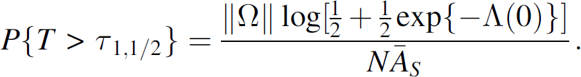
Finally, using (16), we solve explicitly for ${\tau }_{1,1/2}$ _1,1/2 as

$${\tau }_{1,1/2}=\mu {[-\log [-\frac{\log (\frac{1}{2}+\frac{1}{2}\exp (-\lambda (0){\bar{A}}_S))}{\lambda (0){\bar{A}}_S}]]}^{1/\nu }.$$

(23)

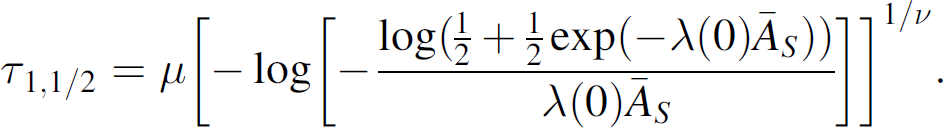
Fig. 5 shows the theoretical (solid black curve) and five simulations of the 1-coverage degradation over time of a network consisting of 250 sensors (distributed over a 100 by 100 square unit area). All sensors have a detection range of r₀ = 3 units and a failure rate modeled by a Weibull distribution with (μ, ν) = (12.5,2.25).

Figure 5.

1-Coverage degradation for a network of 250 sensors distributed over 100 by 100 square unit area. Sensor failures occur randomly, following a Weibull distribution with parameters μ = 12.5, ν = 2.25.

In general, the η-life k-coverage for the system lifetime must be solved numerically. For example, consider τ _k,η , the time taken for the system k-coverage to decay to 100η % (0 < η < 1) of its original coverage level. From formula (5), it follows that

$${\rho }_k(\tau )=1-(1+\mathrm{\Lambda }(\tau )+\dots +\frac{{\mathrm{\Lambda }}^{k-1}(\tau )}{(k-1)!})\exp \{-\mathrm{\Lambda }(\tau )\}.$$

(24)

We are interested in τ _k,η satisfying ρk(τ _k,η ) = ηρ _k (0). That is,

$$\begin{array}{rl}\hspace{0.5em}& 1-(1+\mathrm{\Lambda }({\tau }_{k,\eta })+\dots +\frac{{\mathrm{\Lambda }}^{k-1}({\tau }_{k,\eta })}{(k-1)!})\exp \{-\mathrm{\Lambda }({\tau }_{k,\eta })\}\\ \hspace{0.5em}& =\eta [1-(1+\mathrm{\Lambda }(0)+\dots +\frac{{\mathrm{\Lambda }}^{k-1}(0)}{(k-1)!})\exp \{-\mathrm{\Lambda }(0)\}].\end{array}$$

(25)

Or equivalently, after collecting terms,

$$\begin{array}{rl}-\mathrm{\Lambda }({\tau }_{k,\eta })& +\log (1-\mathrm{\Lambda }(r_{k,\eta })\dots +\frac{{\mathrm{\Lambda }}^{k-1}({\tau }_{k,\eta })}{(k-1)!})\\ \hspace{0.5em}& =\log [(1-\eta )+\eta (1+\mathrm{\Lambda }(0)+\dots +\frac{{\mathrm{\Lambda }}^{k-1}(0)}{(k-1)!})\exp \{-\mathrm{\Lambda }(0)\}].\end{array}$$

(26)

Now, for given η, the right hand side of (26) is constant. Therefore, we can set

$$y_{\eta }=\log [(1-\eta )+\eta (1+\mathrm{\Lambda }(0)+\dots +\frac{{\mathrm{\Lambda }}^{k-1}(0)}{(k-1)!})\exp \{-\mathrm{\Lambda }(0)\}],$$

(27)

and solve (numerically)

$${\hat{\mathrm{\Lambda }}}_{k,\eta }-\log (1+{\hat{\mathrm{\Lambda }}}_{k,\eta }\dots +\frac{{\hat{\mathrm{\Lambda }}}_{k,\eta }^{k-1}}{(k-1)!})+y_{\eta }=0$$

(28)

for ${\hat{\mathrm{\Lambda }}}_{k,\eta }$ . Note that any solution to (28) also solves (26) with $\mathrm{\Lambda }({\tau }_{k,\eta })$ equal to ${\hat{\mathrm{\Lambda }}}_{k,\eta }$ . Thus, we set $\mathrm{\Lambda }({\tau }_{k,\eta })={\hat{\mathrm{\Lambda }}}_{k,\eta }$ and use (17)–(18) to solve for τ_k,η:

$$\begin{array}{rl}{\hat{\mathrm{\Lambda }}}_{k,\eta }& =\mathrm{\Lambda }({\tau }_{k,\eta })\\ \hspace{0.5em}& =\frac{NP\{T\ge {\tau }_{k,\eta }\}}{\parallel \mathrm{\Omega }\parallel }{\bar{A}}_S.\end{array}$$

(29)

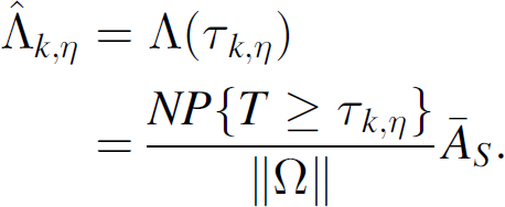
Hence the k-coverage η-lifetime, ${\tau }_{k,\eta }$ , satisfies

$$P\{T\ge {\tau }_{k,\eta }\}=\frac{{\hat{\mathrm{\Lambda }}}_{k,\eta }\parallel \mathrm{\Omega }\parallel }{N{\bar{A}}_S}.$$

(30)

In the particular case where the sensor failure rate follows a known distribution, we can solve (30) explicitly for τ_k,η. For example, recall (see Eq. (16)) that for the Weibull sensor failure rate $P\{T\ge {\tau }_{k,\eta }\}=\exp \{-({\tau }_{k,\eta }/\mu {)}^{\nu }\}$ . Therefore,

$${\tau }_{k,\eta }=\mu {\left[\log \left[\frac{N{\bar{A}}_S}{{\hat{\mathrm{\Lambda }}}_{k,\eta }\parallel \mathrm{\Omega }\parallel }\right]\right]}^{1/\nu }$$

(31)

$$=\mu {\left[\log \left(\frac{\lambda \pi {\int }_0^{\mathrm{\infty }}{r}^{2}f(r)dr}{{\hat{\mathrm{\Lambda }}}_{k,\eta }}\right)\right]}^{1/\nu }.$$

(32)

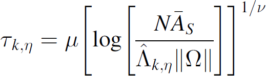
Fig. 6 compares the degradation for the 1, 2, and 3-coverage for a network of 500 homogeneous sensors. In all of the examples in Fig. 6, the degradation follows a Weibull distribution with parameters (μ, ν) = (12.5, 2.25). Note that the graphs start out essentially flat, due to few sensor failures at the time of deployment. Note also that the k-coverage half-life decreases with increasing k. This is to be expected since coverage overlap decreases as the sensors randomly die off.

Figure 6.

k-coverage degradation for a network of 500 homogeneous sensors distributed over 100 by 100 square unit area. Sensor failures occur according to a Weibull distribution with parameters (μ, ν) = (12.5, 2.25).

Equation (30) describes the relationship between N, the number of sensors initially distributed, and τ_k,η, the time taken for the system k-coverage to degrade to a fraction η of the initial coverage. It is desirable to know the number of sensors to deploy in order to guarantee a certain level of performance at some future time. This can be found by solving Eq. (30) for N. Recall, however, from (17)–(18) that ${\hat{\mathrm{\Lambda }}}_{k,\eta }$ depends on N; hence it is not simple to solve (30) for N. However, Eq. (30) can be used to determine the number of initial sensors N required in order to have the k-coverage degrade, on average, to 100η% of its initial value after τ∗ time units. That is, Eq. (30) can be used to determine τ_k,η(N)for increasing levels of N until a value N_τ∗ satisfying τ_k,η(N_τ∗) > τ∗ is reached.

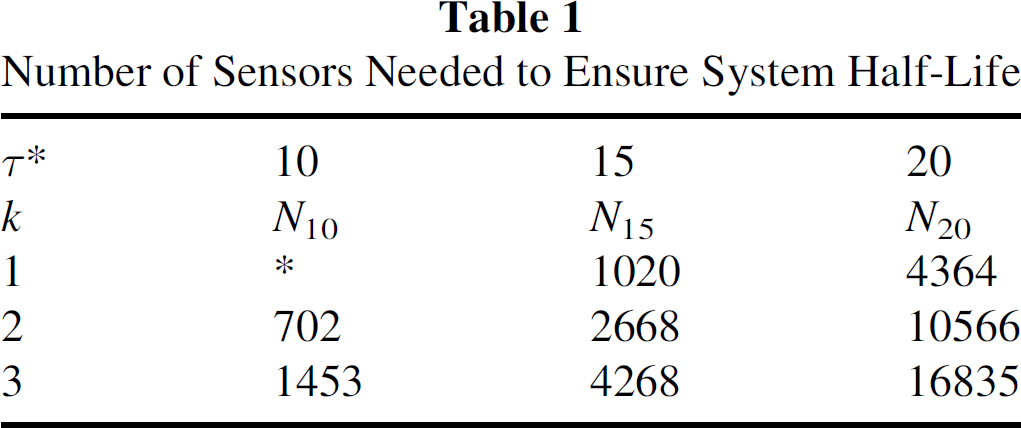
Table 1 shows the required values of N_τ∗ for k = 1,2, and 3 to achieve various levels of τ∗. For this example, all sensors have a detection range of 3 units, and the life expectancy of the sensors is assumed to follow a Weibull distribution with parameters μ = 12.5 and ν = 2.25. The surveillance region is a 100 by 100 square unit area. The asterisk in row one signifies that, under the given parameters for the sensor life expectancy, the expected 1-coverage for any number of distributed sensors is greater than ten time units. The mean value of a Weibull random variable with parameters (μ, ν) = (12.5, 2.25) is μ(1 + 1/ν) = 11.07. Therefore, on average, a network consisting of just one sensor will maintain coverage up to 10 time units after deployment. Moreover, the expected system k-coverage (for any k) increases with increasing N. This occurs due to the following: For any number of sensors initially deployed, points in the space are covered by either fewer than k sensors, or are covered by at least k sensors. If additional sensors are immediately (i.e., no time passes between the initial and secondary deployment) added to the field, then some points previously not covered by k sensors will attain m-coverage, m ≥ k. Over time, these points will lose their k-coverage at a rate no greater than points previously covered by exactly k sensors. Some points already covered by at least k sensors (i.e., before the additional sensors were deployed) will acquire additional coverage; these points will lose their k-coverage at a slower rate than they would without the additional sensors.

TABLE 1

Number of Sensors Needed to Ensure System Half-Life

τ∗	10	15	20
k	N 10	N 15	N 20
1	∗	1020	4364
2	702	2668	10566
3	1453	4268	16835

3.2. Degrading Range Sensitivity and Field Reseeding

Due to limited battery supply and the autonomous nature of the distributed sensors, it is expected that degrading range sensitivity is a more prevalent reliability issue (especially over extended periods of operation) than simple failure. In this section we consider the field performance for the situation where sensor effectiveness degrades with time.

Although the field intensity parameter λ is constant, the detection range density across all sensors and the mean sensor detection parameter are functions of time, denoted F(r; τ) and 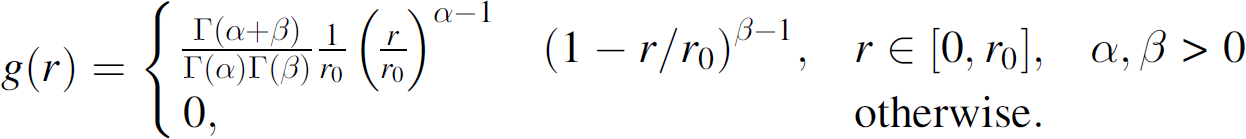$\mathrm{\Lambda }(\tau )$ , respectively. Suppose, for example, that the homogeneous sensors all start out with an ideal sensor detection range of r₀ units. Suppose also that, over time, the sensor effectiveness across the entire field decays in a manner such that the terminal detection range for each sensor follows a beta-type distribution:

$$g(r)=\{\begin{array}{ll}\frac{\mathrm{\Gamma }(\alpha +\beta )}{\mathrm{\Gamma }(\alpha )\mathrm{\Gamma }(\beta )}\frac{1}{r_0}{\left(\frac{r}{r_0}\right)}^{\alpha -1}(1-r/r_0{)}^{\beta -1},& r\in [0,r_0],\alpha ,\beta >0\\ 0& \text{otherwise}.\end{array}$$

(33)

An initial-terminal range analysis can be used to determine a lower bound on the network performance over time.

As time progresses, the network evolves into a mixture of the initial and terminal sensor systems with density

$$\mathcal{F}(r;\tau )=\mathrm{\Phi }(\tau )\delta (r-r_0)+(1-\mathrm{\Phi }(\tau ))g(r),$$

(34)

where $\mathrm{\Phi }(\tau )=P\{T>\tau \}$ . That is, the evolving detection range density is a mixture of ranges for those sensors which have already degraded and those which have yet to undergo diminished performance. The evolving coverage statistic ρ(τ) and mean sensor area coverage ${\bar{A}}_S(\tau )$ are now temporally varying according to

$$\rho (\tau )=1-\exp \{-\mathrm{\Lambda }(\tau )\}$$

(35)

$${\bar{A}}_S(\tau )=\pi {\int }_0^{\mathrm{\infty }}{r}^2\mathcal{F}(r,\tau )dr$$

(36)

where $\mathrm{\Lambda }(\tau )=\lambda {\bar{A}}_S(\tau )$ . Formula (35) provides an estimate of the coverage statistic ρ(τ) over time.

With little effort, F (r;τ) can also be adjusted to account for additional sensors randomly distributed over the field. For example, suppose M additional sensors are added to the field at time τ∗. Then the proportion of all sensors to have undergone change at time τ > τ_∗ is

$$\mathrm{\Phi }(\tau )=\frac{N}{N+M}P\{T>\tau \}+\frac{M}{N+M}P\{T>(\tau -{\tau }_{\ast })\},$$

(37)

where, as before, N is the number of sensors originally distributed over the surveillance field. Recall that Φ(τ), as used in (34), is interpreted as the proportion of items that have yet to experience diminished effectiveness. With the added sensors, the total number in the field includes those from the original N as well as from the new set which have yet to change. At time τ ≥τ_∗, the proportion from the original set that have yet to experience reduced effectiveness is P{T > τ}. The new sensors did not exist before time τ_∗, therefore the proportion for these sensors is P{T > (τ – τ_∗)}. Thus, for all N + M sensors, the proportion from the entire set that have yet to experience reduced effectiveness is given by formula (37).

Using the decay mixture described by equation (34) with the corresponding end state of Eq. (33), the mean sensor area coverage reduces to

$${\bar{A}}_S(\tau )=\pi r_0^2+\pi r_0^2[\frac{\alpha (\alpha +1)}{(\alpha +\beta )(\alpha +\beta +1)}-1](1-\mathrm{\Phi }(\tau )).$$

(38)

Figure 7 shows the coverage degradation over time of the predicted result (dark line) and five simulations of a sensor network in which range sensitivity degrade from a homogeneous network (all sensors have detection range of 3 units) to a heterogeneous network (detection over all sensors decay to samples from a beta-type distribution of the form of equation (7) with (α, β) = (2,2)). The time to decayed performance for each sensor follows a Weibull distribution with parameters (μ, ν) = (12.5, 2.25). After 15 time units the field is recharged with the addition of another 125 homogeneous sensors. From Fig. 7, it is clear that the re-seeded field does not behave identically to the initial field, although it does reach the same peak level. In particular, note that the slope of the decay in performance after reseeding is greater than that initially. This is an important feature of maintaining many aged sensors in the field, and is a critical component of the model for sensor deployment planning purposes.

Figure 7.

System Degradation with Reseeding.

4. Conclusion

A mathematical model has been presented to examine the coverage and reliability of distributed sensor networks that are designed for surveillance applications. The model uses established methods of sensor network coverage analysis that are based on Poisson processes, and extends them with known reliability models to provide estimates of field degradation over time. Examples were presented that show the required numbers of initially deployed sensors to maintain coverage over extended periods of operation, as well as how to choose appropriate re-seeding of a field that has degraded. When used in conjunction with appropriate cost models, the methods of this paper can be utilized to derive optimal deployment strategies for surveillance application of distributed sensor networks.