Sage Journals: Discover world-class research

Abstract

Distributed sensor fields have recently gained popularity as a means for detecting intruders moving through a protected area of the ocean. We characterize the detection capabilities of a network of randomly-deployed sensors with varying sensing capabilities. We develop a framework for analytically approximating the probability that such a sensor field detects a constant course target moving through the region as a function of the number of sensors deployed and the statistical properties that govern the sensing range. Analytical and empirical results indicate that, when the total sensing area is fixed, a set of smaller distributed sensors can achieve significantly improved detection performance relative to a single large sensor. We also study the relationship between coverage of a region of interest and likelihood of detecting a constant course intruder moving through that region. We derive expressions for the average number of sensors required to achieve a prescribed likelihood of detection and level of coverage and conclude that detection and coverage are fundamentally different characterizations of the capabilities of a sensor field. In fact, the number of sensors required to achieve a particular detection level may be several orders of magnitude smaller than that required to achieve the same level of coverage.

Keywords

Distributed Sensor Networks Heterogeneous Sensor Field Spatial Poisson Process Detection Versus Coverage

1. Introduction

The first line of defense for protecting a defined region of the ocean, often called a sea base, is a system consisting of sensors and the associated signal processing that perform detection, classification, localization, and tracking (DCLT). We are engaged in the basic research needed to inform the development of SONAR system technology that can be used to determine if underwater objects (fish, mines, submarines, or underwater vehicles) are present in the volume of water constrained within, for example, a square area of the ocean. Traditionally, DCLT tasks have been performed by large, expensive sensor platforms with sophisticated signal processing capabilities that result in long detection ranges. Recent advances in the detection capabilities of commercial networks composed of small, low-cost wireless sensors [1, 2] have raised the possibility of similar approaches in an underwater environment. These approaches, called undersea distributed networked systems (UDNS), are becoming a research topic of significant interest in the underwater community [3].

A chief goal of our work is to characterize the performance of randomly-distributed sensor fields for detection of an intruder moving through the region of interest. Much of the existing research on the capabilities of such sensor fields has focused on coverage, or equivalently, the probability that a particular point in the region is within the sensing region of at least 1 (or perhaps at least k) sensors. Onur et al. [4] present an analytical expression for the probability that a random point in a rectangular region is detected by at least one of N identical randomly-deployed sensors. Additional coverage measures such as breach and support are defined in [5], and algorithms for identifying paths that achieve maximum breach and minimum support under known sensor placement are developed in [5] and [6]. In [7], the concept of coverage is extended to consider moving targets by quantifying the coverage along an arbitrary path through the region of interest. Liu et al. [8] compute the probability that an object moving between two points in a region can be detected by a homogeneous network of randomly-deployed sensors as a function of the length of the path traveled. In both [7] and [8], an infinite region of interest is assumed in generating analytical results, and hence edge effects are not incorporated. Clouqueur et al. [9] also consider detection capabilities for moving targets but with a focus on algorithmic strategies for deploying sensors in the region of interest.

Our work differs from that described above in that it focuses purely on quantifying the probability of detecting a moving target (rather than on coverage statistics for the region or for a target path) within a bounded region of interest using a field of randomly-deployed sensors, directly addressing the effects of boundary conditions on detection capabilities. In work that has studied detection directly, analysis has focused on the detection capabilities of sparsely distributed sensors whose sensing regions are assumed not to overlap [10]. In [11], for example, Traweek and Wettergren characterize the sensing range that optimizes the detection vs. cost trade-off in a sparse sensor field. In contrast to previous work, we consider how to choose the number and sophistication of sensors to maximize detection performance when sensor placement is random. Such a model is particularly relevant when small, low-cost sensors are used, since deployment may be as simple as dropping sensors from a moving platform, such as a plane or surface ship. Once deployed in the ocean environment, floating sensors will be relocated by waves, tides, and other ocean forces. An additional complexity occurs when individual sensors within the network vary with respect to detection capabilities, specifically the sensing range. Such variability may be introduced intentionally when sensors of differing sophistication are incorporated in a heterogeneous network. Consider, for example, a network composed of submarines, unmanned vehicles, sonobuoys, and low-cost floating (un-tethered) sensors. Each type of sensor is expected to provide different detection capabilities, in correlation with their respective costs of production and operation. Alternatively, variability may be introduced through manufacturing uncertainties, e.g., variations in the performance of a batch of sensors designed to meet certain specifications. In many scenarios, especially when a large number of sensors are deployed, it is impractical to test each sensor prior to deployment, and hence sensors with varying capabilities will be used. Even if testing of all sensors is possible, removing sensors that fail to meet design specifications is an inefficient approach, since even lower-performing sensors (whose cost of production has already been paid) can contribute to the overall detection capabilities of the network. In our work, we explore detection performance as a function of both the number of sensors deployed and their individual detection radii. We are interested in exploring the performance of such systems in the limit as the number of sensors grows and their respective sophistication/cost decreases. A related engineering and production challenge, of course, is to deliver small, reliable sensors at low cost, an important topic beyond the scope of this article.

The remainder of the article is organized as follows. A model for the system under consideration is presented in Section 2. The likelihood of detection using a single sensor placed at the center of a square sea base is derived in Section 3. The likelihood of detection for randomly-distributed heterogeneous sensors is derived in Section 4, and the generalization beyond a square sea base to arbitrary convex regions is discussed. The relationship between coverage and detection for randomly placed sensors is discussed in Section 5, and conclusions are drawn in Section 6.

2. System Model

We consider sensors that have a disc-shaped detection region, e.g., omnidirectional sensing. The range of a sensor's detection region is given by its sensing radius r₀, which we assume is a random variable drawn from some known probability density function f(r). Thus the detection range, and hence the detection region, varies from sensor to sensor. A sensor network field of this type, with heterogeneous sensing radii, adds an additional level of complexity to the analysis: not only are the sensor locations random, but the actual coverage area of each sensor is also random. Variation in sensor range might occur, for example, as sensor performance degrades over shelf life or as new models are introduced with improved performance [12]. When all sensors are assumed to have the same known sensing radius r₀, the probability density function simply reduces to f(r) = δ(r − r₀), where δ denotes the Dirac delta function. In all cases, a Boolean sensing model is assumed [13]: a sensor detects a moving target with probability one if the intruder's path intersects the sensing region of that sensor. Expanding the sensor operating model to characterize the effect of detection as a function of time spent in the sensing region and false alarm rates is an important topic but lies outside the scope of this paper.

Randomly scattered sensors are assumed to be spatially distributed according to a Poisson point process [14] with parameter λ. A spatial Poisson process provides a model for the number of points associated with a particular event over a region of space. For example, suppose Ω denotes an n-dimensional set, and let A ⊂ Ω. Consider points scattered randomly throughout Ω, and let $N (A)$ denote the number of points that are contained in A. Then the random process $N = {N (A), A \subset Ω}$ is called a point process in Ω. Let ‖A‖ denote the volume of A. The stochastic process $N = {N (A), A \subset Ω}$ is an n-dimensional Poisson counting process with parameter λ > 0 if

N(A) follows a Poisson distribution with mean λ ‖A‖, and

The number of points occurring in disjoint subsets of Ω are mutually independent.

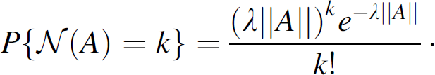
Thus, if $N = {N (A), A \subset Ω}$ is an n-dimensional Poisson counting process with parameter λ > 0, then the probability of k occurrences (of points) in the subset A is given by

P {N (A) = k} = \frac{(λ | | A | |)^{k} e^{- λ | | A | |}}{k!}

It follows from (a) that the average number of points in Ω is λ‖Ω‖, where ‖Ω‖ denotes the volume of the region Ω. A more detailed description of spatial Poisson processes can be found in [14].

One of the main goals of our work is to draw a distinction between intruder detection and region coverage as metrics for quantifying the performance capabilities of randomly-distributed heterogeneous sensor fields. Hence, we introduce sensor coverage statistics based on a Poisson point process model. For a two-dimensional region (n = 2), assuming that the sensing range for all sensors are independent of location and drawn from density f(r), the number of sensors that cover an arbitrary point x ∊ Ω is a Poisson random variable with parameter (cf., [15])

Λ = λ π \int_{0}^{\infty} r^{2} f (r) d r .

Hence, the probability that k or more sensors cover the point x ∊ Ω is equal to $Λ^{k} e^{- Λ} / k!$ , and the probability that x is covered by at least one sensor is given by

\begin{aligned} ρ & = \sum_{k = 1}^{\infty} \frac{Λ^{k} e^{- Λ}}{k!} \\ = 1 - e^{- Λ .} \end{aligned}

(1)

We refer to the statistic p as the predicted coverage for the sensor network. The coverage statistic ρ can also be interpreted as the expected proportion of the space covered by at least one sensor. We should point out that for the three-dimensional problem, we have $Λ = \frac{4}{3} λ π \int_{0}^{\infty} r^{3} f (r) d r$ however, for the remainder of this paper we will consider only the two-dimensional case.

We model the region of interest (sea base) as a square with sides of length 2U, but the techniques employed and the corresponding results can be generalized to any convex region, as will be discussed further in Section 4.2. We employ a Cartesian coordinate system in which the sea base is centered at (x, y) = (0, 0). An intruder is constrained to move at a constant course (straight line) through the sea base but can enter at any arbitrary point and travel on any arbitrary course that will take it through at least some portion of the region of interest. Without loss of generality, we assume that the intruder enters the sea base through the lower edge of the square. The intruder enters at point (u, -U) and with angle θ, where u ∊ [−U, U], and θ ∊ [0, π]. An example trajectory through the sea base is shown in Fig. 1.

Figure 1.

Example target trajectory through the sea base. Intruder enters at point (u, -U) on the lower edge of the square and with angle θ relative to the horizontal.

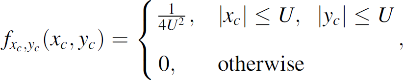
Our analysis results in an expression for probability of detection that is independent of the particular path traveled by the intruder through the sea base. To obtain this result, we model both the point u at which the intruder enters the sea base and the angle θ with which it enters as uniformly distributed random variables with probability density functions given by

f_{u} (u) = {\begin{cases} \frac{1}{2 U}, & | u | \leq U \\ 0, & otherwise . \end{cases}

and

f_{θ} (θ) = {\begin{cases} \frac{1}{π}, & 0 \leq θ \leq π \\ 0, & otherwise . \end{cases}

Figure 2 depicts four example scenarios in which heterogeneous sensors are randomly distributed over the surveillance region. While the four scenarios may appear quite different at first glance, the number of sensors and their locations are identical in each frame. What differs is the coverage, i.e., the actual sensing radius of each sensor varies from scenario to scenario. When the sensing range is a random variable, the answer to the question of whether or not an arbitrary sensor will detect a particular intruder is not binary. This can be seen in Fig. 2, as sensors at particular locations detect the intruder in some scenarios but not in others.

Figure 2.

Four examples of heterogeneous sensors randomly distributed across the surveillance region. The sensor locations are identical in each of the four frames, but each sensor's radius varies across the four scenarios.

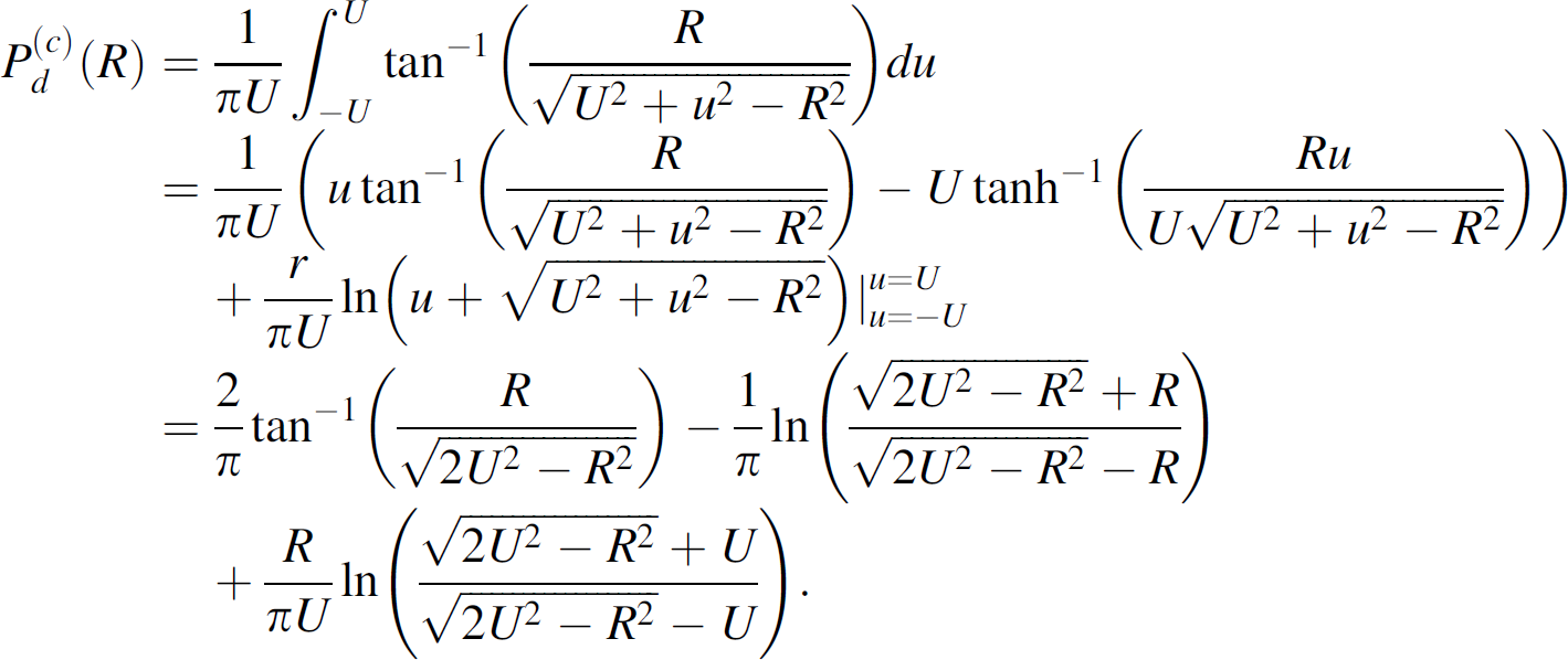
3. Likelihood of Detection Using a Single Centered Sensor

In this section, we consider the detection performance of a single sensor with sensing radius R whose center is located at the center of the sea base, e.g., (x, y) = (0, 0). Such a scenario could be used to model, for example, a submarine monitoring a particular region of the ocean. We use the single centered sensor as a baseline representation of a traditional sophisticated sensor and compare its performance to that of a randomly-deployed sensor field. Using an analytic approach, we determine the probability that the single sensor will detect an intruder moving in a straight line through the square sea base. An intruder entering the sea base at point (x, y) = (u, − U) will intersect the sensing region of the sensor if its angle of entry is within a particular range, as shown in Fig. 3. Since the distribution over the angle of entry is uniform, we need to determine (as a function of u) only the fraction of the range of entry angles from 0 to p that will result in an intersection. We denote this range of entry angles by ϕ. Creating the right triangle, we see that

\tan (ϕ / 2) = \frac{R}{\sqrt{U^{2} + u^{2} - R^{2}}}, 0 \leq R \leq U .

Figure 3.

ϕ denotes the extent of angles for which an intruder entering the sea base at point (x, y) = (u, −U) will be detected by a single sensor centered in the sea base. The two dashed lines shown create a right triangle when combined with the rightmost solid line. The length of the hypotenuse is easily computed as $\sqrt{u^{2} + U^{2}}$ , and the length of the side lying within the circle is R .

For a particular point of entry u, the probability that an intruder enters with an angle within the range ϕ for which detection occurs can then be written as

P r (θ \in ϕ | u) = \frac{2}{π} \tan^{- 1} (\frac{R}{\sqrt{U^{2} + u^{2} - R^{2}}}) .

Integrating over a uniform prior on u, we obtain the expression

\begin{aligned} P_{d}^{(c)} (R) = & \frac{1}{π U} \int_{- U}^{U} \tan^{- 1} (\frac{R}{\sqrt{U^{2} + u^{2} - R^{2}}}) d u \\ = & \frac{1}{π U} (u \tan^{- 1} (\frac{R}{\sqrt{U^{2} + u^{2} - R^{2}}}) - U \tanh^{- 1} (\frac{R u}{U \sqrt{U^{2} + u^{2} - R^{2}}})) \\ + \frac{r}{π U} \ln (u + \sqrt{U^{2} + u^{2} - R^{2}}) |_{u = - U}^{u = U} \\ = & \frac{2}{π} \tan^{- 1} (\frac{R}{\sqrt{2 U^{2} - R^{2}}}) - \frac{1}{π} \ln (\frac{\sqrt{2 U^{2} - R^{2}} + R}{\sqrt{2 U^{2} - R^{2}} - R}) \\ + \frac{R}{π U} \ln (\frac{\sqrt{2 U^{2} - R^{2}} + U}{\sqrt{2 U^{2} - R^{2} - U}}) . \end{aligned}

(2)

It is insightful to evaluate the likelihood that an intruder traveling a straight line will be detected when the sensing radius of the single sensor is equal to half the length of the square, e.g., R = U. In such a scenario, the sensing region is a circle inscribed in the square sea base, but intruders still avoid detection when traveling through a corner of the square, as shown in Fig. 4. In the limit as R approaches U from the left, we find that

\begin{aligned} P_{d}^{c} (U) = & \frac{2}{π} lim_{R \to U} [\tan^{- 1} (\frac{R}{\sqrt{2 U^{2} + R^{2}}}) - \frac{1}{π} \ln (\frac{\sqrt{2 U^{2} - R^{2}} + R}{\sqrt{2 U^{2} - R^{2}} - R}) \\ + \frac{R}{π U} \ln (\frac{\sqrt{2 U^{2} - R^{2}} + U}{\sqrt{2 U^{2} - R^{2}} - U})] \\ = & \frac{1}{2} + \frac{\ln (2)}{π} \approx .72 . \end{aligned}

Figure 4.

An intruder moving through the sea base in a straight line may avoid being detected by a sensor whose sensing radius R = U if the intruder travels through a corner of the square region.

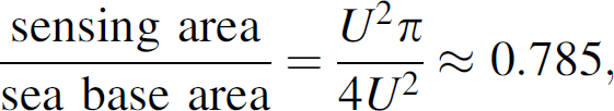
Thus, the probability that the intruder will travel through one of the corner regions and avoid detection is $1 - P_{d}^{c} (U) \approx 0.28$ . Note that this probability is independent of the size of the sea base. Note also that, because we are considering the likelihood of detecting a moving target, the probability of avoiding detection in this scenario is not equivalent to the fraction of the sea base area not covered by the sensing region of the single large sensor. In fact, the likelihood that the sensing region covers a randomly chosen point in the sea base is given by

\frac{sensing area}{sea base area} = \frac{U^{2} π}{4 U^{2}} \approx 0.785,

and hence coverage of a randomly chosen point is more likely than detection of a target following a randomly chosen straight line. We will see that this relationship is reversed (e.g., detection becomes more likely than coverage) when a network of smaller sensors is employed.

To corroborate our analytical results, the likelihood of detection for a single centered sensor has been simulated for U = 1 R between 0 and 1. For each value of R, 10⁶ independent simulations were conducted. Both the analytical and simulation results are plotted as a function of R in Fig. 5. The analytical and empirical results are nearly identical, providing two independent but consistent answers to the same question. As the sensing radius R increases beyond 1, P_d increases more slowly, reflecting the fact that much of the additional detection region falls outside the sea base.

Figure 5.

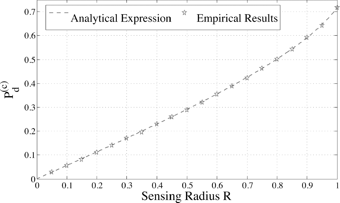
Probability that a straight-line target is detected by a single sensor with radius R centered in a square sea base with length 2U = 2. The analytical expression is plotted as a solid line; stars denote empirical results for the same parameters.

4. Likelihood of Detection using a Heterogeneous Sensor Field

4.1. Detection Probability for a Single Sensor

To derive the probability of detecting an intruder when a set of sensors with heterogeneous sensing range are randomly deployed in the sea base, we begin by deriving the probability of detection for a single randomly-placed sensor with constant sensing radius r. Let the sensor be centered at (x_c, y_c), where x_c ∊ [-U, U] and y_c ∊ [-U, U]. For an intruder entering the sea base at point (u, -U) and with angle θ, the equation of a line traveled by the target is given by

y = x \tan θ - U - u \tan θ .

The probability of detection across all sensor locations for the path defined by u and θ can be written as

P_{d | θ, u} (r) = \int_{x_{c}} \int_{y_{c}} P_{d | (x_{c}, y_{c}), 0, u} (r) f_{x_{c}, y_{c}} (x_{c}, y_{c}) d x_{c} d y_{c},

where

f_{x_{c}, y_{c}} (x_{c}, y_{c})

denotes the probability density function over the sensor location. The probability of detection for a sensor centered at (x_c, y_c) is given by

P_{d | (x_{c}, y_{c}), θ, u} (r) = {\begin{cases} 1, & d_{min} (x_{c}, y_{c}, u, θ) \leq r \\ 0, & d_{min} (x_{c}, y_{c}, u, θ) > r \end{cases},

where d_min(x_c, y_c, u, θ) denotes the minimum distance between the sensor center and the closest point on the line traveled by the target. Assuming the sensor location is uniformly distributed across the square, e.g.,

f_{x_{c}, y_{c}} (x_{c}, y_{c}) = {\begin{cases} \frac{1}{4 U^{2}}, & | x_{c} | \leq U, | y_{c} | \leq U \\ 0, & otherwise \end{cases},

we can compute P_d for a given u and θ as

P_{d | θ, u} (r) = \frac{1}{4 U^{2}} \int_{A} d x_{c} d y_{c},

(3)

where

A = {(x_{c}, y_{c}) : d_{min} \leq r, x \in [- U, U], y \in [- U, U]} .

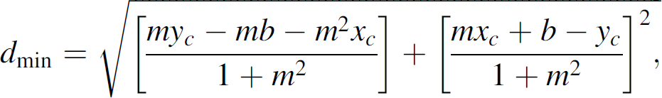
The probability that the intruder intersects the sensing region of the sensor is equal to the probability that the distance from the sensor center to the closest point on the line is less than or equal to the sensing radius of the sensor. The closest point on the target path to the sensor center is the solution to

\frac{d}{d x} (x - x_{c})^{2} + (y (x) - y_{c})^{2} = 0,

which is given by

\begin{aligned} x & = \frac{x_{c} + y_{c} \tan θ + U \tan θ + u \tan^{2} θ}{1 + \tan^{2} θ}, and \\ y & = \frac{x_{c} \tan θ + y_{c} \tan^{2} θ - U - u \tan θ}{1 + \tan^{2} θ} . \end{aligned}

The minimum distance between the sensor center and a point on the line traveled by the intruder is then computed as

d_{min} = \sqrt{[\frac{m y_{c} - m b - m^{2} x_{c}}{1 + m^{2}}] + {[\frac{m x_{c} + b - y_{c}}{1 + m^{2}}]}^{2}},

(4)

where m = tan θ and b = -U - u tan θ are the slope and y-intercept, respectively, of the target path. Rearranging (4), the region of the sea base for which

d_{min} \leq r

can be expressed in terms of x_c and y_c as

m x_{c} + b - r \sqrt{1 + m^{2}} \leq y_{c} \leq m x_{c} + b + r \sqrt{1 + m^{2}} .

Graphically, the region of interest lies between the target path shifted upward by $r \sqrt{1 + m^{2}}$ and the target path shifted downward by $r \sqrt{1 + m^{2}}$ , three examples of which are shown in Fig. 6. The perpendicular distance between the target path (center line of the shaded region) and either of the shifted paths (edge lines of the shaded region) is r. The result is intuitively pleasing, as it concludes that a sensor whose center is within distance r of the target path will detect the intruder.

Figure 6.

Possible target paths through the sea base and associated regions for which $d_{m i n} \leq r$ . The target path within the sea base is represented by the center lines. The region for which $d_{m i n} \leq r^{2}$ (darkly shaded) is between the edge lines, each of which is a shifted version of the target path. The cenarios shown are examples of case 1, 2, and 3, respectively, as defined to compute P_d(r).

The region denoted by A is simply the region that falls between the shifted paths and within the sea base, e.g., all points (x_c, y_c) within the sea base for which $d_{m i n} \leq r$ . The form of the region A depends upon which sides of the square are intersected by the ends of the shifted path segments that define the detection region; these are, in turn, determined by the point and angle at which the intruder enters the sea base, as well as by the radius, r of the sensor. Three possible scenarios are shown in Fig. 6. While it is possible to identify ranges of u and θ that uniquely define the shape of the detection region, such an approach is tedious and cumbersome. Instead, we employ an approximate approach that, as we will show, yields results that are very similar to empirical results for the range of r in which we are interested. Rather than computing the exact area of the detection region, we compute the area of the rectangle whose central axis is given by the target path within the square and whose width is given by 2r, the perpendicular distance between the edge lines of the shaded region. We denote this region by Ã. Figure 7 shows the corresponding rectangle for each of the three scenarios given in Fig. 6.

Figure 7.

Approximation to the area of the detection region defined by a rectangle whose longer central axis is defined by the length of the target path within the sea base. r is assumed to be significantly less than U.

For ease of presentation, let U = 1. To compute the length of the target path within the sea base (and hence the approximate area of the detection region), we consider three cases. For each case, the applicable ranges of u and θ, as well as the resulting area of the rectangle, are given below:

Case 1: Intruder exits right side of square.

\begin{aligned} 0 \leq θ \leq \tan^{- 1} (2 / (1 - u)) \\ ∥ {\tilde{A}}_{1} ∥ = \frac{2 r (1 - u)}{\cos θ} \end{aligned}

Case 2: Intruder exits top of square.

\begin{aligned} \tan^{- 1} (2 / (1 - u)) \leq θ \leq \tan^{- 1} (2 / (- 1 - u)) \\ ∥ {\tilde{A}}_{2} ∥ = \frac{4 r}{\sin θ} \end{aligned}

Case 3: Intruder exits left side of square.

\begin{aligned} \tan^{- 1} (2 / (- 1 - u)) \leq θ \leq π \\ ∥ {\tilde{A}}_{3} ∥ = \frac{- 2 r (u + 1)}{\cos θ} \end{aligned}

Note that Figs. 6 and 7 give examples from each of the three cases defined above.

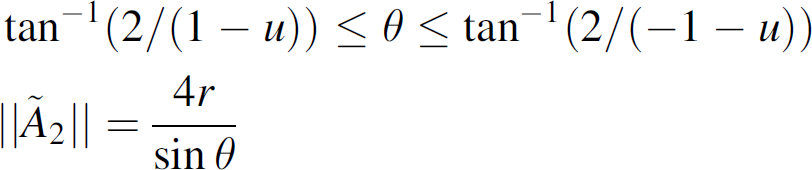
The probability of detection across all u and θ can be written as

\begin{aligned} P_{d} (r) & = \int_{u} \int_{θ} P_{d | θ, u} (r) f (θ) f (u) d θ d u \\ = \frac{1}{2 π} \int_{u = - 1}^{1} \int_{θ = 0}^{π} P_{d | θ, u} (r) d θ d u . \end{aligned}

The function to be integrated displays symmetry across $0 \leq θ \leq π / 2$ and $π / 2 \leq θ \leq π$ , and hence we can equivalently compute

\begin{aligned} P_{d} (r) & = \frac{1}{π} \int_{u = - 1}^{1} \int_{0 = 0}^{π / 2} P_{d | θ, u} (r) d θ d u \\ \approx \frac{r}{2 π} \int_{- 1}^{1} \int_{0}^{\tan^{- 1} (2 / (1 - u))} \frac{1 - u}{\cos θ} d θ d u + \frac{r}{π} \int_{- 1}^{1} \int_{\tan^{- 1} (2 / (1 - u))}^{π / 2} \frac{1}{\sin θ} d θ d u \\ = \frac{- r}{π} (1 - \sqrt{2} + In (\frac{\sqrt{2}}{2 + \sqrt{2}})) + \frac{r}{π} (2 - 2 \sqrt{2} + \cosh^{- 1} (3)) \\ \approx 0.7098 r . \end{aligned}

(5)

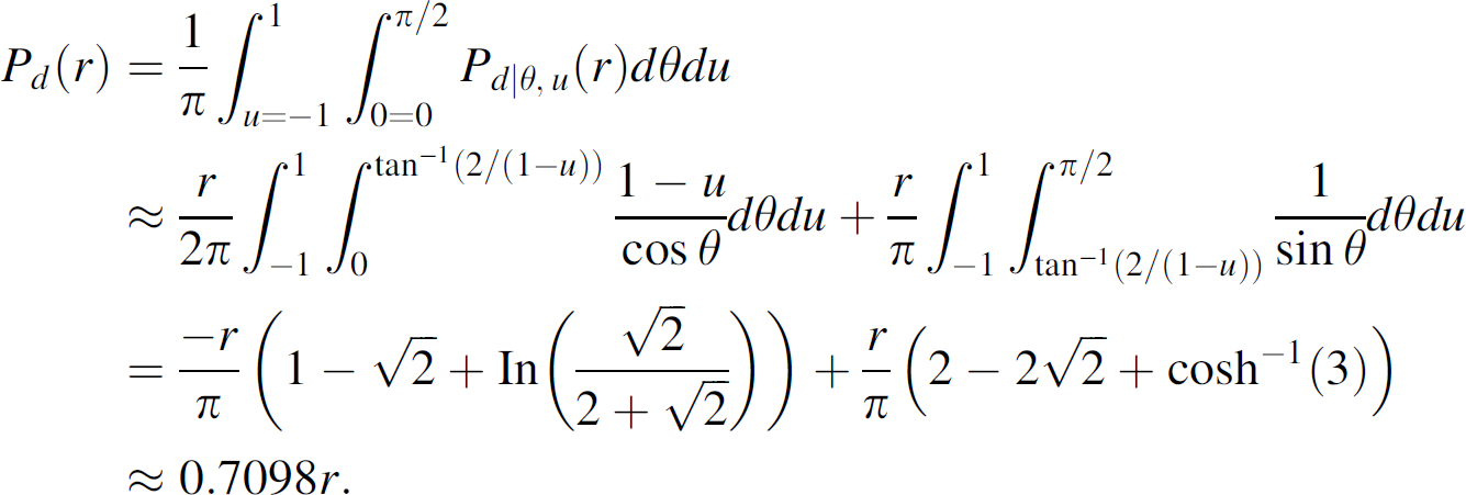
The rectangle-based approach yields an approximation for likelihood of detection that is linear in sensing radius r. (For general values of U, the approximation to probability of detection is given by $P_{d} (r) \approx 0.7098 r / U$ .)

To evaluate the accuracy of the analytically-derived approximation to the probability of detection, we simulate the likelihood of detection for a single sensor randomly placed in the sea base for values of r between 0 and 1 and compare the results to our approximation for 0 ≤ r ≤ 1. Figure 8 shows the approximate and empirical values of P_d(r) as a function of r. The linear approximation generated via analytical means provides results nearly identical to those generated empirically for values of r below approximately 0.75, or equivalently for sensors whose diameter is less than 75% of the length of one side of the square. In many detection scenarios, the size of the region to be monitored will be considerably larger than the sensing range of an individual sensor, even when sophisticated platform-based sensors are employed. Hence, we argue that the values of r of interest are those that are significantly less than U and thus the linear approximation to the probability of intersection can be employed with a minimal introduction of error.

Figure 8.

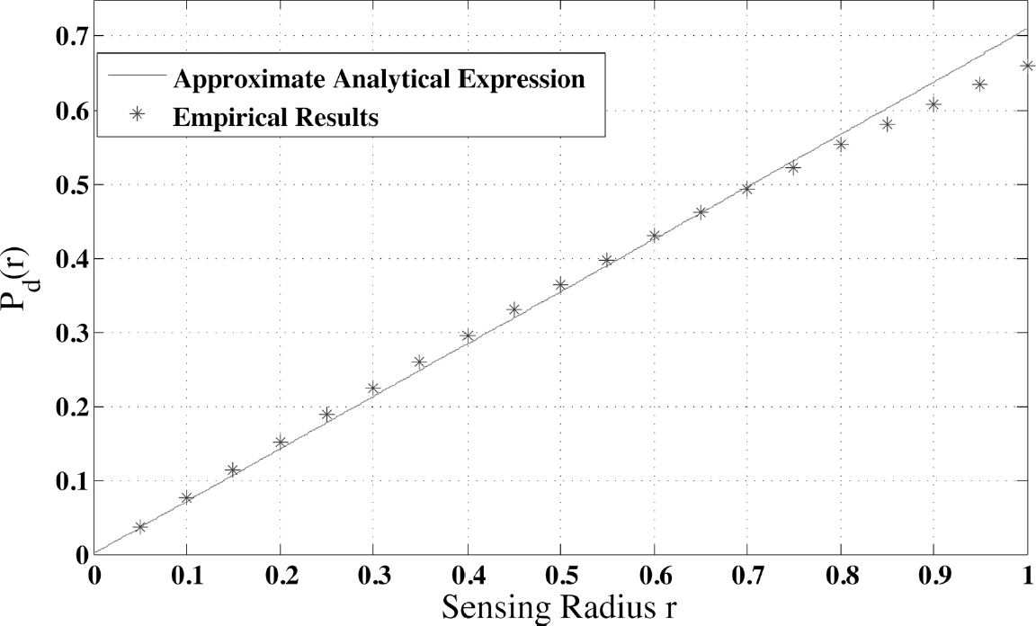
Probability that a straight-line target is detected by a single sensor with radius r and center randomly located within the sea base, U = 1. The approximate analytical expression is plotted as a solid line; stars denote empirical results for the same parameters.

Now consider a scenario in which, rather than having a known sensing radius r, the radius of the randomly-placed sensor is a stochastic variable drawn from the probability density function f(r). (We continue to assume U = 1 to simplify presentation.) The likelihood of detection in this case is given by

\begin{aligned} P_{d} & = \int_{0}^{\infty} P_{d} (r) f (r) d r \\ = 0.7098 \int_{0}^{\infty} r f (r) d r, \end{aligned}

(6)

where the second line is obtained using the linear approximation (5) to P_d(r). Hence, the detection probability for a random sensor network with heterogeneous sensing radius varies directly as the mean of the sensing radii. As we will see shortly, the detection probability also varies inversely as the area of the surveillance region. Thus, (6) may be written as

P_{d} \approx \frac{2.8392 \int_{0}^{\infty} r f (r) d r}{| | Ω | |},

(7)

where Ω is the surveillance region and ‖Ω‖ is its area. In our derivations and examples, we use Ω = [−1, 1] × [−1, 1], hence (in this case) the result reduces to (6).

For our work, we consider a system in which the sensor range to detection follows a beta-type density:

f (r) = \frac{Γ (α + β)}{Γ (α) Γ (β)} \frac{1}{c} (r / c)^{α - 1} (1 - r / c)^{β - 1}, r \in [0, c], α, β > 0,

where Γ denotes the Gamma function:

Γ (z) = \int_{0}^{\infty} t^{z - 1} e^{- t} d t

. Here, sensors have a maximum detection radius of c and a mean detection radius of

\int_{0}^{\infty} r f (r) d r = \frac{α c}{α + β}

. As the ratio of α to β increases,

\int_{0}^{\infty} r f (r) d r

approaches c, and randomly-drawn values of r are concentrated near the maximum sensing radius. The shape of three example beta-type density functions, each with a mean value

\int_{0}^{\infty} r f (r) d r = 0.1

, are shown in Fig. 9. The beta-type density allows us to investigate the case where some sensors perform better than others. From a manufacturing standpoint, sensors may be designed to achieve a particular sensing radius, but some will fall short of that design parameter in practice. A heterogeneous model employing a beta-type distribution allows us to model such variability in manufactured specifications. Additionally, sensor sensitivity may decay over time due to power reduction, physical degradation, etc. For example, the detection range may deteriorate as the battery discharges, or the battery life might be extended by actively adjusting (reducing) the detection range, or limiting when the sensor transmits or processes results. As an extention, the distribution from which sensor radii are drawn may change as a function of time, thereby allowing us to model the evolution of detection capabilities.

Figure 9.

Examples of beta-type density functions with varying parameters α, β, and c. The three examples have the same mean value: $\frac{α c}{α + β} = 0.1$ .

In Table 1, we compare the mean detection rate (obtained via 100,000 simulations) provided by a single randomly deployed sensor to the detection rate predicted by (6). Column one contains the predicted estimates. Columns two through four pertain to the detection rate for a homogeneous system, while columns five through seven pertain to a heterogeneous system with sensing radius drawn from a beta-type distribution. r₀ is the radius of all sensors from the homogeneous system. $c = r_{0} \frac{α + β}{α}$ is the maximum radius attained in the heterogeneous system. This value is used for c in order to keep the mean detection range for the heterogeneous system equal to that of the homogeneous system. The surveillance region Ω = [−1, 1] × [−1, 1]. For the homogeneous system, predicted and simulation detection propabilities differ by nomore than 2.7%. For the heterogeneous system, the maximum difference increases slightly to 4.67%.

Table 1

Comparison of single sensor detection capability for homogeneous and heterogeneous systems. For each row, P_d is the predicted probability that a single randomly placed sensor will detect a random (constant course) target moving through the surveillance region

		Comparison of Single Sensor Detection Estimates
	$P_{d} (f) = \frac{2.8392 \int_{0}^{\infty} r f (r) d r}{\| \| Ω \| \|}$
	$f_{Hom} = δ (r - r_{0})$			$f_{Het} = \frac{Γ (α + β)}{Γ (α) Γ (β)} \frac{1}{c} (r / c)^{α - 1} (1 - r / c)^{β - 1}, r \in [0, c] .$
P_d	r ₀	P _{Hom (Sim)}	% - Dif	c	P _{Het (Sim)}	% - Dif
.0355	.0500	.0351	−1.13	.0835	.0355	−.11
.0710	.0710	.0714	.65	.1670	.0731	2.94
.1065	.1500	.1074	.89	.2505	.1057	−.73
.1420	.2000	.1410	−.67	.3340	.1411	.63
.1774	.2500	.1759	−.90	.4175	.1734	−2.26
.2129	.3000	.2073	−2.66	.5010	.2090	−1.84
.2484	.3500	.2446	−1.53	.5845	.2441	−1.74
.2839	.4000	.2785	−1.92	.6680	.2761	−2.77
.3194	.4500	.3128	−2.07	.7515	.3090	−3.27
.3549	.5000	.3453	−2.69	.8350	.3384	−4.66

Table 2 compares the predicted detection rate, P_D, of a randomly distributed sensor field to the estimate obtained via averaging over 10,000 simulations. For simulations of up to 40 sensors, the sensors are randomly deployed over the surveillance region. For more than 40 sensors, an equivalent (relative to surveillance region size) number of sensors were randomly distributed over a slightly larger surveillance space ([−1.05, 1.05] × [−1.05, 1.05]) to adjust for increased sensor detection area outside the surveillance region. Detection is still based on targets entering the original surveillance region; however, the coverage lost due to sensor coverage extending beyond the original surveillance region is counter-balanced by the coverage of the extra sensors that intrude into the surveillance region. Determining how much to increase the surveillance region is, at best, an art and needs further study.

Table 2

Comparison of predicted and actual detection rate for a sensor field consisting of N randomly distributed sensors. The sensor radii are randomly drawn from a beta-type density with parameters α = 1, β = 0.67 and c = 0.0167. The mean detection values, M_D, were obtained by averaging the detection rate for 10,000 network field simulations

	Sensor Field Detection Comparison
No. Sensors	Predicted Detection (P_D)	Mean Detection (M_D)	% - Error
N	$P_{D} = 1 - (1 - P_{d})^{N}$	M_D = Mean Coverage	$(M_{D} - P_{D}) / P_{D} \times 100$
1	.0071	.0075	5.60
5	.0350	.0345	−1.43
10	.0688	.0668	−2.91
20	.1328	.1298	−2.26
30	.1924	.1944	1.04
40	.2479	.2485	0.24
50	.2996	.3084	2.94
60	.3478	.3590	3.22
70	.3926	.3967	1.04
80	.4344	.4349	0.12
90	.4733	.4730	−0.06
100	.5095	.5012	−1.63

4.2. Extension of Analysis to General Convex Regions

Regions other than a square sea base may be of interest in detection applications. They include those defined as convex, i.e., regions for which any line segment drawn from one point on the closed perimeter to another remains inside the space. When a rectangular approximation is made to the detection region for a particular target path, the probability of detection for that path is dependent only upon the length of the path within the sea base and the mean sensing radius. Each path through the sea base is a chord in the convex region. Since the sensing radius r and the chord length c are independent random variables, the average area of a rectangular detection region can be expressed as $| | \tilde{A} | | = 2 \overset{ˉ}{c} \int_{0}^{\infty} r f (r) d r$ where $\overset{ˉ}{c}$ denotes the mean chord length for the convex region of interest. The detection probability is then approximated by the ratio of the mean detection region area to the total area:

P_{d} \approx \frac{2 \overset{ˉ}{c} \int_{0}^{\infty} r f (r) d r}{| | Ω | |},

where ‖Ω‖ denotes the area of the surveillance region Ω.

5. Contrasting Detection and Coverage

In designing or evaluating sensor networks for surveillance applications, coverage of the region by the sensor network is often chosen as a performance metric [12, 16–18]. In other words, what fraction of the region of interest lies within the detection region of at least one (or perhaps at least k) sensors? While a relationship undoubtedly exists between coverage and detection capabilities, our analysis shows that when the goal of the network is to detect intruders traveling a straight path through the sea base, the fraction of the region covered by the network of sensors underestimates the probability of detection. Additionally, under our assumptions, a given coverage provided by a single large sensor does not necessarily yield the same P_d as a set of smaller sensors with the same cumulative coverage area.

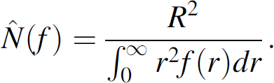
To better understand this phenomenon, recall from (1) that the coverage provided by a network of sensors is given by $ρ = 1 - \exp {- λ π \int_{0}^{\infty} r^{2} f (r) d r}$ , where λ is the mean number of sensors per unit volume. Thus, the average number of sensors deployed over ‖Ω‖ is $N (f) = λ | | Ω | |$ . Therefore, on average, the number of smaller sensors required for the randomly deployed network to have the same coverage as a single large sensor (of sensor radius R) placed at the center of the surveillance region satisfies

1 - e^{- \frac{π N (f)}{| | Ω | |} \int_{0}^{\infty} r^{2} f (r) d r} = \frac{π R^{2}}{| | Ω | |} .

Solving for $N (f)$ ), we obtain the average number of randomly-deployed smaller sensors required to achieve the same coverage as a single large sensor:

N (f) = \frac{- | | Ω | | \log (1 - \frac{π R^{2}}{| | Ω | |})}{π \int_{0}^{\infty} r^{2} f (r) d r} .

(8)

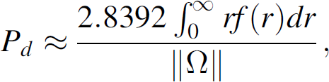
Using L'Hôpital's rule, one can show that, as the surveillance region grows large, i.e., in the limit as ‖Ω‖ approaches ∞, (8) becomes

\hat{N} (f) = \frac{R^{2}}{\int_{0}^{\infty} r^{2} f (r) d r} .

(9)

For the special case in which the system of small sensors have identical sensitivity range r₀, $\hat{N} (δ (r - r_{0})) = R^{2} / r_{0}^{2}$ . Expression (9) holds in the important case in which the surveillance region is large relative to the number and size of sensors in use and there is little chance of the randomly deployed sensors having regions of overlapping coverage.

Figure 10 shows the number of smaller sensors required to achieve the same coverage as a single centered sensor with radius R. The number of small sensors required is plotted as a function of their mean sensing range. Both fixed sensing range and sensing range drawn from a beta-type distribution are considered. As the mean sensing radius decreases, the number of sensors required to achieve a particular coverage level increases exponentially. This can be attributed to two factors. First, the coverage area scales with the square of the sensing radius. Second, as the number of sensors deployed increases, the likelihood that the sensing regions overlap also increases, and hence additional sensors contribute less on average to the total sensing area.

Figure 10.

Number of small sensors required to achieve the same coverage as a single sensor (centered at the origin) with radius R = 1. Mean sensing range for the small sensors varies as the horizontal axis. Results for fixed small sensor radius are shown with a plus, and the results for small sensing radius drawn from a beta-type distribution are shown with a circle.

In contrast, the presence of the sensing area overlap does not pose the same detriment to detection capabilities. Figure 11 compares the detection performance of a single large sensor to two systems of smaller homogeneous sensors, one in which the sensing radius is r₀ = 0.05, and one in which the sensing radius is r₁ = 0.2. The sea base is assumed to have area 4 square units, e.g., U = 1. The cumulative coverage of the random systems are adjusted so that they equal the total coverage of the single sensor. For example, $P_{d}^{(c)} (R)$ , detection probability for a single sensor with sensing radius R, is compared to $P_{d}^{(M)} (r)$ for M sensors with $r = R / \sqrt{M}$ . Note that the sensing areas of the M smaller sensors may overlap, and hence the total coverage provided by the M sensors may be smaller than that provided by the single large sensor. One can quickly glean that, despite the possibility for overlap, the detection performance improves as the number of sensors increases while the total sensing area is held constant.

Figure 11.

Likelihood of detection as a function of cumulative sensing area for homogeneous sensor fields with varying detection ranges. A single sensor with radius R and sensing area (or equivalently coverage) πR² is compared to a field of M₀ = 400A/π sensors of radius r₀ = 0.05 and a field of M₁ = 25A/π sensors of radius r₁ = 0.2. The seabase is given by Ω = [−1, 1] × [−1, 1]. For fixed cumulative sensing area, probability of detection increases as individual sensing range decreases.

Let $M (f)$ denote the number of small sensors (with range sensitivity density f(r)) needed to achieve a detection probability of at least P_d(R), where P_d(R) denotes the detection probability for a single centered sensor with radius R and is given by (2). That is, $M (f)$ ) is the smallest value of M satisfying

1 - [1 - P_{d}]^{M} \geq P_{d} (R),

(10)

where the left side of (10) is the probability of detection by at least one of M sensors with radii distributed according to f(r). Solving for M(f), we obtain

\begin{aligned} M (f) & \geq \frac{\log [1 - P_{d} (R)]}{\log [1 - P_{d}]} \\ \approx \frac{\log [1 - P_{d} (R)]}{\log (1 - \frac{2.8392 \int_{0}^{\infty} r f (r) d r}{∥ Ω ∥})} . \end{aligned}

(11)

Table 3 compares the number of smaller sensors required to achieve the same coverage as a single sensor (centered at the origin) with R = 0.75 to the number of smaller sensors required to obtain the same detection probability as the single large sensor - both as a function of the sensing radii of the smaller sensors. Clearly, the number of sensors required to provide equivalent detection is significantly less than that required to provide equivalent coverage, and the magnitude of the difference increases as the sensing radii of the smaller sensors decrease. For example, for r = 0.10, detection requires approximately 12% (9 versus 74) of the sensors required for coverage. For r = 0.01, the detection requires only 1.2% (87 versus 7423) of the sensors required for coverage. Put briefly, increasing the detection probability requires significantly fewer sensors than increasing the expected coverage. A quick look at (8) and (11) reveals that while coverage scales with the square of the sensing radius, detection probability is approximately linear in sensing radius. One can consider this in the framework of comparison to a single large sensor.

Table 3

Comparison of the number, N_f, of small random sensors required to achieve the same coverage probability as a single large sensor centered at the origin, and the number, $M_{f}^{(k)}$ , of small random sensors required so that the probability of detection (by at least k sensors) is at least as great as detection probability for a single large sensor centered at the origin. Surveillance region Ω = [−1, 1] × [−1, 1]

Comparison of Sensor Requirements for Coverage and Detection
	Single Sensor
	R = 0.75			$P_{d}^{(c)} (R) = 0.462$
Multiple Sensors
$M_{f}^{(k)} = min_{M} {1 - \sum_{i = 0}^{k - 1} (\binom{M}{i}) (1 - P_{d})^{M - i} P_{d}^{i} \geq P_{d}^{(c)} (R)}$
r	N_f	$M_{f}^{(1)}$	$M_{f}^{(2)}$	$M_{f}^{(3)}$	$M_{f}^{(4)}$	$M_{f}^{(5)}$
.400	5	2	6	9	13	16
.200	19	5	11	18	25	32
.150	33	6	15	24	33	42
.100	74	9	22	36	49	63
.080	116	11	28	45	62	79
.060	206	15	37	59	82	105
.040	464	22	55	89	123	158
.030	825	29	73	119	164	210
.020	1856	44	110	178	246	315
.010	7423	87	220	356	492	630

6. Discussions and Conclusion

We have developed a framework for analytically approximating the detection capabilities of a randomly-deployed heterogeneous sensor field. Using this framework, we have derived an approximation to probability of detection that is a function of only the number of sensors deployed and the mean sensing radius. Empirical results confirm that our approximation yields very good results, with, in general, a small margin of error. The approximation provides a valuable tool for time-constrained decision making, as one can instantly estimate the necessary network size to achieve a desired detection performance without the need for any simulation or in-depth analysis. Additionally, we have shown how, using results from integral geometry, the simple approximation to P_d that we have derived for a square region of interest can be easily extended to any convex surveillance region.

We have directly compared the coverage and detection capabilities of randomly-distributed heterogeneous sensors and have shown that, while the number of sensors required to achieve a given coverage level increases exponentially as the desired coverage level increases, the number of sensors required to achieve a desired detection probability increases much more slowly. These results are fundamental to the analysis of randomly-deployed sensor networks for surveillance applications, as they imply that, when detection of a moving target is the goal, coverage is not the metric that best indicates performance, and in fact, coverage greatly overestimates the network size required to achieve a particular probability of detection. The modest number of sensors required to achieve high detection probability in a heterogeneous sensor field, as well as the sensor field's ability to achieve higher detection probability than a single sensor for the same cumulative sensing area, holds strong promise for randomly-distributed sensor networks as a practical approach to surveillance at a more reasonable cost than traditional coverage-based analysis would suggest. Building on the framework developed here, future work will consider the tracking capabilities of the sensor field and the communication requirements for cooperative detection and tracking.

References

Wong

K. D.

Y. H.

Sayeed

A. M.

, “Detection, classification, and tracking of targets,” IEEE Signal Processing Magazine, vol. 19, no. 2, pp. 17–29, March 2002.

Chamberland

J. -F.

Veeravalli

V. V.

, “Wireless sensors in distributed detection applications,” IEEE Signal Processing Magazine, vol. 24, no. 3, pp. 16–25, 2007.

National Research Council, Distributed Remote Sensing for Naval Undersea Warfare, The National Academies Press, Washington, D.C., 2007.

Onur

Ersoy

Delic

, “Analysis of target detection probability in randomly deployed sensor networks,” IEEE Communications Letters, vol. 11, no. 10, October 2007.

Megerian

Koushanfar

Potkonjak

Srivastava

M. B.

, “Worst and best-case coverage in sensor networks,” IEEE Transactions on Mobile Computing, vol. 4, no. 1, pp. 84–92, January/February 2005.

Mehta

D. P.

Lopez

M. A.

Lin

, “Optimal coverage paths in ad-hoc sensor networks,” in Proceedings of the IEEE International Conference on Communications, May 2003, pp. 507–511.

Ram

S. S.

Manjunath

Iyer

S. K.

Yogeshwaran

, “On the path coverage properties of random sensor networks,” IEEE Transactions on Mobile Computing, vol. 6, no. 5, May 2007.

Liu

Towsley

, “A study of the coverage of large-scale sensor networks,” in IEEE International Conference on Mobile Ad-hoc and Sensor Systems, October 2004, pp. 475–483.

Clouqueur

Phipatanasuphorn

Ramanathan

Saluja

K. K.

, “Sensor deployment strategy for detection of targets traversing a region,” Mobile Networks and Applications, pp. 453–461, August 2003.

10.

Cox

, “Cumulative detection probabilities for a randomly moving source in a sparse field of sensors,” in Proceedings of the Twenty-Third Asilomar Conference on Signals, Systems, and Computers, October 1989, vol. 1, pp. 384–389.

11.

Traweek

C. M.

Wettergren

T. A.

, “Efficient sensor characteristic selection for cost-effective distributed sensor networks,” IEEE Journal of Oceanic Engineering, vol. 31, no. 2, pp. 480–486, April 2006.

12.

Rowe

E. G.

Wettergren

T. A.

, “Coverage and reliability of randomly distributed sensor systems with heterogeneous detection range,” International Journal on Distributed Sensor Networks, 2008, to appear.

13.

Sakkottai

Srikant

Shroff

, “Unreliable sensor grids: Coverage, connectivity, and diameter,” in Proceedings of IEEE Infocom, 2003.

14.

Hall

Peter

, Introduction to the Theory of Coverage Processes, John Wiley and Sons, New York, 1988.

15.

Karlin

Taylor

H. M.

, A Second Course in Stochastic Processes, Academic Press, San Diego, CA, 1981.

16.

Ahmed

Kanhere

S. S.

Jha

, “Probabilistic coverage in wireless sensor networks,” in Proceedings of the IEEE Conference on Local Computer Networks, 2005.

17.

Dhillon

S. S.

Chakrabarty

, “Sensor placement for effective coverage and surveillance in distributed sensor networks,” in Proceedings of IEEE Wireless Communications and Networking, March 2003, pp. 1609–1614.

18.

Adlakha

Srivastava

, “Critical density thresholds for coverage in wireless sensor networks,” in Proceedings of IEEE Wireless Communications and Networking, March 2003, pp. 1615–1620.

Detection Capabilities of Randomly-Deployed Sensor Fields

Abstract

Keywords

1. Introduction

2. System Model

4.1. Detection Probability for a Single Sensor

5. Contrasting Detection and Coverage

References