Sage Journals: Discover world-class research

Abstract

We consider a network of randomly-deployed, low-cost sensors and a single powerful sink node. A partition-based localization algorithm is proposed in which the sink node imparts sector-based location information through the phased-array transmission of a series of beacons. One-hop neighbor information is used by each sensor in a series of sector-partitioning routines to identify the sub-sector in which it resides. A geographic routing algorithm is then proposed which uses the sector-based localization results as the basis for a routing algorithm. Simulation results indicate that the performance of our localization algorithm improves with node density, and that the performance of the combined localization and routing algorithm in the presence of severe measurement noise is comparable with that provided by the same routing algorithm using perfect location information.

Keywords

Partition-based Localization Geographical Routing Energy-preserving Distributed Algorithm Wireless Sensor Networks

1. Introduction

Location information is critical for many wireless sensor networking applications, including habitat monitoring, critical infrastructure protection, and target tracking. In addition, location information also plays a significant role in some energy-preserving routing protocols designed for wireless sensor networks, such as SELAR [1] by Lukachan. However, location awareness often comes at the cost of pre-deployment planning or the use of GPS or similar relatively expensive technologies, which may not be practical for networks intended for rapid deployment and composed of a large number of low-cost sensor nodes.

Most localization methods in the literature assume the existence of several location-aware nodes called anchors (also called beacons or reference points), whose positions are obtained via GPS or manual configuration, so as to enable all the nodes in the network to find their absolute geographical positions. These schemes are categorized as anchor-based localization methods.

The place where the location estimation computation is performed provides an added basis for discrimination, providing the subcategories of centralized and distributed localization methods. Centralized localization methods depend on sensor nodes transmitting data to a central base station that performs location estimation computation based on collected global knowledge. The central base station then broadcasts the results. The “convex optimization” method proposed by Doherty [2] is an example; this reference describes the construction of a bounding box for a node by considering the intersection of all its neighboring nodes' communication ranges. The centroid of this box is the estimated position of the node. Since centralized methods would always have heavy traffic load for high density networks and therefore be less scalable, they are generally not preferred by high density/large scale wireless sensor networks. Instead, distributed localization methods are suggested, where each node performs location estimation from its knowledge of anchor locations and communication links.

Based on the type of knowledge used, the distributed anchor-based methods can also be divided into two sub-categories: distance-free and distance-aware approaches. An example of the former is the “Centroid” method proposed by Buluse [3], which is based on connectivity information and lets each unknown node set its location to the centroid of its neighboring anchors. The localization accuracy is about one-third of the separation distance between anchors, requiring high anchor density for peak performance. The APIT method proposed by He [4] is another distance-free method, in which a node first identifies all the triangles formed by audible anchors, and then calculates the center of gravity of the intersection of all these triangles to determine its estimated position. This algorithm is distance-free in that only the monotonically decreasing relationship between signal strength and physical distance is used, while there is no quantitative mapping between the signal strength measurements and the physical distances. The APIT method has been shown to perform well even under irregular radio patterns and random node placement; however, in a real deployment, calibration issues may arise due to the significance placed on the RSS value read by different sensor nodes while performing APIT test. The APS methods proposed by Niculescu and Nath [5] use both distance-free and distance-aware approaches to obtain distance estimates to anchors. In their DV-hop method, each node finds its distance estimate to an anchor based on the hop counts of the shortest connecting path; while in their DV-distance method, each node sets its distance estimate to an anchor as the total length of all the links in its shortest connecting path. DV-hop is less sensitive to measurement noise, but has poorer performance compared with DV-distance under moderate measurement noise.

Anchor-based localization methods often require that the anchors have appropriate density and distribution to ensure satisfying localization accuracy, which limits their application in real wireless sensor network scenarios. The KPS scheme proposed by Lei [6] removes the dependence on anchors, and models the location discovery problem as a statistical estimation problem. The maximum likelihood estimation method is used based on the knowledge of deployment points' location and the prior knowledge of sensor nodes' probability distribution function, which results in location estimation accuracy sufficient to support various applications. However, its strong dependence on the distribution of the nodes limits its application to static wireless sensor networks; in addition, accurate deployment knowledge is hard (or expensive) to insure in practice.

With the assumption that location information is always available in a wireless sensor network — either directly from pre-deployment knowledge, or indirectly from the localization process, geographic routing algorithms have been suggested for such networks. They have the goal of minimizing storage, since they only require direct neighbors' location information; they are also expected to conserve energy as well as bandwidth, since discovery floods and state propagation are not required beyond one hop.

There have been quite a few geographic routing protocols proposed for wireless ad hoc networks, as evidenced by [7] [8] [9] [10] [11] [12] [13] [14]. Since wireless sensor networks require less mobility considerations and have more strict energy constraints compared with wireless ad hoc networks, the design of geographic routing protocols for the former has some unique considerations.

SELAR [1] is a scalable energy-efficient geographic routing protocol proposed for wireless sensor networks, which utilizes the location and energy information of neighboring nodes as well as the location information of the sink node to perform the routing function. SELAR outperforms flooding in terms of network lifetime, energy distribution, and the amount of data delivered. In [15] the authors showed that location errors could yield poor performance or even complete failure in reality for geographic routing protocols that assume the existence of exact position information, and provided fixes for them to improve the delivery ratio as well as save energy in case of location errors.

Although the research on localization algorithms and geographic routing protocols for wireless sensor networks has been extensive, to the best of our knowledge these two research topics have been studied separately, and the consideration of these two as – twin sides of a more general problem of deployment is novel. However, it should be noted that localization and geographic routing algorithms are tightly coupled - the localization process provides the location information that is the fundamental element for geographic routing. If satisfying routing performance could be achieved with imperfect location information, then we can save the cost spent in increasing localization accuracy without reducing the network's performance. Intuitively, this could be achieved if the localization and routing algorithms are designed in such a way that most of the location estimation errors do not affect routing performance. Thus we argue in this paper that high-performance, low-cost localization, and geographic routing can be achieved through co-design by proposing a combined localization and geographic routing algorithm and studying their joint performance.

We focus in this paper on wireless sensor networks consisting of a single sink node at the center of a field of randomly distributed sensors. We first present a partition-based lightweight localization algorithm, which is both distributed and anchor-free, and uses a series of beacons generated by the sink as well as localized peer-to-peer transmissions as the basis for sensor localization. Then we propose a geographic routing algorithm designed to be used in combination with this partition-based localization algorithm, which effectively avoids the location estimation errors' impacts and achieves high energy efficiency. The performance of our combined algorithm is compared with that of the same geographic routing algorithm utilizing perfect location information by simulations to show the effectiveness of co-design.

Section II of this paper lists network assumptions made in our research. Section III describes our partition-based localization algorithm in detail. Section IV introduces performance metrics for this algorithm, and provides simulation results of its performance evaluated using these metrics. Section V describes the geographic routing algorithm. Section VI shows the effectiveness of our combined localization and geographic routing algorithm by simulations. Section VII provides comments on this research.

2. Network Assumptions

Consider a circular coverage area with radius R and a data sink (base station, BS) at its center. During deployment, N sensor nodes with the same adjustable transmission power are randomly distributed in the circular area (without prior planning), creating a 2-D uniform distribution (high-density) of sensor nodes.

The BS uses phased array antennas to broadcast M beacons with limited beam width, each beacon associated with an angular range in the coverage area. The beacons thus equally divide the circular coverage area into M beacon sectors. The beacon broadcasts are scheduled in sequential time slots and distinguished by beacon sector numbers included in the transmission. All of the nodes in the network are time-synchronized at deployment. After the transmission of all directional beacons, the BS broadcasts strong omnidirectional signals which enable all the nodes to estimate their distance to the data sink using Time of Arrival (TOA) technique. Thus, each node gets its initial coarse location information in the form of current sector number and estimated distance to the data sink after the BS's directional and omnidirectional broadcasts. The TOA measurements might be noisy which would make the distance estimates inaccurate; and the initial beacon sector information also might be erroneous especially for nodes on the sector borders. However, the existence of these error sources will only slightly deteriorate our localization as well as geographic routing algorithm's performance, as we will show later in the simulation sections.

For static sensor networks, all the nodes can build up initial coarse location information right after the BS's broadcasts and thus get prepared for the partition-based localization process. Node mobility can be adapted when it has negligible impact on the 2-D uniform distribution assumption, either through the BS's periodic broadcasts, or by triggering the BS's broadcasts whenever there is a need with the help of localized neighbors. However, in this paper we only focus on static networks, the study of which could provide a performance baseline. More discussions on handling the mobility scenarios would be our future work.

3. Partition-Based Localization Algorithm

Since we consider high-density wireless sensor networks in this paper, distributed algorithms are preferred. Thus our localization algorithm is designed to be executed parallely at each unknown node, and only information of its one-hop neighbors is used for a node's location estimation. The essential of our localization algorithm is partition-based, in that each node keeps equally partitioning its current sector into two sub-sectors, and deciding which sub-sector it exists in based on neighbor information till accuracy requirement controlled by some parameter is satisfied. This localization algorithm is based on the one published in [16], with revisions for better localization performance and subsequent geographic routing algorithm's convenience.

Partition decisions are made at each unknown node utilizing merely its neighbor list, which is built up by broadcasting MSG messages containing the following data elements:

node number i

estimated distance to the BS r_i

current sub-sector number m_i

current view of the total number of sectors M_i

localization completion flag f_i

estimated angle φ_i

energy level indicator l_i

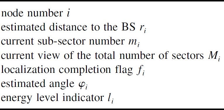
After receiving the BS's directional and omnidirectional broadcasts, each node i sets its r_i using the TOA measurement, sets its current sub-sector number m_i to the beacon sector number received, and sets its current view of the total number of sectors M_i to M. The localization completion flag f_i indicates whether additional partition rounds are needed for node i, and is set to 1 for all the nodes before the localization process. The estimated angle is updated after each partition round and is used only when f_i is not 1, and the energy level indicator l_i is designed for the subsequent energy-aware routing algorithm and will be introduced later.

The MSG message broadcasts follow two simple rules: firstly, all nodes send MSG using full transmission power after deployment and receiving the BS's broadcasts; secondly, each node broadcasts an updated MSG using full transmission power if its content does change whenever a partition round ends.

Whenever a node receives a MSG from some one-hop neighbor for the first time, it makes an entry for this neighbor in its neighbor list. The entry is simply the data elements in the received MSG of that neighbor plus the distance to that neighbor estimated using RSS. The entries are updated as new MSG messages are received, and therefore kept up to date for partition use.

The flow chart in Fig. 1 is the detailed description of our partition-based localization algorithm carried out at each node i.

Figure 1.

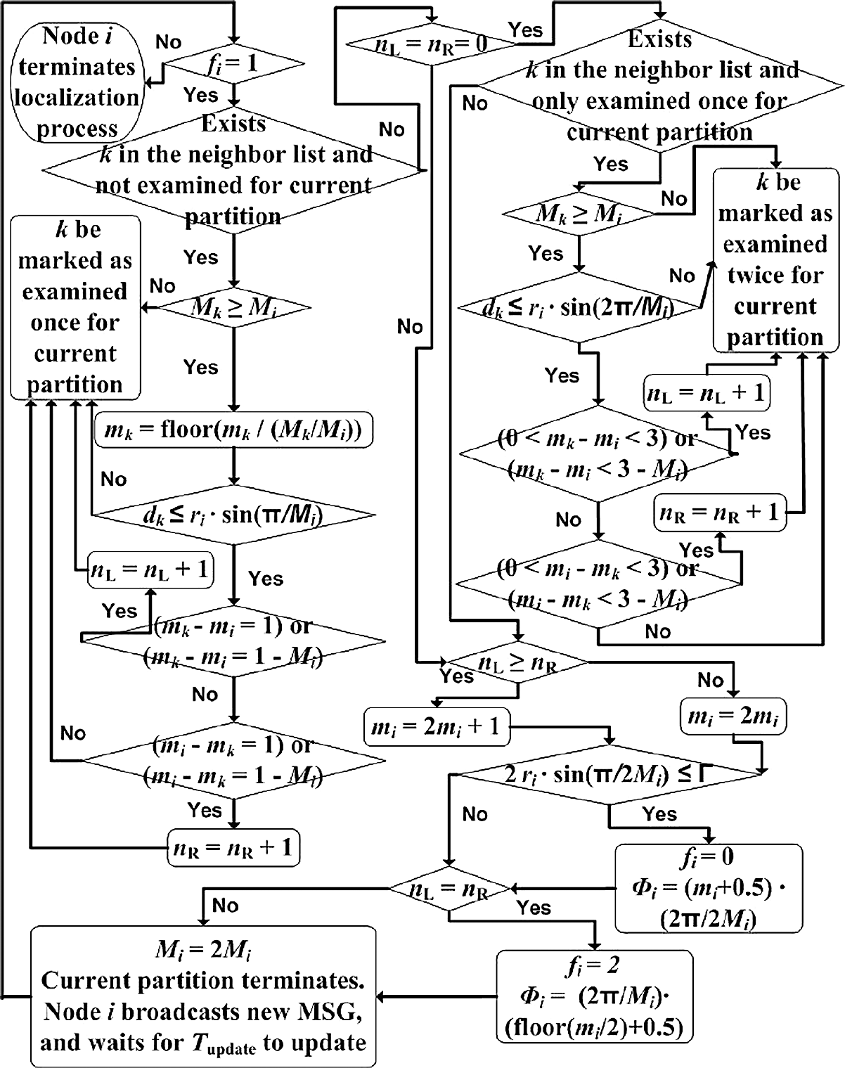
Flow chart of the partition-based localization algorithm.

As is shown in the flow chart, during the localization process, each node i waits for T_update to update entries for all its neighbors before starting a further partitioning round. Then it traverses its neighbor list, applying the checking conditions on each entry and increasing its number of left neighbors (n_L) or number of right neighbors (n_R) accordingly. After checking all the entries, it determines itself to be in the left (larger angle) sub-sector if n_L ≥ n_R, or in the right (smaller angle) sub-sector if n_L < n_R. In addition, if n_L = n_R, it announces itself to be on the common edge of these two sub-sectors (middle line of the parent-sector) and terminates localization by setting f_i to 2. Otherwise, if it finds itself in a sub-sector with maximal location inaccuracy no larger than the preset threshold parameter Γ, it announces itself to be on the middle line of the current sub-sector and terminates localization by setting f_i to 0.

The checking conditions listed in the algorithm flow chart include the comparison of node i and its neighbor k's current views of the total number of sectors (M_i and M_k), and here is some explanations. At the beginning of the localization algorithm, we have M_i = M_k for any node pair i and k, since this value is set to M for each node after the BS's beacon broadcasts. However, since M_i is doubled after each partition round at node i, nodes would have different M_i's depending on how many partition rounds have been carried out before its localization process is terminated. For any node i, a neighbor k with M_k < M_i will not be used in left/ right neighbor counting, since its m_k is of lower granularity and does not tell whether it is node i's left or right neighbor; while a neighbor k with M_k > M_i can be used by reducing m_k to the same granularity as m_i as shown in the flow chart. The situation of having a neighbor k with smaller M_k would arise when node k has completed its localization process in less partition rounds and stopped doubling its M_k earlier than node i, or the updated MSG sent from node k was not successfully received at node i. The situation of having a neighbor k with M_k > M_i would happen if node i is a mobile node, and its localization process starts after all other neighbors have completed localization, in which case the same MSG message from a neighbor is used during each partition round with appropriate granularity adjustments.

As an algorithm improvement compared with the one published in [16], each node first inspects a smaller neighbor region for left / right neighbors, and then enlarges this small neighbor region if the numbers of left and right neighbors in this region are both zero. This not only reduces the number of wrong “on the middle line” decisions, but successfully reduces the number of wrong left/ right sub-sector decisions, thus improves the localization performance as we will see in the next section.

4. Analysis of the Localization Algorithm

4.1. Performance Metrics

After the partition-based localization process is completed, each node is provided with two forms of location information: the sector-based location information and the angle-based location information, where the latter is obtained by setting a node to the middle-line of its final sub-sector, and is used for the evaluation of the localization performance as follows. We define a node's location inaccuracy as the distance between its estimated angle-based location and its actual location, and then define our algorithm's localization inaccuracy as the average of all the nodes' location inaccuracies. We announce a localization error if a node's location inaccuracy exceeds the preset threshold parameter Γ of maximal allowed location inaccuracy, and then define the localization error rate as the ratio of the number of localization errors over the number of nodes in the circular network area.

The former, although not an exact position, turns out to be critical for our joint localization and routing algorithm design, and also provides some important performance metrics for our localization algorithm, as we will explain below.

d_{i j min} = {\begin{cases} \sqrt{r_{1 max}^{2} + r_{2 min}^{2} - 2 \cdot r_{1 max} \cdot r_{2 min} \cdot cos α_{i j min}} & : r_{1} < r_{2 min} \cdot cos α_{i j min} \\ \sqrt{r_{1 min}^{2} + r_{2 min}^{2} - 2 \cdot r_{1 min} \cdot r_{2 min} \cdot cos α_{i j min}} & : r_{2 min} \cdot cos α_{i j min} \leq r_{1} < r_{2 min} - Δ r \\ 2 \cdot r_{2 min} \cdot sin \frac{α_{i j min}}{2} & : r_{1} \geq r_{2 min} - Δ r \end{cases}

(1)

d_{i j max} - {\begin{cases} \sqrt{r_{1 min}^{2} + r_{2 max}^{2} - 2 \cdot r_{1 min} \cdot r_{2 max} \cdot cos α_{i j max}} & : r_{1} < r_{2 max} \cdot cos α_{i j max} \\ \sqrt{r_{1 max}^{2} + r_{2 max}^{2} - 2 \cdot r_{1 max} \cdot r_{2 max} \cdot cos α_{i j max}} & : r_{1} \geq r_{2 max} \cdot cos α_{i j max} \end{cases}

(2)

In the data communication phase, a node chooses the required transmission power to the next relay node according to the distance between them. This distance can be obtained by mapping from the RSS measurement, which would be a value varying around the actual distance; it can also be obtained by computing from these two nodes' estimated locations, which would also include some inaccuracy. Therefore, no matter which method is used, the distance obtained is not accurate, and to ensure successful reception, a node would use d + Δd instead of the obtained distance d in selecting the transmission power. The selection of Δd therefore represents the preference between ensuring successful reception and reducing energy consumption, and it is not easy to find a guideline for choosing Δd. Our partition-based localization algorithm instead provides specific information regarding to the choice of Δd, because it enables finding the maximal possible distances between any two one-hop neighbors.

Since the TOA measurements might be noisy in real applications, we assume the actual distance between the BS and a node i with estimated distance r_i to be in the range [r_imin, r_imax], where r_imin = max(0, r_i − Δ₁), r_imax = min(R, r_i + Δ₁), and Δ₁ can be set to 0 for perfect TOA measurements. Thus after the partition-based localization process is completed, it is reasonable to assume node i in a fan-shaped area with r_i ∊ [r_imin, r_imax], and θ_i ∊ [θ_imin, θ_imax], where

\begin{aligned} θ_{i min} & = {\begin{cases} m_{i} \cdot \frac{2 π}{M_{i}} & : f_{i} = 0 \\ (⌊ \frac{m_{i}}{2} ⌋ + \frac{3}{4}) \cdot \frac{2 π}{M_{i} / 2} & : f_{i} = 2 \end{cases} \\ θ_{i max} & = {\begin{cases} (m_{i} + 1) \cdot \frac{2 π}{M_{i}} & : f_{i} = 0 \\ (⌊ \frac{m_{i}}{2} ⌋ + \frac{3}{4}) \cdot \frac{2 π}{M_{i} / 2} & : f_{i} = 2 \end{cases} \end{aligned}

Thus the angle α_ij between two arbitrary nodes i and j would be in the range [α_ijmin, α_ijmax]. Without loss of generality, we assume θ_imax ≥ θ_jmax, and determine α_ijmin, α_ijmax as follows:

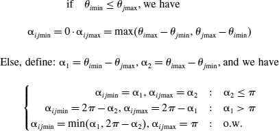
\begin{aligned} if θ_{i min} \leq θ_{j max}, we have \\ α_{i j min} = 0 \cdot α_{i j max} = max (θ_{i max} - θ_{j min}, θ_{j max} - θ_{i min}) \\ Else, define : α_{1} = θ_{i min} - θ_{j max}, α_{2} = θ_{i max} - θ_{j min}, and we have \\ {\begin{cases} α_{i j min} = α_{1}, α_{i j max} = α_{2} & : α_{2} \leq π \\ α_{i j min} = 2 π - α_{2}, α_{i j max} = 2 π - α_{1} & : α_{1} > π \\ α_{i j min} = min (α_{1}, 2 π - α_{2}), α_{i j max} = π & : o . w . \end{cases} \end{aligned}

It is reasonable to assume that a power efficient routing protocol will never let a node i relay to a neighbor j with $α_{i j min} \geq \frac{π}{2}$ . Let r₁ = min(r_i, r_j), r₂ = max(r_i, r_j), then the distance d_ij between node i and its one-hop neighbor j can be bounded in the range [d_ijmin, d_ijmax] as defined in (1) and (2).

Therefore, each node i can estimate its minimal and maximal possible distance to each neighbor node j from the entries of its neighbor list. The estimated d_ijmin and d_ijmax are added into the corresponding entries of node i's neighbor list for subsequent routing use.

Since for wireless communications, the received signal power at distance d has mean value ${\bar{P}}_{r} (d) = P_{0} \cdot (\frac{d}{d_{0}})^{- n}$ , given that the transmitted signal power at distance d₀ is P₀, where N is the path-loss exponent typically taking integer values between 2 and 4. Thus in the communication phase, if we define the power threshold for successful reception as Γ_P, with the sector-based location information provided by our partition-based localization process, each node i can use power $P_{i j} = Γ_{P} \cdot (\frac{d_{i j max}}{d_{0}})^{n}$ to ensure successful reception at neighbor j. While the minimal power required for successful reception is $P_{i j min} = Γ_{P} \cdot (\frac{d_{i j}}{d_{0}})^{n}$ , where d_ij is the actual distance between node i and node j. It is clear that the closer d_ijmax to d_ij, the less energy is wasted in transmission, and thus d_ijmax affects the energy efficiency of the communication phase. To better understand this, we define the distance margin of neighboring nodes i, j as Δd_ij = d'_ijmax - d_ij, where d'_ijmax = min(d_ijmax, r_trans), and then define the average distance margin Δd of the network as:

Δ d = \frac{1}{N} \cdot \sum_{i = 1}^{N} Δ d_{i} = \frac{1}{N} \cdot \sum_{i = 1}^{N} (\frac{1}{N_{i}} \cdot \sum_{j \in S_{i}} Δ d_{i j})

(3)

Where S_i is the set of node i's neighbor j satisfying $α_{i j min} < \frac{π}{2}, r_{j} < r_{i}$ , and d_ijmax ≤ r_trans, N_i = |S_i| is the size of set S_i. The constraints put on neighbor j come from the assumptions that we are considering data-collecting sensor networks with all traffic flows towards the data sink located at the center, and that an energy-efficient routing algorithm would be used in the communication phase. Clearly, Δd_ij's and Δd are informative performance metrics for our partition-based localization algorithm.

4.2. Performance Evaluations

Simulations were conducted to study our partition-based localization algorithm's performance with regard to the metrics introduced above. In all simulations, we assume a circular network area with radius R = 50m and the BS at the center. The maximal transmission of the nodes range r_trans is set to 15m, and the threshold parameter Γ is set to 3m.

First, we study the node density's effect on the localization performance with perfect measurements. We vary the number N of nodes from 300 to 650 with step size 50 and with other parameters kept constant; for each value of N, we run simulation 50 times, and plot the averaged localization error rate as well as indicate the averaged localization inaccuracy in Fig. 2. The performance of the original localization algorithm presented in [16] was also simulated to show our revised algorithm's performance improvements.

Figure 2.

Localization performance with perfect measurements (Γ = 3m).

We observe that the localization error rate decreases as the number of nodes increases, and is kept below 5% when N exceeds 500 with threshold parameter Γ set to 3m. Localization inaccuracy also decreases as N increases, and is actually kept below 1.35m with Γ set to 3m. And as shown in Fig. 2, our revised localization algorithm does result in performance improvement.

In Fig. 3, we use a histogram to show the distribution of nodes' location inaccuracies in one simulation with N set to 600 and Γ set to 3m. The histogram indicates that the localization inaccuracy is actually a reasonable metric for our localization algorithm's performance, because most of the nodes have location inaccuracies around the localization inaccuracy (1.0355m in this simulation), and only a small portion of the nodes have much larger location inaccuracies.

Figure 3.

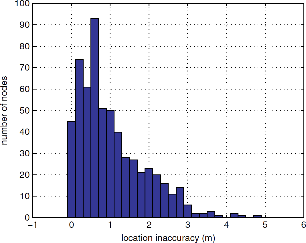
Distribution of nodes' location inaccuracies (N = 600, Γ = 3m).

In addition, we notice that most of the nodes with the location inaccuracy larger than the preset threshold parameter Γ are at the periphery of the circular area. To illustrate this, we use the same simulation as used for Fig. 3, and record all the nodes with a location inaccuracy larger than Γ = 3m (therefore contribute to localization error) as well as plot them as blue stars in Fig. 4. This special characteristic of our partition-based algorithm's localization results is advantageous in the subsequent communication phase, since in the data-collecting networks considered by us, those nodes at the periphery have a low chance to be chosen as relay nodes, and therefore their location inaccuracies are less detrimental with regard to geographic routing.

Figure 4.

Distribution of localization errors (N = 600, Γ = 3m).

Since the measurements are seldom perfect under real wireless sensor network applications, we now simulate the localization performance considering all three possible measurement-related error sources as introduced in the former sections: initial beacon sector error, the TOA measurement noise, and the RSS measurement noise.

We first introduce beacon sector errors into the nodes' initial coarse location information obtained from the BS's broadcasts. The BS's directional beacon broadcasts equally divide the circular network area into M beacon sectors, each with angular range $(k \cdot \frac{2 π}{M}, (k + 1) \cdot \frac{2 π}{M})$ , where k = 0, 1, …, M − 1. Since beacon broadcasts might spray into the neighboring sectors, and because of the characteristics of wireless communications, the nodes close to the sector borders would have a chance to find the beacon indicating the neighboring sector stronger than the beacon indicating its own sector, and mistakenly determine its initial beacon sector number. Considering this, it is reasonable to assume that the nodes within angular range $[k \cdot \frac{2 π}{M} + β, (k + 1) \cdot \frac{2 π}{M} - β]$ are free of beacon sector errors, while any node with an actual angle α within the angular range $[k \cdot \frac{2 π}{M} - β, k \cdot \frac{2 π}{M} + β]$ has beacon sector error probability $\frac{β - | r e m (α, \frac{2 π}{M}) |}{β} \cdot P %$ , where P% is the preset maximal beacon sector error probability parameter, and β is a parameter determined by the sectoring device and wireless transmission conditions. In the simulations, we set $β = \frac{π}{8 M}$ , and set P% = 0.5, while all the other parameters are set to the same as used in the simulations for Fig. 2.

The averaged results of the 50 simulations for both the original and the revised localization algorithms are plotted in Fig. 5. Compared with Fig. 2, it is clear that the localization performance decreases after beacon sector errors are introduced. However, this performance decline can be compensated by increasing network density, since the localization error rate still decreases as the number of nodes increases, and is now kept below 5% when N exceeds 550, and the localization inaccuracy also decreases as N increases, and is now kept below 1.42m. In addition, the revised algorithm's improvements over the original algorithm is not obviously affected by the introduction of beacon sector errors.

Figure 5.

Localization performance with beacon sector errors (Γ = 3m).

To study the TOA and RSS measurement noise's effect, we assume the measured distance to the BS r_measured has the following relationship with the actual distance r_actual: r_measured = r_actual + Δ₁ · ε₁, where Δ₁ is a constant depending on the equipments' parameters and is set to 0.2m, and ε₁ ∼ U(−1, 1); and assume the measured distance between neighbors d_measured has the following relationship with the actual distance d_actual: d_measured = d_actual + Δ₂ · ε₂, where ε₂ ∼ N(0, σ²) and Δ₂ is set to 1m. We increase σ from 0.5 to 2 with step size 0.5; for each value that σ takes, we increase N from 300 to 650 with step size 50, and run the simulation 50 times for each value of N. The results are plotted in Fig. 6, and we also plot the simulation result for the original algorithm with σ set to 2 for performance comparison.

Figure 6.

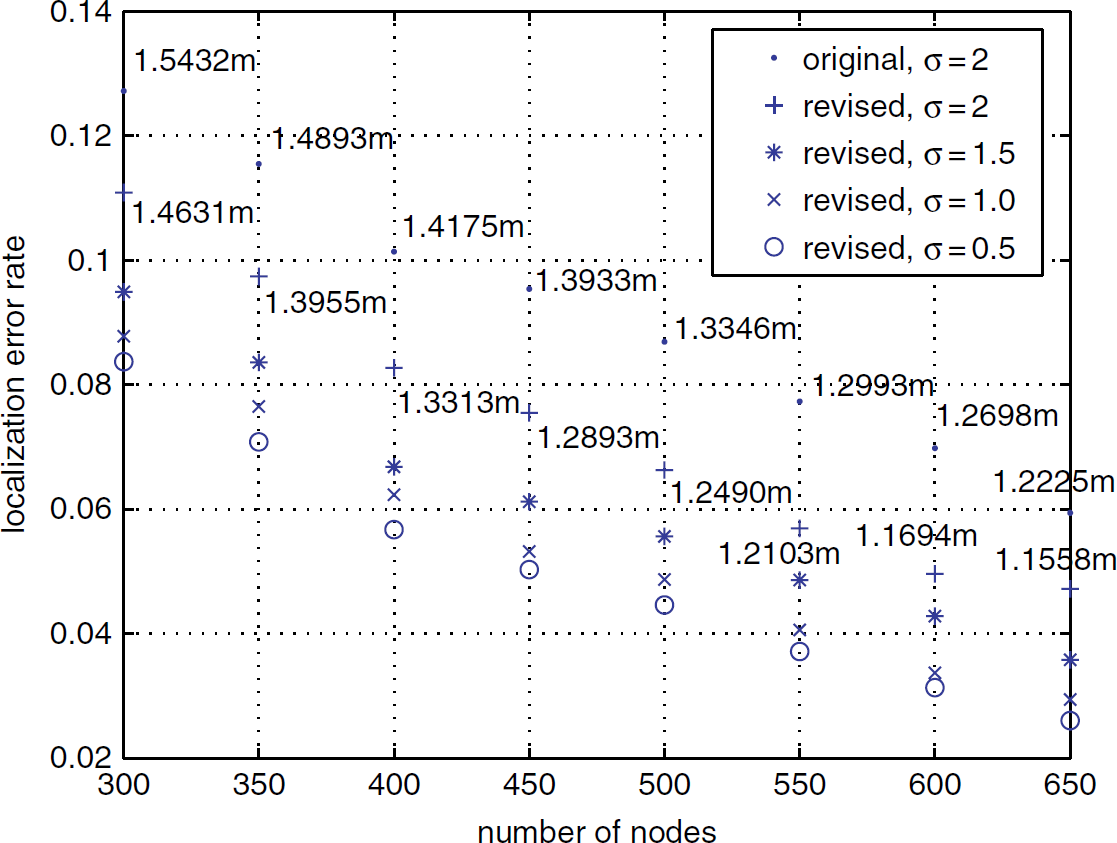
Localization performance with TOA and RSS measurement noises (Γ = 3m).

As expected, the performance of our localization algorithm decreases when there exist TOA and RSS measurement noises. As σ increases, the RSS measurement noise becomes more detrimental, because the estimated distances between neighbors mapped from RSS measurements variate more intensively around the actual distances, which would affect the number of left/right neighbors (n_L/n_R) detected by each node directly, and therefore affect its partition decisions more severely, as we can understand from the flow chart in Fig. 1. However, since the localization performance improves as N increases, our localization algorithm still provides an acceptable performance for high-density networks. In addition, we notice that even for the worst performance case (N = 300, σ = 2) of all simulations, the averaged localization inaccuracy is only 1.4631m; and it decreases monotonically to 1.1558m as N increases to 650, again indicating a pretty good localization performance. And as shown in Fig. 6 for the example case of σ = 2, the revised algorithm's improvements over the original algorithm is not obviously affected by the introduction of TOA and RSS measurement noises.

In Fig. 7, we plot the averaged performance of 50 simulations for both the original and revised algorithms considering all three error sources, with all other simulation settings kept unchanged from Fig. 2. The results can be regarded as the worst case performance of our partition-based localization algorithm since we have set σ to 2. However, acceptable performance can still be achieved provided that the network density is high enough. Thus, our partition-based localization algorithms are better suited for and have larger measurement error tolerance under high-density wireless sensor networks. And as expected, the improvement of the revised algorithm over the original algorithm is still quite obvious.

Figure 7.

Localization performance considering all measurement-related error sources (Γ = 3m, σ = 2).

Since our partition-based localization algorithm provides the information of d_ijmax for each neighboring node pair i and j, which can be used for selecting transmission power in the communication phase, we now use simulations to study our localization algorithm's impacts on communication energy efficiency by studying the distance margins Δd_ij's and average distance margin Δd. The same simulation settings as used for Fig. 7 are applied, thus we are considering the localization performance under worst quality wireless measurements. Since node i and j's wrong partition decisions would probably result in d_ijmax < d_ij (Δd_ij < 0), which would lead to reception failure because not enough transmission power is selected, we refer to this case as “short of distance margin” and pay special attention to it in the simulations. For each value of N, we run the simulation 50 times, and in each simulation, we record those “short of distance margin” neighbor pairs satisfying constraints in equation (3), as well as compute the ratio (distance margin error rate) of the number of these “short of distance margin” neighbor pairs over the total number of neighbor pairs considered by equation (3).

The average of this ratio for these 50 simulations is plotted in Fig. 8 for each value of N. In addition, we mark the averaged $Δ \hat{d}$ of these 50 simulations for each value of N, where $Δ \hat{d}$ differs from the Δd defined in equation (3) only in that those Δd_ij's smaller than 0 are discarded in the summation. The corresponding results of the original algorithm are also indicated for comparison use. Since the “short of distance margin” is caused by neighboring nodes' location inaccuracies, which decrease as the network density increases, the distance margin error rate also decreases as the number of nodes in the network increases as shown in Fig. 8. The revised algorithm has a consistently smaller distance margin error rate than the original algorithm for each value of N, since its corresponding localization error rates and localization inaccuracies are also smaller. Some of the $Δ \hat{d}$ 's for the original algorithm are smaller than the corresponding values for the revised algorithm, one possible reason of which is that a larger portion of big d_ijmax's exceed r_trans and thus are not included in the computation of $Δ \hat{d}$ for the original algorithm, which results in a smaller partial averaging.

Figure 8.

Distance margin error rate considering all measurement-related error sources (Γ = 3m, σ = 2).

Fig 9 shows the distribution of the distance margins of the neighbor pairs satisfying equation (3)'s constraints in one simulation. It is obvious that most of the distance margins are around the average distance margin ( $Δ d = 1.6701 m, Δ \hat{d} = 1.9020 m$ in this simulation), and therefore the average distance margin Δd (adjusted average distance margin $Δ \hat{d}$ ) is a reasonable metric to evaluate our partition-based localization algorithm's impacts on communication energy efficiency.

Figure 9.

Distribution of neighbor pairs' distance margins (N = 650, Γ = 3m, σ = 2).

5. Geographic Routing Algorithm

We consider a data-collecting wireless sensor network with most of its traffic from sensor nodes uniformly distributed in a circular network area to the sink node at the center of the circular area, and apply the following energy model:

Energy consumption for sensing and generating a data packet is: e_s = α₁; energy consumption for receiving a data packet is: e_r = α₂; energy consumed by node i to transmit a data packet to neighboring node j with distance d_ij is: e_t(i, j) = α₃ + α₄ · d_ijⁿ.

With the above energy model, we can study the choice between direct and relay transmission.

Consider two nodes A and B within each other's communication range and with distance relationship: |AB| = d. To deliver a data packet directly from A to B, the total energy consumed by this two-node system is: e₁ = e_AB = α₃ + α₄ · dⁿ + α₂. While if we have a third node C between nodes A and B with |AC| = x, |CB| = d − x, and act as a relay node, the total energy consumed by this three-node system is:

e_{2} = e_{AC} + e_{CB} = α_{3} + α_{4} \cdot x^{n} + α_{2} + α_{3} + α_{4} \cdot (d - x)^{n} + α_{2}

To make e₁ > e₂, we need: g(x) = α₄ · (xⁿ + (d − x)ⁿ − dⁿ) + α₃ + α₂ < 0, where g'(x) = α₄ · n · (xⁿ⁻¹ − (d − x)ⁿ⁻¹) achieves 0 when x = d/2.

Since the value of n is between 2 and 4, g'(x) < 0 if x < d/2, and g'(x) > 0 if x > d/2, therefore function g(x) attains global minimum at x = d/2.

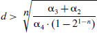
Let g(d/2) < 0, we can deduce the necessary condition for preferring using a middle node C as relay node:

d > \sqrt[n]{\frac{α_{3} + α_{2}}{α_{4} \cdot (1 - 2^{1 - n})}}

Since our partition-based localization algorithm has better performance for high-density wireless sensor networks, we focus on these types of networks from now on. Thus it is reasonable to assume that we can find a large number of candidate relay nodes between each pair of source and destination. Suppose the distance between source A and destination B satisfies $| AB | = d > \sqrt[n]{\frac{α_{3} + α_{2}}{α_{4} \cdot (1 - 2^{1 - n})}}$ , thus the relay transmission is preferred over direct transmission, and we now deduce the most energy efficient relay nodes arrangement.

Suppose we use k nodes in a line with A, B as relay nodes, namely C₁, C₂, C₃, …, C_k, with distance relationship |AC₁|=x₁, |C₁C₂|=x₂, |C₂C₃|=x₃, …, |C_kB|=x_k+1, and d = x₁ + x₂ + x₃ + … + x_k + x_k+1. Using a similar process as above, we can deduce that minimum energy consumption is achieved when we let x₁ = x₂ = x₃ = … = x_k = x_k+1 = d/(k + 1), and the energy consumed for one packet is: $g (k) = (α_{4} \cdot (\frac{d}{k + 1})^{n} + α_{3} + α_{2}) (k + 1)$ , where g'(k) = α₄ · dⁿ · (1 - n) · (k + 1)⁻ⁿ + α₂ + α₃ achieves 0 at $k_{optimal} = d \cdot \sqrt[n]{\frac{α_{4} \cdot (n + 1)}{α_{3} + α_{2}}} - 1$ .

Since n is between 2 and 4, we have g'(k) < 0 when k < k_optimal, and g'(k) > 0 when k > k_optimal, therefore, function g(k) attains a global minimum at k = k_optimal.

Thus, we arrive at the following Minimal Energy Consumption Routine for selecting relay nodes:

Given a source node and a destination node with distance d, direct transmission is always better if $d \leq \sqrt[n]{\frac{α_{3} + α_{2}}{α_{4} \cdot (1 - 2^{1 - n})}}$ , while if $d > \sqrt[n]{\frac{α_{3} + α_{2}}{α_{4} \cdot (1 - 2^{1 - n})}}$ , energy consumed for communication is minimized when we use k_opt = ⌊k_optimal⌋ or ⌈k_optimal⌉ relay nodes, all of which are equally distributed in a line between source and destination, where $k_{optimal} = d \cdot \sqrt[n]{\frac{α_{4} \cdot (n - 1)}{α_{3} + α_{2}}} - 1$ .

Now suppose node i has data to send to the BS, and node j is in node i's neighbor list with r_j < r_i. Energy consumed to send a data packet directly from i to the BS is

e_{i \to BS} = {\begin{cases} α_{3} + α_{4} \cdot r_{i max}^{n} & : r_{i max} \leq r_{trans} \\ + \infty & : r_{i max} > r_{trans} \end{cases}

(4)

Where we take r_imax = r_i + Δ₁ as node i's distance to the BS to insure successful reception with the existence of TOA measurement noise.

Since we are proposing a geographic routing algorithm whose operation is based on the results of our partition-based localization algorithm, a node i can use d_ijmax stored in its neighbor list instead of d_ij estimated from RSS while making transmission power selections to increase successful reception rate at its neighbor j. And as we are studying high-density sensor networks, it is reasonable to assume that relay node j could always arrange the subsequent relay nodes according to the minimal energy consumption routine. Thus, the energy consumption of the network for relay transmission one data packet starting from node i using node j as the first relay node is

\begin{aligned} e_{relay} = & e_{i \to j} + e_{j \to BS} \\ = & (α_{3} + α_{4} \cdot {d_{i j max}}^{n}) \\ + (α_{2} + α_{3} + α_{4} \cdot {(\frac{r_{j max}}{{\tilde{k}}_{opt} + 1})}^{n}) ({\tilde{k}}_{opt} + 1) \\ \approx & (α_{3} + α_{4} \cdot {d_{i j max}}^{n}) \\ + (α_{2} + α_{3} + α_{4} \cdot {(\frac{r_{j max}}{{\tilde{k}}_{optimal} + 1})}^{n}) ({\tilde{k}}_{optimal} + 1) \\ = & (α_{3} + α_{4} \cdot {d_{i j max}}^{n}) \\ + (α_{2} + α_{3}) \cdot \frac{n}{n - 1} \cdot r_{j max} \cdot β \end{aligned}

(5)

Where $β = \sqrt[n]{\frac{α_{4} \cdot (n - 1)}{α 3 + α 2}}, {\tilde{k}}_{optimal} = r_{j max} \cdot β - 1$ , and ${\tilde{k}}_{opt} = ⌊ {\tilde{k}}_{optimal} ⌋ or ⌈ {\tilde{k}}_{optimal} ⌉$ .

To avoid overly utilizing pivotal nodes so as to keep the network responsive to events arising everywhere and thus have a longer lifetime, we need to take into consideration candidate relay node's current energy levels while making routing decisions. Thus we can introduce energy-awareness into our geographic routing algorithm by revising formula (5) into some weighed relay energy consumption formula utilizing the energy level indicator l_j's stored in node i's neighbor list as suggested in [18]. However, this is not the focus of this paper and the following performance evaluations, and more exploration is to be done as our future work.

Now we can summarize our geographic routing algorithm as follows:

If a node i has data to send, it traverses its neighbor list and compares the energy consumption of relay transmission through each neighbor j (computed using formula (5)) with the energy consumption of direct transmission (computed from formula (4)). If the energy consumption of direct transmission is the smallest, node i transmits directly to the sink; otherwise, the neighbor j with the smallest relay energy consumption is chosen to be the next relay node.

It is obvious that our geographic routing algorithm is loop-free, and it is indeed localized since each node makes routing decisions in consideration of minimizing the whole network's energy consumption with only local information (its own neighbor list).

6. Performance Evaluations of the Combined Localization and Geographic Routing Algorithm

So as to prove the effectiveness of our combined design of the localization and routing algorithm, we now show that our geographic routing algorithm does manage to avoid most of the location estimation errors' impacts. Thus, we will compare the performance of our combined partition-based localization and geographic routing algorithm, with that of our geographic routing algorithm utilizing perfect location information, for which the performance metric of the packet drop rate and average path inefficiency are introduced.

We define the packet drop rate as the ratio of the number of data packets dropped during the transmission to the sink over the total number of data packets generated for the sink. According to our geographic routing algorithm, packet drops might be caused by not enough transmission power being selected, or no candidate relay node with enough energy being present. To better focus on the location estimation errors' impacts, we assume all the nodes have enough energy during this evaluation process, and calculate the packet drop rate for the first 500 randomly generated data packets. Thus, in a sensor network with high node density, packet drops using the results of our partition-based localization algorithm, are caused by “short of distance margin,” e.g., due to the wrong sub-sector decisions by either node i or node j or both of them during the localization process, the transmission power is selected using d_ijmax < d_ij at node i, and therefore not enough to ensure successful reception at node j. To focus on the impact of “short of distance margin” cases, we assume the packet drop rate under perfect location information to be zero, thus ignoring the wireless communication disturbance's effects. In other words, we study the relative packet drop rate of our combined algorithm with regard to that of our routing algorithm utilizing perfect location information.

We define the path inefficiency of a data packet originating at node i as the ratio of the length of the path selected by our routing algorithm over the actual distance r_i from node i to the BS and then minus one. The path inefficiency of our routing algorithm utilizing perfect location information might be greater than zero, since nodes' distribution and energy status do not always allow strait-line transmission path; the average path inefficiency of our combined localization and routing algorithm would be greater than zero for the same reason, and in addition because d_ijmax and r_jmax are used instead of d_ij and r_j while making routing decisions. To better focus on the location inaccuracies' impacts, we again assume all the nodes have enough energy during this evaluation process, and define the average path inefficiency as the averaged inefficiency values of the first 400 randomly generated data packets that are successfully delivered to the sink.

The simulation settings are as follows: assume a circular data-collecting sensor network with radius R = 50m and the sink node at the center, there are N nodes of 2-D uniform distribution in the network area, each with the same adjustable transmission power and maximal transmission range r_trans = 15m. The parameters used in the energy model are set according to [19]: α₁ = 50nJ, α₂ = 135nJ, α₃ = 45nJ, α₄ = 1nJ/m² (n = 2).

Since our partition-based localization algorithm has a higher performance with higher node density under severe measurement noises, we assume the existence of all the three introduced measurement error sources in the worst case, and thus set N = 650. We run the simulation 20 times: in each simulation, firstly N nodes are randomly distributed in the circular area, and the partition-based localization algorithm is carried out at each node. Then the nodes collaborate according to the geographic routing algorithm introduced before to report randomly arising events, and the relative packet drop rate for the first 500 data packets for the case of routing based on partition-based localization results with regard to that of routing based on perfect location information is calculated and plotted in Fig. 10; while the average path inefficiency for the first 400 successfully delivered data packets is calculated and plotted for both of these two cases as well in Fig. 11.

Figure 10.

Packet drop rate of the geographic routing algorithm considering all measurement-related error sources (N = 650, Γ = 3m, σ = 2).

Simulations for Fig. 10 show that, under severe measurement noises (σ = 2) and with beacon sector errors, the averaged distance margin error rate of these 20 simulations is 9.12% with standard deviation 0.0116, while the averaged packet drop rate is 6.04% with standard deviation 0.0139. Thus, a large portion of the distance margin errors do not result in delivery failure, and therefore our geographic routing algorithm does effectively avoid location estimation errors' impacts as we expected.

As we can see from Fig. 11, the average path inefficiency of our geographic routing algorithm with perfect location information is above 0 for all simulations, and has averaged value 0.0288 and standard deviation 0.0105 for these 20 simulations. This is because the nodes' distribution does not always support straight-line paths while the network energy consumption is to be minimized. The average path inefficiency of our combined localization and routing algorithm has a larger averaged value of 0.0784 and standard deviation 0.0107 for these 20 simulations, since the location information available after the partition-based localization process is fan-shaped areas instead of exact points, and under the assumption of severe measurement noises and beacon sector errors, d_ijmax's and r_jmax's would be much larger than d_ij's and r_j's, which leads to a relatively higher inefficiency value when applied in route selections and path length calculations. However, since perfect location information has to come from GPS equipments which are not appropriate for high-density sensor networks considering both cost and energy-consumption constraints, our simple localized partition-based localization algorithm is still preferred when our geographic routing algorithm is to be applied, only at a slight performance degradation.

Figure 11.

Average path inefficiency of the geographic routing algorithm considering all measurement-related error sources (N = 650, Γ = 3m, σ = 2).

7. Conclusions

In this paper, we proposed a partition-based localization algorithm for rapidly-deployed wireless sensor networks, and a routing algorithm that effectively uses its coarse-grained localization results to minimize energy consumption. During the localization process, each node broadcasts messages of a preset format and collects one-hop neighbors' messages to keep its neighbor list up to date. The BS originally divides the circular network area into M beacon sectors, and then each node keeps partitioning its current sector and locating itself in a smaller sub-sector with the help of its neighbor list till the localization termination condition is satisfied. The routing algorithm uses a minimal energy consumption routine to select transmission mode (direct/relay) as well as relay nodes, and only takes as input the neighbor list generated from the localization process besides the current node's own localization result. Thus, both algorithms are localized and scale well with the size of the network. Simulation results confirmed that our localization algorithm's performance improves with node density, and is robust against the measurement noise; while our combined localization and routing algorithm achieves high energy efficiency at low cost and has comparable performance with the same routing algorithm utilizing perfect location information even under severe measurement noises, thus proofs the effectiveness of our combined design.

References

Lukachan

and Labrador

M. A.

, “SELAR: Scalable energy-efficient location aided routing protocol for wireless sensor networks”, in Proceedings LCN'04, November 16–18, 2004.

Doherty

Pister

, and Ghaoui

, “Convex position estimation in wireless sensor networks”, in Proceedings IEEE InfoCom, April 2001, Anchorage, AK.

Bulusu

Heidemann

, and Estrin

, “GPS-less low cost outdoor localization for very small devices,” IEEE Personal Communications Magazine, October 2000, vol. 7, no. 5, pp. 28–34.

Huang

Lum

Stankovic

, and Adelzaher

, “Range-free localization schemes for large scale sensor networks”, in Proceedings ACM MobiCom, September 2003, San Diego, CA.

Niculescu

and Nath

, “Ad Hoc Positioning Systems”, in Proceedings GlobeCom, November 2001.

Lei

and Ning

, “A beacon-less location discovery scheme for Wireless sensor networks,” InfoCom'2005, Miami, Florida.

Y. B.

and Vaidya

N. H.

, “Location-aided routing(LAR) in mobile ad hoc networks”, in Proceedings MobiCom'98, October 1998, Dallas, TX, pp. 66–75.

Basagni

Chlamtac

and Syrotiuk

, “Geographic messaging in wireless ad hoc networks”, in Proceedings the 49th IEEE Int. Vehicular Technology Conference, 1999, Houston, TX, vol. 3, pp. 1957–1961.

Basagni

Chlamtac

Syrotiuk

V. R.

and Woodward

B. A.

, “A distance routing effect algorithm for mobility (DREAM)”, in Proceedings MobiCoM'98, October 1998, Dallas, TX, pp. 76–84.

10.

Karp

and Kung

H. T.

, : “GPSR Greedy perimeter stateless routing for wireless networks,” in Proceedings the 6th Annual International Conference on Mobile Computing and Networking, Aug. 2000, Boston, Massachusetts, pp. 243–254.

11.

Kuhn

Wattenhofer

and Zollinger

, “Worst-case optimal and average-case efficient geometric ad-hoc routing”, in Proceedings ACM MobiHoc, June 2003, Annapolis, MD.

12.

Jain

Puri

, and Sengupta

, “Geographical routing using partial information for wireless ad hoc networks,” IEEE Personal Communications, February 2001, 8(1):48(r)C57.

13.

Melodia

Pomppili

, and Akyildiz

I. F.

, “Optimal local topology knowledge for energy efficient geographical routing in sensor networks”, in Proceedings IEEE InfoCom, March 2004, Hong Kong, China.

14.

Pei

Gerla

, and Chen

T. W.

, “Fisheye state routing: A routing scheme for ad hoc wireless networks”, in Proceedings IEEE ICC, June 2000, New Orleans, LA.

15.

Witt

and Turau

, “The impact of location errors on geographic routing in sensor networks,” in Proceedings ICWMC'06, July 29(r)C31, 2006, Bucharest, Romania.

16.

Hui

and Wicker

Stephen B.

, “Anchor-free localization in rapidly-deployed wireless sensor networks,” in Proceedings of 2006 IEEE International Conference on Mobile Ad Hoc and Sensor Systems (MASS), pp. 627–632.

17.

Subramanian

and Shakkottai

, “Geographic routing with limited information in sensor networks”, in Proceedings IPSN 2005.

18.

Hui

and Wicker

Stephen B.

, “Co-designed anchor-free localization and location-based routing algorithm for rapidly-deployed wireless sensor networks,” submitted to Information Fusion.

19.

Heinzelman

, “Application-specific protocol architectures for wireless networks”, Ph.D dissertation, Massachusetts Institute of Technology, 2000.