Sage Journals: Discover world-class research

Abstract

Real-time tracking of moving targets using wireless sensor networks has been a challenging problem because of the high velocity of the targets and the limited resources of the sensors. CPA (closest point of approach) algorithms are appropriate for tracking fast-moving targets since the tracking error is roughly inversely proportional to the square root of the target velocity. However, this approach requires a specific node configuration with reference to the target trajectory which may not always be possible in randomly deployed sensor networks. Moreover, our mathematical analysis of the original CPA algorithm shows that it suffers from huge localization errors due to inaccuracies in sensor location and measured CPA times. To address these issues, we propose an enhanced CPA (ECPA) algorithm which requires only five sensors around the target to achieve the reliability and efficiency we want for computing the bearing of the target trajectory, the relative position between the sensors and the trajectory, and the velocity of the target. To validate the ECPA algorithm, we designed and implemented this algorithm over an actual data-centric acoustic sensor network as well as simulating it in an NS-2 simulator. The results of our field experiments and simulations show that we can achieve our goals of detecting the target and predicting its location, velocity and direction of travel with reasonable accuracy.

Keywords

Real-Time Target Tracking Closest Point of Approach Algorithm Collaborative Mixed Wireless Sensor Networks Acoustic Sensor Networks High-Speed Target Tracking Distributed Algorithms

1. Introduction

Wireless sensor networks are composed of relatively inexpensive sensors capable of collecting, processing, storing, and transmitting information among networks. An interesting application of wireless sensor networks (WSN) is target localization and tracking in a hostile environment, where physical access is accompanied by some form of danger (e.g., the battlefield).

Due to the high velocity of targets and limited resource of sensors, localization and tracking of moving vehicles is a challenging problem in WSN. First, the localization algorithm must perform well (localization error must be very low, e.g., 3 m), regardless of the high speed of the mobile target, i.e., higher velocity must not cause higher localization errors. Second, the entire system must be energy efficient. Since network communication consumes significantly more power than the local computation, the size and number of messages exchanged among sensors should be minimized. Third, due to the limited capacity of each sensor, tracking a mobile target requires multiple nodes to collaboratively share information between each other. Fourth, target tracking has much higher requirement than target localization since velocity and direction of movement are also required for tracking purpose. Fifth, the tracking algorithm must meet the real-time deadlines of the target tracking application. It must be as fast as (or faster than) the velocity of the vehicle.

To meet these design requirements, the CPA (closest point of approach) algorithm [1, 2] is one of the best candidates. The CPA algorithm is well suited for tracking targets at high speeds. In fact, higher speeds result in lower localization error. In addition, the only information exchanged between sensors is the measured CPA time, so the size of the exchanged message is very small. Furthermore, the algorithm not only calculates the target position but also the velocity and moving direction of the target. Therefore, we have adopted the CPA based algorithm for our target tracking system.

The original CPA algorithm, however, cannot be directly applied to wireless sensor networks because specific deployment configurations of sensors are required [1, 2]. For instance, in [1] the target trajectory must intersect the convex hull composed of sensors without evenly splitting the sensor field, while in [2], the target trajectory must be located outside the convex hull of sensors. In a realistic system, the target will trigger a set of sensors that may not satisfy the configuration requirements. Moreover, due to the measurement errors in sensors location and CPA times, there will be huge errors in locating the target trajectory. In most cases, the original CPA algorithm may completely fail to localize the target because of the large errors in input parameters. Therefore, neither of the CPA algorithms [1, 2] may be directly used.

To solve these problems, we developed an enhanced the CPA (ECPA) algorithm. It first determines the network configuration based on CPA times at the sensors, and then selects four nodes which satisfy the node deployment requirement of the original CPA algorithm. By running the original CPA algorithm, four possible trajectory directions can be obtained, and the one which is closest to the estimated slope of the target trajectory will be considered the correct one. Finally, the trajectory location is recomputed based on the newly calculated direction information. Our mathematical analysis of the ECPA algorithm shows that it results in much smaller errors in localizing the target trajectory than the original CPA algorithms. Simulations and field experiments verify that the ECPA algorithm causes very small localization errors.

There are four main contributions in this paper. First, we have developed the ECPA algorithm that effectively computes the target location, velocity, and direction in wireless sensor networks composed of low-powered, inexpensive nodes. Second, we performed a mathematical analysis of both ECPA and CPA algorithms, and have shown that the ECPA algorithm performs well in WSN and generates much smaller errors in locating target trajectory. Third, we have implemented the ECPA algorithm in both simulations and field experiments. The results also confirm that the ECPA algorithm is more efficient for the real-time target tracking. Fourth, we designed and implemented a sensor networking system that integrates and interoperates the ECPA algorithm for accurately computing target location, velocity, and direction with control software for controlling video sensor nodes that capture image or video of the target at its predicted location.

2. Related Work

There are many research efforts on target detection and tracking in wireless sensor networks that describe several aspects of collaborative signal processing [3–6], target tracking with camera sensors [7], and real-time application for field biologists to discover the presence of individuals [8]. Recently, a set of approaches [9–12] were proposed to solve the target localization and tracking problem with proximity binary sensors which report only one bit information to indicate if a target appears. Though the information transmitted in networks was reduced, the localization error was increased. As proven in [10], the achievable spatial resolution in localizing a target trajectory is of the order of 1/(ρR), where R is the sensing radius and ρ is the sensor density per unit area. Suppose there are 25 sensors, with a sensing radius of 20 m, deployed in a 100 × 100 m² area, then the lower bound of the localization error will be 20 m. Therefore, it is only suitable for very dense sensor networks.

Collaborative signal processing methods, such as the Extended Kalman Filter (EKF), were first used for target tracking in [6, 13], in which fused tracks are processed to predict their future trajectories and this is similar to predicting the state and error covariance at the next time step given the current information using the Kalman filter algorithm. The predicted future track determines the regions likely to detect the entity in the future. These algorithms can effectively localize and track moving targets, but involves too much computation overhead on sensors. Thus, they are inefficient for wireless sensor networks.

In the area of acoustic sensor networks, there are many solutions for target localization and tracking which can be divided into three basic categories: differential signal amplitude (DSA) [14, 15], direction of arrival (DOA) [8, 16] and time difference of arrival (TDOA) [17, 18]. DSA is used by [14, 15] with the assumption that the acoustic energy decays as the inverse of the distance square under certain conditions. However, the main problem with the differential signal amplitude method is that calculating the distance based on the received signal strength is very error-prone. Because the accuracy of the RSSI (received signal strength indication) range measurements is highly sensitive to multi-path fading, non-line-of-sight scenarios, and other sources of interference, this method may result in large errors. These errors can propagate through all subsequent triangulation computations, leading to large localization errors. Other methods [8, 16] make use of the DOA (of the acoustic signal generated by the target) information from different spatially separated sensors, to estimate the target location. However, there are various factors that affect the accuracy of the DOA estimates: accuracy of the hardware used to capture the array signals, sampling frequency, number of microphones used, reverberation and noise present in the signals. Moreover, DOA estimation requires a microphone sub-array on each sensor, which will increase not only the cost of deployment but also the signal processing overhead on sensors. TDOA methods [17, 18] make use of the relative time differences among sensors. To obtain the relative time difference, each sensor needs to first get the dominant frequency of the acoustic spectrum, and then broadcast this information [17, 18]. This may involve collaborative signal processing, such as FFT, which will increase the computational overhead. On the other hand, the audio data exchanged among sensors requires more network bandwidth, a very precious resource in wireless sensor networks.

We chose the CPA target tracking algorithm [1] to estimate the target position, velocity, and moving direction. Intuitively, the CPA time is the instance when the target was at the closest point to a sensor node. Although it belongs to the TDOA category, the CPA algorithm only requires the CPA time to be stored and exchanged among sensors instead of the audio data used in [17, 18]. Since the CPA time could be stored in four bytes (two for the integer and the others for the decimal), the message exchange overhead is low. As previously described, the original CPA algorithm [1, 2] cannot be directly used for wireless sensor networks because of the specific sensor deployment requirements. The ECPA algorithm, however, does not have such network configuration requirements and can also reduce the localization error caused by the uncertainties in the position and the CPA time determination. Therefore, to the best of our knowledge, we are the first to apply an enhanced CPA algorithm in a practical wireless sensor network, composed of acoustic sensors, to localize and track moving targets.

3. Target Localization Algorithm

3.1. Original CPA Algorithm

The CPA (closest point of approach) algorithm was originally designed for localizing low-flying aircraft by means of acoustic sensors [1]. The problem is first formulated in the three-dimensional case and then specialized to the case when the target and sensors are all in one plane. A similar approach was proposed in [2], which requires three non-collinear sensors deployed on the same side of the target trajectory. The trajectory direction can be calculated by solving a single linear equation with the sine and cosine of the angle formed by the target trajectory and a reference axis. Then, the source speed can be computed by a single linear equation. One assumption of the CPA algorithm is that the target moves with a constant velocity (i.e., linear path) while passing through the set of nodes (either three [2] or four [1] sensors). This assumption is necessary because of the limited detection range of low-powered sensor nodes and the high speed of the target. For example, suppose there are 25 sensors uniformly distributed in a 100 × 100 m² area, the sensing range is 20 m, and the target speed is 30 miles/hour. Then within 5 sec, the target will trigger on the average six sensors around the trajectory, which meets the requirement of the CPA algorithm. We argue that within a short time interval, e.g., 5 sec, the target speed can be considered constant with very small variation.

To make the original CPA algorithm amenable to programming, we reformulate the equations as follows. As shown in Fig. 1, v and r denote the target velocity and the distance of the closest point of approach to the origin of the coordinate system, respectively. Then the target path is given by:

p (t) = r + v (t - r), τ^{T} v = 0

(1)

where ^T denotes the transpose of a certain vector and τ the instance at which the target moves through r. Let r_k denote the position vector of node k and t_k the measured CPA time. We define the CPA time as the time when the target reaches the closest point of approach, and the measured CPA time as the instance at which the received signal amplitude reaches the highest at the sensor. Therefore, the difference between those two will be the time of sound propagation from the closest point of approach to the sensor. Then we can define t_k as:

| p (t^{'}) - r_{k} | \to min, | p (t^{'}) - r_{k} | = c (t_{k} - t^{'})

(2)

where |·| is the Euclidian norm and c the velocity of sound. Using Eq. (1) to solve the minimal t and inserting the result into the Eq. (2) yields:

| r - r_{k} + (v^{T} r_{k}) v / υ^{2} | = c (t_{k} - τ - v^{T} r_{k} / υ^{2})

(3)

where υv = |v|. The left side of Eq. (3) can be rewritten as:

| r - \frac{r_{k} \cdot r^{T} \cdot r}{r^{T} \cdot r} + \frac{(v^{T} r_{k}) v \cdot r \cdot r^{- 1}}{v^{2}} |

(4)

Figure 1.

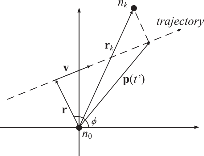
Illustration of CPA localization and tracking algorithm.

In the two-dimensional case, r and v are orthogonal, so Eq. (4) can be simplified as:

| r - (r_{k} r^{T}) r / | r |^{2} | = | r | \cdot | 1 - r_{k} r^{T} / r^{2} |

(5)

Thus, Eq. (3) becomes:

r | r_{k}^{T} r / r^{2} - 1 | = c (t_{k} - τ - v^{T} r_{k} / v^{2})

(6)

For convenience, we place the origin of the coordinate system onto one of the sensors, e.g., n₀ (r₀ = 0). So t₀ is the measured CPA at node n₀. Subtracting r = c(t₀ - τ) from Eq. (6) yields:

r (| r_{k}^{T} r / r^{2} - 1 | - 1) + (c / v^{2}) r_{k}^{T} v = c (t_{k} - t_{0}) = d_{k}

(7)

Let r_k = (x_k, y_k)^T and let ϕ and M be defined by:

r = r (\cos ϕ, \sin ϕ)^{T}, (c / v^{2}) v = M^{- 1} (- \sin ϕ, \cos ϕ)^{T}

(8)

Then, the Mach number M is positive or negative depending on whether the target crosses the CPA from right to left or left to right, as observed from the origin point. If the target trajectory intersects the line r₀r_k, which also means $r_{k}^{T} r / r^{2} - 1 \geq 0$ , then Eq. (7) becomes:

x_{k} cos ϕ + y_{k} sin ϕ + (- x_{k} sin ϕ + y_{k} cos ϕ) / M - 2 r = d_{k}

(9)

Otherwise, if the trajectory does not intersect line $r_{0} r_{k} (i.e., r_{k}^{T} r / r^{2} - 1 < 0)$ , we have:

- x_{k} cos ϕ + y_{k} sin ϕ + (- x_{k} sin ϕ + y_{k} cos ϕ) / M = d_{k}

(10)

In both Eqs. (9) and (10), there are three unknown variables ϕ, M and r. As M = v/c, the three target motion parameters ϕ, v and r can be calculated if we have three equations. Therefore, except for the origin node, three more sensors are needed, i.e., four sensors should be enough to solve the problem and compute the target motion parameters. However, the method in [1] will fail if the trajectory generates an even decomposition of the sensor field, in which two sensors are on one side of the trajectory and others are on the other side, because the resulting equation of M will be of fourth degree and must be solved numerically.

To solve the localization problem, the trajectory must unevenly divide the four sensors into two groups: three on one side and one on the other side. To ensure that this situation occurs, we need to collect information from five sensors. The next section will discuss this process in detail. Now suppose the origin of the coordinate system is at n₀ which is the lone node, then we have the following equation:

x_{k} cos ϕ + y_{k} sin ϕ + (- x_{k} sin ϕ + y_{k} cos ϕ) / M - 2 r = d_{k}

(11)

where k = 1, 2, 3. By subtracting any two of the above equations, we will obtain two formulas. For example:

(x_{1} - x_{3}) cos ϕ + (y_{1} - y_{3}) sin ϕ + [(x_{3} - x_{1}) sin ϕ + (y_{1} - y_{3}) cos ϕ)] / M = d_{1} - d_{3}

(12)

(x_{1} - x_{3}) cos ϕ + (y_{2} - y_{3}) sin ϕ + [(x_{3} - x_{2}) sin ϕ + (y_{2} - y_{3}) cos ϕ)] / M = d_{2} - d_{3}

(13)

Combining these two with Eq. (11) when k = 3, yields:

ξ_{k} \cos ϕ + η_{k} \sin ϕ + (- ξ_{k} \sin ϕ + η_{k} \cos ϕ) / M = δ_{k}

(14)

x_{3} \cos ϕ + y_{3} \sin ϕ + (- x_{3} \sin ϕ + y_{3} \cos ϕ) / M - 2 r = d_{3}

(15)

where k = 1, 2, ξ_k = (x_k - x₃), η_k = (y_k− y₃) and δ_k = (d_k - d₃). By multiplying Eq. (14), relative to specific k value (k = 1, 2), with ξ_3−k and subtracting them, we obtain:

δ_{1} ξ_{2} - δ_{2} ξ_{1} = (- η_{1} ξ_{2} + η_{2} ξ_{1}) \sin ϕ + (η_{1} ξ_{2} - η_{2} ξ_{1}) \cos ϕ / M

(16)

Multiplying Eq. (14), relative to specific k value (k = 1, 2), with η_3−k and subtracting them again gives:

δ_{1} η_{2} - δ_{2} η_{1} = (- η_{2} ξ_{1} + η_{1} ξ_{2}) \cos ϕ + (η_{2} ξ_{1} - η_{1} ξ_{2}) \sin ϕ / M

(17)

Adding the square value of Eq. (16) and (17), yields:

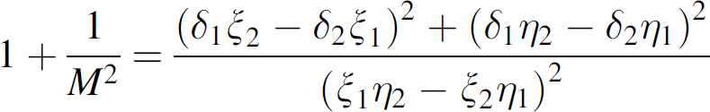
1 + \frac{1}{M^{2}} = \frac{(δ_{1} ξ_{2} - δ_{2} ξ_{1})^{2} + (δ_{1} η_{2} - δ_{2} η_{1})^{2}}{(ξ_{1} η_{2} - ξ_{2} η_{1}) 2}

(18)

Now since all the variables δ₁, ξ₁, η₁, δ₂, ξ₂, η₂ are known, then two possible M can be computed. As we mentioned above, the Mach number M is positive or negative depending on whether the target crosses the origin from right to left, or vice versa. Therefore, by checking the position of nodes with the earliest and latest measured CPA times, the target moving direction can be determined easily.

Then Eq. (14) can be rewriten as:

(- ξ_{k} + \frac{η_{k}}{M}) \cos ϕ + (- η_{k} - \frac{ξ_{k}}{M}) \sin ϕ - δ_{k} = 0

(19)

Given the computed M and $cos ϕ = \pm \sqrt{1 - {sin}^{2} ϕ}$ , four possible value of ϕ will be generated by solving the previous equation. According to the original CPA algorithm, by inserting M and each ϕ into Eq. (11), r can be obtained. If r < 0 or the computed trajectory does not match the assumed sensor field decomposition, the value of ϕ will be rejected; otherwise, it is accepted as correct.

3.2. Impact of Sensors Location Error

As discussed in [1], assuming the measured CPA times are unbiased and normally distributed, the target localization errors (including three motion parameters, ϕ, v, and r) of the original CPA algorithm can be calculated through the Fisher information matrix. Although the errors caused by measuring CPA times are very small, that analysis ignored the impact of sensors location error which may cause the original CPA algorithm to fail in most cases. In this section, we will discuss the influence of sensors location error on the computation of distance r and angle ϕ. Accordingly, we describe the reason why the original CPA algorithm cannot be directly applied to sensor networks and how to modify it to correct the problem.

3.2.1. Sensitivity of Distance Computation

In the original CPA algorithm, the error in the computation of distance r is very large because of the errors in the sensor location and the measured CPA time.

There are many methods to obtain sensor locations although these are outside the scope of this paper. Instead, we simply assume sensors know their positions through GPS (Global Positioning System). However, the localization accuracy of the GPS system could be affected by many factors (e.g., the ionosphere error, satellite clock error, orbit error, troposphere error, and multi-path error). The localization error in GPS with a C/A code receiver and either standard correlator or narrow correlator ranges from 0.1 to 3 meters [19]. For other methods, e.g., triangulation, the error may be even larger.

We now describe how sensitive the original CPA algorithm is to errors in sensor locations and measured CPA times. Suppose the angle of vector r_k is β, then Eq. (11) becomes:

r_{k} \cdot \cos β \cdot \cos ϕ + r_{k} \cdot \sin β \cdot \sin ϕ + (r_{k} \cdot \sin β \cdot \cos ϕ - r_{k} \cdot \cos β \cdot \sin ϕ) / M - 2 r = d_{k}

(20)

It can be rewritten as:

r_{k} \cdot \cos (β - ϕ) + r_{k} \cdot \sin (β - ϕ) / M - 2 r = d_{k}

(21)

Small changes in r_k and (t_k - t₀) yield a small change in r as follows:

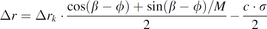
Δ r = Δ_{r_{k}} \cdot \frac{\cos (β - ϕ) + \sin (β - ϕ) / M}{2} - \frac{c \cdot σ}{2}

(22)

where σ = Δ(t_k - t₀). Assume t₀ is accurately measured, then σ becomes Δt_k that denotes the bias in the CPA estimates at node n_k. Suppose Δr_k = 2 m, then the error in computed r is shown in Fig. 2, where the x-axis is the error in measured CPA times and the y-axis is the value of (β - ϕ). Since node n₀ and n_k are on different sides of the trajectory, the angle between r and r_k will range from −90° to 90°.

Figure 2.

Error in the computed r in the original CPA algorithm.

By investigating Eq. (22) further, we find that the left and the right side of the equation indicates the error in computed r caused uncertainties of sensor locations and measured CPA times respectively. If σ = 0.1 second, then the error in computed r caused by the CPA times measurement error is 17 meters. If Δr_k = 2 m and target velocity is v = 10 m/s, then the error in computed r will range from 0 to 34 meters which depends on the value of β - ϕ. Due to the limited detection ranges of acoustic sensors, the value of r cannot be too large; otherwise, the sound of the mobile target is not loud enough to trigger the sensors. In our field experiments, described in Section 4, we found that the maximal detection range of sensors is about 50 m. However, as shown in Fig. 2, the error in computed r ranges from 0 m to 50 m. Thus, we conclude that the original CPA algorithm suffers from large errors when computing r.

Based on the above analysis, the error in sensors location and measured CPA times can cause the original CPA algorithm to incur significant errors in the computation of r. Therefore, it is not suitable for localizing mobile targets in wireless sensor networks.

3.2.2. Sensitivity of Angle Computation

Although the computation of r can result in large errors, the computation of ϕ is very accurate for some specific network configurations because the error in computing ϕ is highly dependent on the angle between vector r₃ and r_k (k = 1,2).

The following is the error analysis for computing ϕ in the original CPA algorithm. Assuming the angle of r_3k (angle between vector r₃ and r_k) is α, then Eq. (19) can be rewritten as:

r_{3 k} \cdot (\frac{\sin α}{M} - \cos α) \cdot \cos ϕ - r_{3 k} \cdot (\sin α + \frac{\cos α}{M}) \cdot \sin ϕ - δ_{k} = 0

(23)

Small changes in r_3k and (t_k - t₀) yield a small change in ϕ as follows:

r_{3 k} \cdot (\frac{\sin α}{M} - \cos α) \cdot \cos ϕ - r_{3 k} \cdot (\sin α + \frac{\cos α}{M}) \cdot \sin ϕ - δ_{k} = 0

(24)

where a₁ = sin α/M - cos a and a₂ = sin α + cos α/M. We assume M = v/c is an unknown constant that is much smaller than l. Since |cos α| ≤ 1 and | sin α| ≤ 1, we have a₁ ≈ sin α/M and a₂ ≈ sin α/M. Then Eq. (24) can be expressed as:

Δ ϕ \approx \frac{Δ r_{3 k} \cdot \sin (α - ϕ) - υ \cdot σ}{r_{3 k} \cdot \cos (α - ϕ)}

(25)

Since Δr_3k, r_3k and c · σ are all constants, then the maximal value of Δϕ occurs when |α - ϕ | is very close to 90° or 270°, and the minimal value is zero when sin(α - ϕ) = (v · σ/ Δr_3k).

Suppose Δr_3k = 2 m, r_3k = 40 m, σ = 0.1 and target velocity is 10 m/s, then the error in computing ϕ as a function of a and ϕ is shown in Fig. 3. By drawing the contour graph of Fig. 3, we obtain Fig. 4. We note that within the white regions the error in computing ϕ is very small (less than 10°); but for other regions, where |α - ϕ| ≈ 90° or 270°, the error can be very large (e.g., 150°). Such huge errors in computing ϕ are mainly caused by the sensor location error. If there are only errors in measured CPA times, then Eq. (24) becomes:

| Δ ϕ | = \frac{c \cdot σ}{r_{3 k} \cdot | (a_{1} \cdot \sin ϕ + a_{2} . \cos ϕ) |}

(26)

Figure 3.

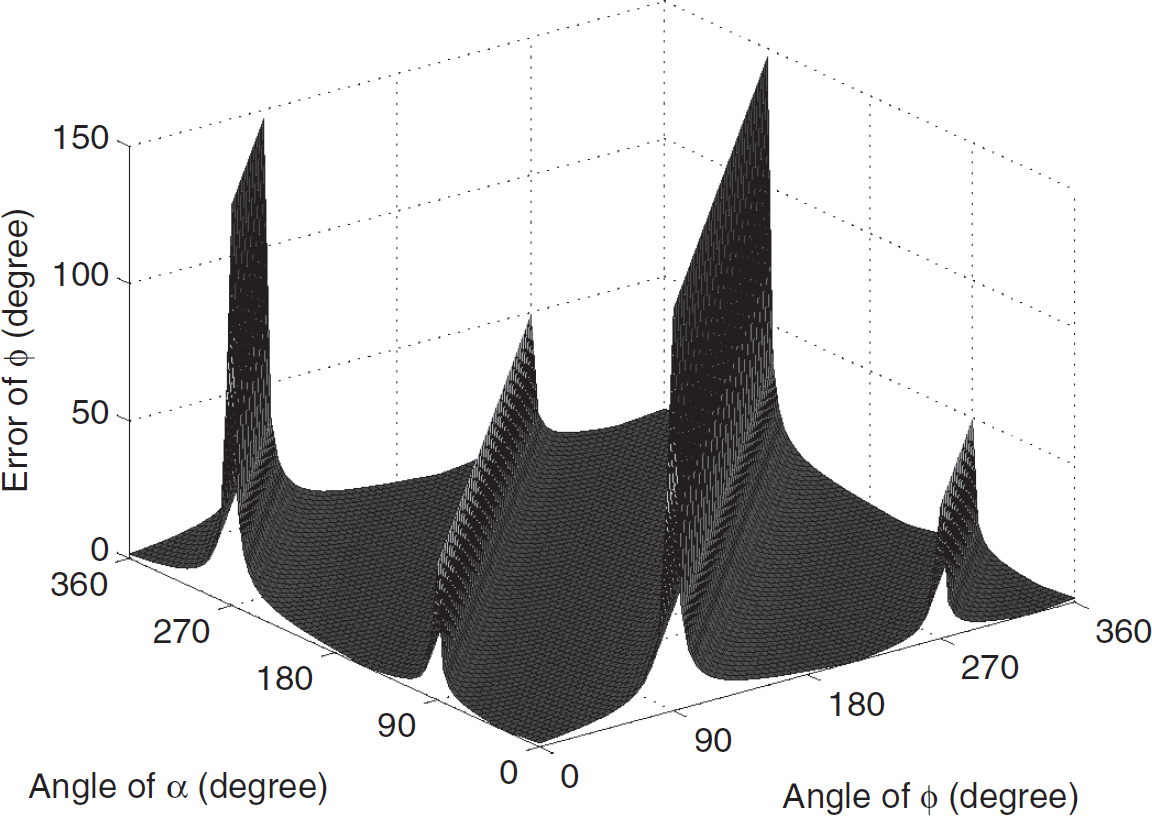
Error in computed ϕ of the original CPA algorithm.

Figure 4.

Contour of the computed f error in the original CPA algorithm.

If there are only errors in sensors location, we obtain:

| Δ ϕ | = | \frac{Δ r_{3 k}}{r_{3 k}} | \cdot | \frac{a_{1} \cdot \cos ϕ - a_{2} . \sin ϕ}{a_{1} \cdot \sin ϕ + a_{2} . \cos ϕ} |

(27)

where $| \frac{Δ r_{3 k}}{r_{3 k}} |$ is the normalized error in the measurement of r_3k as a fraction of the length of r₃k. If δ = 0.1 sec, Δr_3k = 2 m, r_3k = 40 m and the target velocity is 10 m/s, then the average error (given angle α and ϕ change from 0° to 360°) in computing ϕ caused by the error in the measured CPA times is 0.112. The average error caused by the uncertainty of the sensor location is 0.202. Therefore, sensors location error impacts the result Δϕ more seriously than the measure CPA times.

From the above analysis, we conclude two facts. First, the computation of ϕ in the original CPA algorithm is still useful because with certain network configurations (e.g., (α - ϕ) ≈ arcsin(v · δ/Δr_3k)), the error in computing ϕ is very small. For example, as shown in Fig. 4, when α = 120° and ϕ = 87°, the error in computing ϕ is 0.068°. In fact, this is one of the network configurations we used in the field experiments where the results show a small error in the computing ϕ. Second, we notice that the error in ϕ is inversely proportional to r_3k, so the node that is farthest from n₀ should be selected as node n_k. On the other hand, the error in ϕ is also related to the angle α - ϕ. Therefore, to minimize the error in computing ϕ, a trade-off between the node distance r_3k and angle (α - ϕ) must be considered. From Eq. (25), by neglecting the impact of measured CPA times, we obtain:

Δ ϕ = Δ r_{3 k} \cdot \tan (α - ϕ) / r_{3 k}

(28)

By minimizing the right part of this equation, a proper node n_k can be found for calculating ϕ.

3.3. Enhanced CPA (ECPA) Algorithm

From the above discussions, we have shown the poor performance of the original CPA algorithms in calculating target location and trajectory direction using wireless sensor networks because of two main reasons. First, it must know the network configuration in advance, i.e., how the trajectory divides the group of sensors. For the CPA algorithm in [1], four nodes must be unevenly divided by the trajectory (three on one side and one on the other side), whereas for that in [2], three nodes are to be located at the same side of the target trajectory. In a realistic system, it is impossible to know the network configuration before the target traverse the sensor field. On the other hand, the CPA localization algorithm needs such information to perform correctly. Second, as stated in Section 3.2.1, the uncertainty of sensor location and measured CPA times can cause huge errors in computing target location.

To address these issues, we proposed the enhanced CPA (ECPA) algorithm. It first determines the network configuration by estimating the trajectory slope and location. From these estimates, we can determine whether the error in computing ϕ will be small or large (Fig. 3). If the error is small, then four possible values of ϕ are calculated using the original CPA algorithm and the one that is closest to the estimated value will be chosen as the correct ϕ. However, if the network configuration causes huge errors (e.g., |α - ϕ| = 90°), the ECPA algorithm adopts the estimated ϕ as the correct angle. Finally, the trajectory is located based on the received signal strength at node n₀ and n_k where n_k is the closest node to n₀. To check the robustness of the ECPA algorithm, an analysis of the localization error is stated as well.

3.3.1. Estimating Trajectory Slope and Location

For determining the network configuration, we first estimate the trajectory slope based on the CPA time measurements, and then the trajectory location from the received signal strength at two sensors which are farthest from the trajectory.

To estimate the trajectory slope, we select five sensors that are intersected by the trajectory of the target. This assumption is satisfied if the area traversed by the target is covered by a sufficient number of sensors [20], so that a set of five sensors triggered by the target can be selected, e.g., those five on the convex hull of triggered sensors, such that they are also intersected by the target trajectory. The original CPA algorithm requires at least three nodes to be on the same side of the target trajectory, so no matter where the trajectory is located this condition must always hold if there are five nodes. The two nodes of the five with the earliest and latest measured CPA times are selected and denoted as n₁ and n₃, respectively. And n₂ is the node that is located farthest from the line n₁n₃, as shown in Fig. 5. Assume that the slope of the target trajectory is −1/k. Then the slope of line l (which is orthogonal to the trajectory) is k. Thus the formula of line l is:

l : k \cdot x - y + (y_{n_{2}} - k \cdot x_{n_{2}})

(29)

Figure 5.

Estimating the Slope of Target Trajectory.

The distance from node n₁ and n₃ to the line l is:

d i s_{i} = \frac{| k \cdot x_{n_{i}} - y_{n_{i}} + (y_{n_{2}} - k \cdot x_{n_{2}}) |}{\sqrt{k^{2} + 1}} (i = 1, 3)

(30)

Since the target is moving at a constant speed, the ratio between dis₁ and dis₃ should be equal to:

| (t_{2} - ζ_{2}) - (t_{1} - ζ_{1}) | / | (t_{3} - ζ_{3}) - (t_{2} - ζ_{2}) |

(31)

where t_i is the measured CPA time at node n_i, ζ_i is the time of sound propagation from the closest point of approach (CPA) of node n_i to its position $(x_{n_{i}}, y_{n_{i}})$ . It can be further rewritten as:

| (t_{2} - t_{1} + ζ_{1} - ζ_{2}) | / | (t_{3} - t_{2} + ζ_{2} - ζ_{3}) |

(32)

Compared to the speed of sound c, the target velocity v in our system is very small, i.e. v ≪ c. Thus, we obtain dis₁/dis₃ ≈ |(t₂ - t₁)|/|(t₃ - t₂)| because ζ₁ - ζ₂ ≪ t₂ - t₁ and ζ₂ - ζ₃ ≪ t₃ - t₂. Therefore, we have:

\frac{k \cdot x_{n_{1}} - y_{n_{1}} + (y_{n_{2}} - k \cdot x_{n_{2}})}{k \cdot x_{n_{3}} - y_{n_{3}} + (y_{n_{2}} - k \cdot x_{n_{2}})} \approx \frac{| t_{2} - t_{1} |}{| t_{3} - t_{2} |}

(33)

After solving the above formula, two possible values of k are obtained. Since line l must be located between line n₂n₁ and n₂n₃, we can easily eliminate one and select the correct k. Therefore, the estimated slope of the target trajectory is −1/k.

To estimate the trajectory location, we select those two sensors, n₁ and n₂ (different nodes from the previous example), with the smallest received signal amplitude, i.e., they are at the farthest position from the trajectory.

Suppose the estimated slope of the trajectory is k′, then we have:

d i s_{i} = \frac{| k^{'} \cdot x_{n_{i}} - y_{n_{i}} + b |}{\sqrt{k^{'} + 1}} (i = 1, 2)

(34)

Since the distance dis_i is roughly inversely proportional to the square root of the received signal amplitude, we can solve Eqs. (34) to get two possible values of b that denote two possible locations of the trajectory.

Because n₁ and n₂ can be either on the same or different sides of trajectory, we have two possible network configurations as shown in Fig. 6a and Fig. 6b. In this figure, the two possible trajectories l (the correct one) and l′ (the wrong one) are shown as solid and dashed lines, respectively. In Fig. 6a where n₁ and n₂ are on the same side of the trajectory, if l′ is considered the expected trajectory, it will contradict the assumption that both n₁ and n₂ are at the farthest position. In Fig. 6b where n₁ and n₂ are on different sides, line l′ denotes the trajectory outside the convex hull of sensors which also contradicts the assumption that the trajectory intersects the convex hull. Eliminating the inadmissible solutions, we eventually derive an approximate formula for target trajectory in the coordinate system.

Figure 6.

Estimating the location of target trajectory.

Although the estimated trajectory location is not accurate enough to meet our target localization goal (i.e., the localization error is smaller than 3 m), it is sufficient for determining how sensors are divided by the trajectory. Of these five sensors, there are always four that meet the configuration requirement and will be chosen to provide inputs to the original CPA algorithm.

3.3.2. Computing the Exact Trajectory

The ECPA algorithm considers the estimated direction (slope) of the trajectory obtained from the previous section as a reference to select the exact ϕ from those four possible values. The trajectory is then recomputed based on this newly computed slope and the received signal strength at the sensors.

Since there are four sensors meeting the requirement of the original CPA algorithm, the target velocity and the four possible directions of the trajectory can be readily calculated. Based on the approximate trajectory, four sensors are divided into two groups: one is on one side and the other three on the other side. Then, from Eq. (18), the Mach number M can be computed. Inserting M into Eq. (19), together with cos $cos ϕ = \pm \sqrt{1 - {sin}^{2} ϕ}$ , we obtain four possible values of ϕ. At this step, node n_k used in the computation must meet the condition min {Δr_3k · tan(α - ϕ)/r_3k}. However, because the uncertainty of the node positions and measured CPA times can cause r to be incorrectly computed, it is difficult to verify the correct ϕ by the incorrectly calculated r. As it will be shown in Section 4, the failure rate of the original CPA algorithm is very high (about 90%) because of the huge error in computing r. Therefore, in the ECPA algorithm, the approximate ϕ serves as the reference, and the ϕ that is closest to the estimated one will be considered the correct result. This comparison process needs to be done only for some specific network configurations, whereby α and ϕ are located within the white region in Fig. 4. Otherwise, the estimated ϕ will be used as the final result. Our simulations confirm that this scheme can generate very small errors of the trajectory direction (less than 6° from the actual value).

To calculate the trajectory location, we make use of the newly computed slope of the trajectory and the received signal strength at the sensors. Suppose node n_k is the closest one to node n₀ and the square root of the received signal amplitude at node n₀ and n_k are s₀ and s_k, respectively. As shown in Fig. 7, we have r/h = r₁/h₁ = s_k/s₀, so r₁ can be calculated from the following equation:

r_{1} \cdot s_{0} = (r_{k} - r_{1}) \cdot s_{k}

(35)

where r_k is the distance between node n₀ and n_k. After obtaining r₁, we can easily locate the target trajectory and compute r as well. Although the received signal strength at the nodes may be affected by several environmental factors, it does not influence the result as significantly as the errors of sensors location and measured CPA times. This result will be shown in the next section. Furthermore, as it will be shown in our simulations and experimental results, the target localization errors are very small in the ECPA algorithm (less than 2 m).

Figure 7.

The computation of distance r1 in ECPA algorithm.

3.3.3. Sensitivity of Distance Computation in the ECPA Algorithm

An important issue associated with the ECPA algorithm is how sensitive it is to errors in the input parameters. The robustness of the method requires that small errors in the input will not result in huge errors in the results. To see under what conditions our method is robust, we study the sensitivity of the computation of r₁. Since r₁ ≥ r, the error in computed r₁ can be considered as the upper bound of error in r.

In Eq. (35), the input parameters include r_k, s₀ and s_k. Small changes in r_k, s_k, and s₀ yield a small change in r₁ as follows:

Δ r_{1} = \frac{s_{k} \cdot Δ r_{k} + r_{k} \cdot Δ s_{k} + r_{1} \cdot Δ S_{k} - r_{1} \cdot Δ s_{0}}{s_{0} + s_{k}}

(36)

Assuming s_k ≤ s₀, then the above formula yields:

Δ r_{1} \leq 0.5 \cdot Δ r_{k} + 0.5 \cdot r_{k} \cdot e_{k}

(37)

where Δr_k is the average error in the sensors location, e_k = (Δs_k)/s_k is the percentage error in received signal strength at node n_k. If s_k > s₀, the same formula applies except that e_k = (Δs₀)/s₀. Figure 8 shows that the localization error, where the x-axis is the distance between node n₀ and n_k and the y-axis is the percentage error in the received signal strength at sensors. The maximal error in computed r₁ is about 6 m, when the distance to node n_k is 20 m and RSSI error is 50%. Compared to the original CPA algorithm, as shown in Fig. 2, the ECPA algorithm generates a smaller error in locating the target trajectory.

Figure 8.

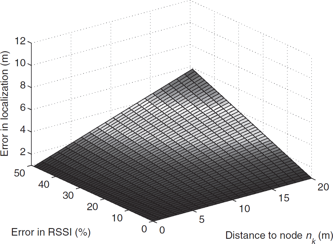
Error in the computed r of the ECPA algorithm.

From Eq. (37), we notice that the upper bound of error in the computation of r₁ is roughly proportional to (r_k · e_k) since 0.5 · Δr_k is a small constant and can be omitted. Therefore, to achieve a smaller localization error, the distance between the triggered sensors should not be too large, which is often the case in most wireless sensor network deployments since the detection range of sensors is quite limited.

Though it is hard to reduce the error in e_k, we can choose the node with a shorter distance to n₀ as n_k to decrease the error in computed r₁. For instance, given a typical case, where r_k = 20 m, Δr_k = 2 m and c_k = 20%, then the error in computed r₁ will be bounded within 3 m.

In summary, the ECPA algorithm is different from the original CPA algorithm in four aspects. First, the ECPA algorithm can determine the network configuration by itself, which is impossible in the original CPA algorithm. Second, in calculating ϕ, the ECPA algorithm selects the optimal sensors to minimize the computation error, but the original CPA algorithm arbitrarily chooses one. Third, the ECPA algorithm uses the estimated ϕ as the reference to choose the correct value of ϕ while CPA fails to do so because of the huge error in computing r. Fourth, the received signal strength at the sensors is used to calculate the target trajectory instead of the measured CPA times because a small error in measured CPA times can result in a huge error in the computation of r, as proven in Section 3.2.1. To further verify our design, the ECPA algorithm was implemented in both simulations and field experiments as described in the following sections.

4. Experimental Setup and Issues

In this section, we describe the framework of our target detection, localization, and tracking system and the details of the architecture, hardware information, internetworking mixed networks, and target detection method.

4.1. System Architecture

Our target detection and tracking system is composed of six components that are inter-networked together using either IEEE 802.11 or IEEE 802.3, and directed diffusion [21]. Although we currently use only one cluster to demonstrate that the concept is practical, our goal is to eventually extend it to larger networks by adopting multiple clustering algorithms for target tracking, such as [22, 23].

Each of the six components represents a role or a function which is performed by one or multiple computers. Fig. 9 illustrates the architecture of the system. The six components are as follows:

sensor nodes that monitor for targets, detect the measured CPA time, and report results to the cluster head through the directed diffusion network,

cluster head node that receives the CPA time data from sensors over the directed diffusion sensor network as the input to determine the position, direction, and velocity of the target by running the ECPA algorithm,

the gateway node that internetworks the diffusion network to the IP network,

camera control node that receives packets from the gateway, and then predicts the target position based on the target velocity and the time delay for package transmission from the sensors to the camera control node,

video capture node that is responsible for interfacing with the video output of the camera,

system control node that manages the execution of the remote nodes. For detailed descriptions of the experiment setup, please refer to [24].

Figure 9.

System Architecture for Collaborative Mixed Wireless Sensor Networks.

4.2. Hardware

Each of the nodes is an x86-based laptop computer. The sensor nodes including the cluster head are laptops with 800 MHz CPU and 82801CA/CAM AC'97 Audio Controllers. The gateway node, camera control, and system control are laptops with 1.2 GHz CPU and 512 MB memory. The video capture computer is a Pentium IV based laptop (1.2 GHz CPU) with Windows XP operating system. Each computer is also equipped with an IEEE 802.11b card for wireless connectivity. Video capture is performed using a Pinnacle 500 USB video converter which converts the camera's RCA output to digital video and interfaces with the computer using USB 2.0. The camera is a Sony EVID30, and the interface to the controller is RS232C, 9600 bps, serial port.

4.3. Internetworking Mixed Networks

The target tracking system is networked using several different network technologies. The sensors and cluster head communicate through directed diffusion running over an 802.11 network. The camera control and system control machines are connected with an 802.3 (Ethernet) network running IP. In order to internetwork the two networks we developed an internetworking software which executes on the gateway node. The gateway is configured with both an 802.11 interface and an Ethernet interface. The internetworking software converts diffusion packets into IP packets and vice versa.

4.4. Target Detection and Time Sychronization

A typical recorded sound (5 sec long) of the moving vehicle with a sample rate of 4 kHz is shown in Fig. 10. The CPA time can be obtained as the instance when the highest amplitude occurs which is indicated by a vertical line in Fig. 10. Obviously, longer recording times will cause higher detection delays, so the recording time should be as short as possible.

Figure 10.

A typical audio recording of the moving vehicle.

Time synchronization among sensor nodes was achieved by NTP (Network Time Protocol), which synchronizes the clocks of sensors over packet-switched, variable-latency wireless networks. NTP typically provides accuracies of less than a few milliseconds on wireless networks [25], which is accurate enough for the ECPA algorithm to successfully localize the target.

5. Experimental Results

To evaluate the performance of our systems, we set up the target detection and tracking sensor networks at two field locations: a vacant parking lot at Auburn University, as shown in Fig. 11 and at AU's National Center for Asphalt Technologies (NCAT) test tracks. We experimented with several wireless ad-hoc sensor network configurations:

a basic sensor network and camera network configuration,

a network with 3 additional wireless network hops from the cluster head to the camera control node and

a network that allows more directions (orientations) for the target to move.

Figure 11.

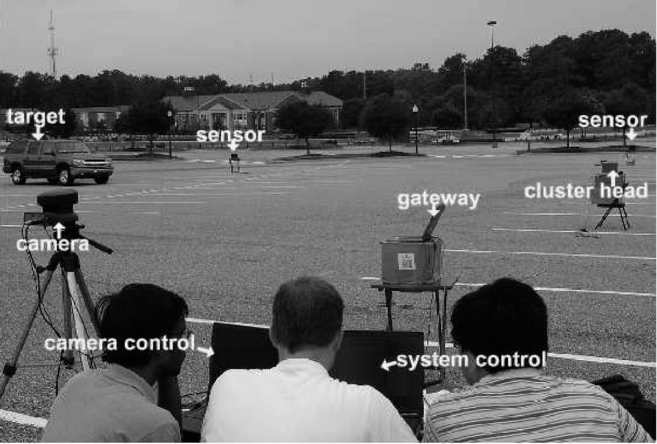
Experimental setup for target tracking in a vacant parking lot at Auburn University.

5.1. Results of Computing Target Location and Velocity

The ECPA algorithm computes the target location, velocity, and direction of travel based on the CPA time reported from the five sensors. Table 1 summarizes the results of the eight runs that we conducted with two target trajectories. The results show that the target location and velocity can be accurately computed. The average position error is only 1.8 meters, the average velocity error is only 3 mph, and the average trajectory error is 5 degrees. For example in the first run, the predicted target location is (3608558, 641360), only 1 m from the actual location (3608558, 641359). The computed speed is 28 mph whereas the actual speed is 30 mph, and the direction of travel is 90 degrees compared to the actual direction of 87 degrees.

TABLE 1
Tests Results

Target Position (m) Speed (mph) Angle (degree)

Run Computed Error Computed Error Computed Error

1st (3608558, 641360) 1 28   2   90 3

2nd (3608558, 641360) 1 27   3   90 3

3rd (3608559, 641357) 2.236 42 12   84 3

4th (3608552, 641359) 6 27   3 111 24

5th (3608545, 641358) 1 29   1 127 1

6th (3608544, 641359) 1 28   2 130 2

7th (3608544, 641359) 1 29   1 131 3

8th (3608545, 641360) 1 32   2 132 4

Min Error 1 1     1

Max Error 6 12   24

Avg Error 1.78   3.25             5.375

	Target Position (m)	Speed (mph)	Angle (degree)
Run	Computed	Error	Computed	Error	Computed	Error
1st	(3608558, 641360)	1	28	2	90	3
2nd	(3608558, 641360)	1	27	3	90	3
3rd	(3608559, 641357)	2.236	42	12	84	3
4th	(3608552, 641359)	6	27	3	111	24
5th	(3608545, 641358)	1	29	1	127	1
6th	(3608544, 641359)	1	28	2	130	2
7th	(3608544, 641359)	1	29	1	131	3
8th	(3608545, 641360)	1	32	2	132	4
Min Error	1		1		1
Max Error	6		12		24
Avg Error	1.78		3.25		5.375

Figure 12 shows the predicted position and actual path of the vehicle for the eight runs in our experiments. Note that the computed target trajectories almost exactly match the actual values. The shorter dashed lines show the results from two runs in the AC direction and two runs in the CA directions. These trajectories are very close to the actual one shown by the solid AC path. The longer dashed lines show the results of two runs in the BD direction and two runs in the DB direction. These trajectories (with one exception) are very close to the actual trajectory.

Figure 12.

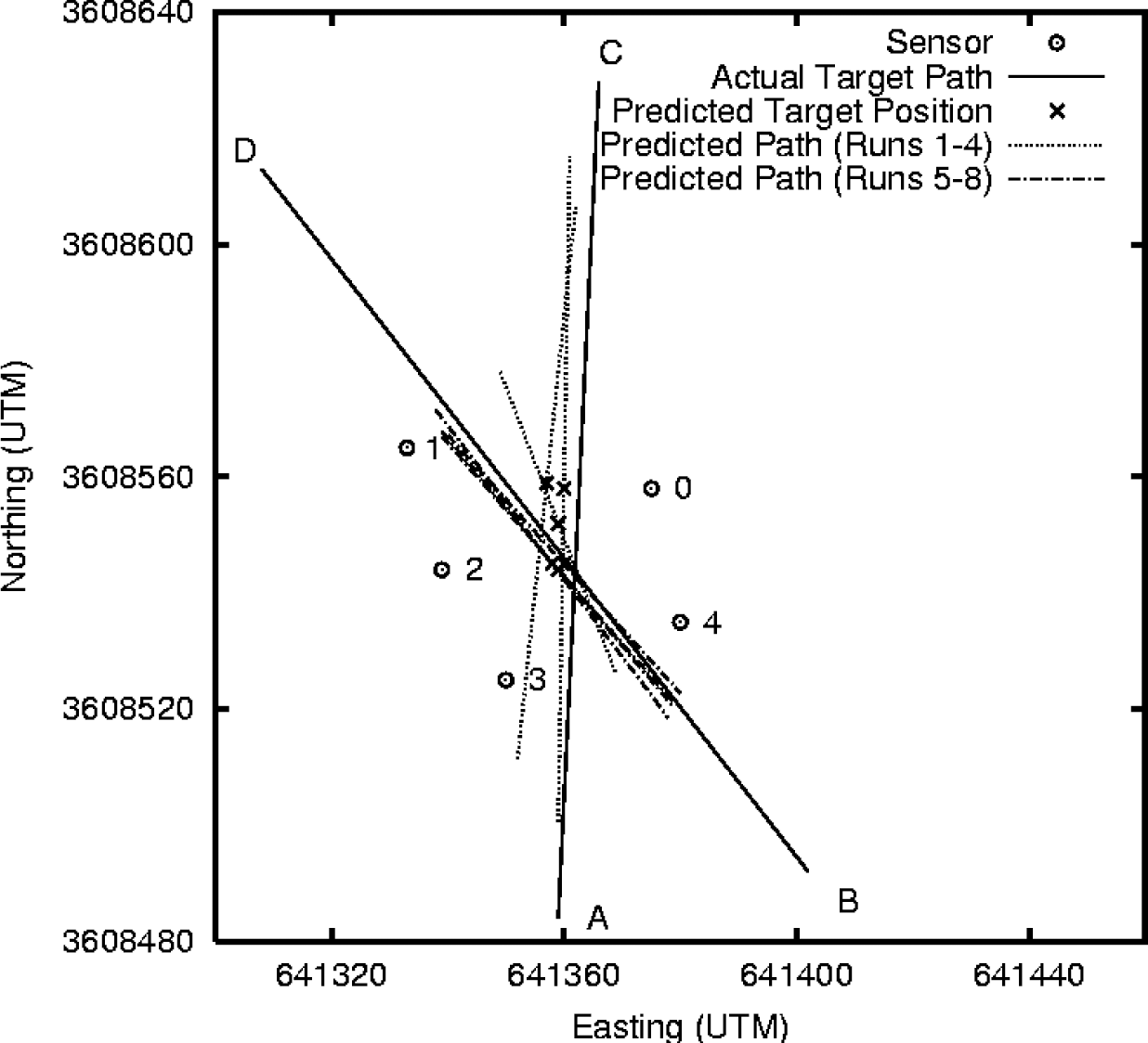
Plot of target tracking results showing computed target location and velocity match the actual value.

Compared to the results published in [5], the ECPA algorithm gives more accurate results. For example, the average localization error in the ECPA algorithm is 1.78 m; while the root mean square errors of Extended Kalman Filter (EKF), Lateral Inhibition (LAT), and EKF & LAT are 8.877 m, 9.362 m, and 11.306 m, respectively.

6. Simulation and Results

To further study the impact of target velocity and location errors on localization and velocity errors, we use an extended ns-2 simulation tool (ns-2.27), from the Naval research laboratory [26]. It provides simulation models for various physical phenomena such as acoustic, seismic, and chemical agents. The presence of physical phenomena in ns-2 is modeled with broadcast packets which are sent over a designated channel called the “phenom” channel. In the real world, detecting acoustic events is made more difficult by the environmental noise and sensitivity issues of the microphones. We assume that the acoustic packets experience a loss profile similar to 802.11 data packets, so the noise and packet losses are simulated by the extensions provided in [27]. In the simulation, we use the same node deployment as was used in the field experiment. As expected, the simulation results with target velocities of 30mph, match the field-test very well.

6.1. Successful Localization Rate

Due to the error in measured CPA time, the original CPA algorithm always fail to select the proper ϕ value. In most cases, the CPA algorithm can find r > 0, but after inserting this r into the CPA algorithm, the resulting trajectory is outside the convex hull of the sensors. Thus, the localization process failed. As shown in Fig. 13, the successful detection rate of CPA is at most 10%. Furthermore, when considering the error in a sensor location, the situation becomes even worse. The ECPA algorithm, however, first chooses the ϕ which is closest to the estimated one, and then maps the trajectory into the convex hull of the sensors, thereby achieving a localization success rate of 100%.

Figure 13.

Successful Localization Rate of ECPA and CPA Algorithms.

6.2. Impact of Velocity

As described in [1], the relative error on the target distance estimate is roughly inversely proportional to the square root of the Mach number. This means the localization error in the ECPA algorithm should also decrease as the target velocity increases. This property is demonstrated in Fig. 14, where the average velocity error decreases from 1.3 m/s to 0.2 m/s, average direction error decreases from 5.5° to 0.5° and the average location error decreases from 1.35 to 0.7 meters. Note that when the target speed is 13 m/s (30mph), the error in estimated location, velocity and direction are 1 m, 1.7 mph and 3.5°, respectively. Indeed, these values are very similar to the errors experienced in the field (Table 1).

Figure 14.

Impact of different target velocity on the ECPA algorithm.

6.3. Impact of Sensors Location Errors

Errors in sensor location range from less than one meter to a few meters, depending on the localization technology. To understand the effect of this error, we simulated sensors location error as a uniform distributed function upon (0, max], where max increases from 0.1 to 5 meters. As shown in Fig. 15, when the location error in sensors increases, the target localization error also increases. Interestingly, the ECPA algorithm is highly tolerant of the sensors location error because the estimated target information is quite close to the actual values even with a larger sensor location error. For example, when maximal sensors location error is 5 meters, the average error in target location is only about 1.8 meters. This result matches the mathematical analysis, since Δr ≈ 0.5 · Δr_k where Δr_k = 2.5 m. Moreover, the error in the estimated velocity and direction are still within the acceptable range (0.8 m/s and 6°).

Figure 15.

Impact of sensors location errors on the ECPA algorithm.

6.4. Impact of Distance Between Sensors

To evaluate the impact of different distances between sensors on localization errors, we simulated a set of nodes deployment which covered difference sizes of area in the networks. The area covered by the sensors is defined as the size of convex hull of the sensors. As shown in Fig. 16, when the size of the covered area increases, the errors in calculating the velocity, direction, and position of the mobile target also increase. This is mainly because the longer distance between the sensors and the target trajectory causes huge errors in the measurement of the CPA times. These errors significantly affect the results. As previously stated in our sensitivity analysis of the ECPA algorithm, a larger distance between sensor n₀ and n_k could generate larger errors in locating the trajectory. This fact is again verified in the simulation results, as shown in Fig. 16c. Although larger distances between sensors could cause some problems, the errors in the computed target velocity, direction, and position are still acceptable (4 m/s, 10° and 4 m, respectively).

Figure 16.

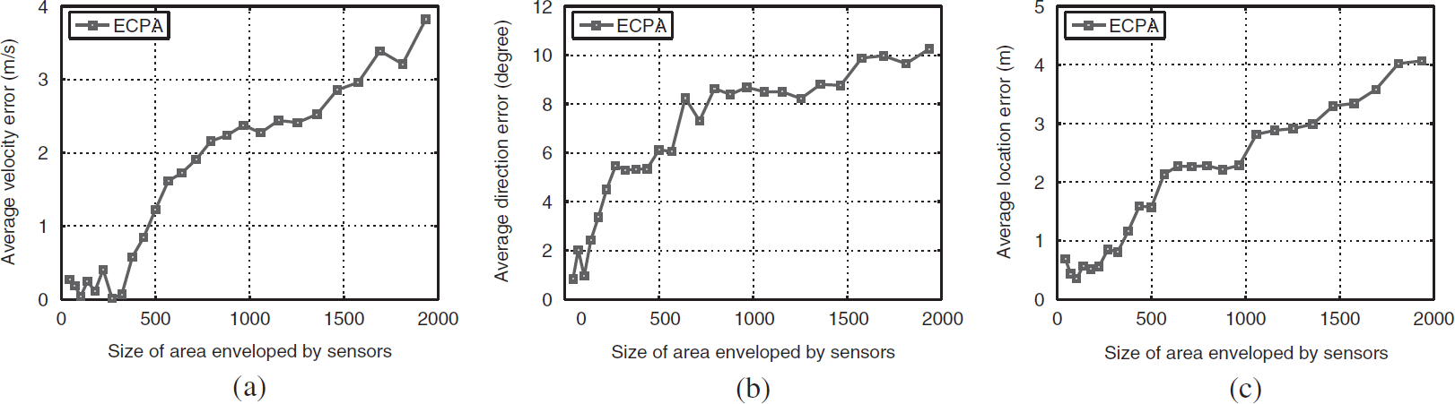
Impact of different distance between sensors on the ECPA algorithm.

7. Conclusion

The original CPA algorithm fails because the uncertainty of sensors position causes it to fail to obtain a positive value of r (distance between a target and the reference node). Our enhanced CPA scheme first estimates the trajectory and obtains the sensors deployment information. Then, it selects the optimal four sensors to minimize the computation error in ϕ with the original CPA algorithm. Finally, the trajectory location is calculated based on the newly computed angle and received signal strength at sensors. Through our field experiments, we have shown that the ECPA algorithm is an efficient and practical localization and tracking method for moving vehicles using wireless sensor networks.

For rapid deployment in the field, we will design new compact sensor fusion nodes based on COTS components (such as PC104), which are small, inexpensive, and can execute collaborative algorithms for reliably detecting and tracking targets. In addition, we will extend the network to multiple clusters to enable us to track targets moving along nonlinear paths. Finally, we will experiment with arbitrary deployment of sensors in random configurations and develop methods for automatically forming clusters in these topologies.

Our prototype target tracking system demonstrates the feasibility of detection, tracking, and image/video capture of moving targets using collaborative, wireless, acoustic sensor nodes. By using the ECPA localization algorithm, the target position, velocity, and direction can be accurately computed and transmitted to the video camera.

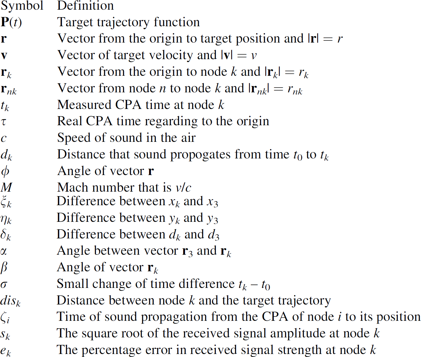
Nomenclature

Symbol	Definition
P(t)	Target trajectory function
r	Vector from the origin to target position and \|r\| = r
v	Vector of target velocity and \|v\| = v
r_k	Vector from the origin to node k and \|r_k\| = r_k
r_nk	Vector from node n to node k and \|r_nk\| = r_nk
t _k	Measured CPA time at node k
τ	Real CPA time regarding to the origin
c	Speed of sound in the air
d _k	Distance that sound propogates from time t₀ to t_k
ϕ	Angle of vector r
M	Mach number that is v/c
ξ _k	Difference between x_k and x₃
η _k	Difference between y_k and y₃
δ _k	Difference between d_k and d₃
α	Angle between vector r₃ and r_k
β	Angle of vector r_k
σ	Small change of time difference t_k - t₀
dis _k	Distance between node k and the target trajectory
ζ _i	Time of sound propagation from the CPA of node i to its position
s _k	The square root of the received signal amplitude at node k
e _k	The percentage error in received signal strength at node k

References

Dommermuth

F. M.

, “The estimation of target motion parameters from cpa time measurements in a field of acoustic sensors,” The Journal of the Acoustical Society of America, vol. 83, no. 4, pp. 1476–1480, 1988.

Milios

E. E.

Nawab

S. H.

, “Acoustic tracking from closest point of approach time, amplitude, and frequency at spatially distributed sensors,” The Journal of the Acoustical Society of America, vol. 87, no. 3, pp. 1026–1034, 1990.

Zhao

Shin

Reich

, “Information-driven dynamic sensor collaboration,” Signal Processing Magazine, IEEE, vol. 19, no. 2, pp. 61–72, March 2002.

Wong

K. D.

Y. H.

Sayeed

A. M.

, “Detection, classification and tracking of targets in distributed sensor networks,” Signal Processing Magazine, IEEE, vol. 19, no. 2, pp. 17–30, March 2002.

Brooks

Ramanathan

Sayeed

, “Distributed target classification and tracking in sensor networks,” Proceedings of the IEEE, vol. 91, no. 8, pp. 1163–1171, Aug. 2003.

Brooks

R. R.

Griffin

Friedlander

, “Self-organized distributed sensor network entity tracking,” International Journal of High Performance Computing Applications, vol. 16, no. 3, pp. 207–219, 2002.

Ercan

A. O.

Gamal

A. E.

Guibas

L. J.

, “Object tracking in the presence of occlusions via a camera network,” in IPSN ′07: Proceedings of the 6th International Conference on Information Processing in Sensor Networks New York, NY, USA: ACM, 2007 pp. 509–518.

Ali

A. M.

Yao

Collier

T. C.

Taylor

C. E.

Blumstein

D. T.

Girod

, “An empirical study of collaborative acoustic source localization,” in IPSN ′07: Proceedings of the 6th International Conference on Information Processing in Sensor Networks. New York, NY, USA: ACM, 2007 pp. 41–50.

Singh

Madhow

Kumar

Suri

Cagley

, “Tracking multiple targets using binary proximity sensors,” in IPSN ′07: Proceedings of the 6th International Conference on Information Processing in Sensor Networks New York, NY, USA: ACM, 2007 pp. 529–538.

10.

Shrivastava

Madhow

R. M. U.

Suri

, “Target tracking with binary proximity sensors: fundamental limits, minimal descriptions, and algorithms,” in SenSys ′06: Proceedings of the 4th International Conference on Embedded Networked Sensor Systems New York, NY, USA: ACM, 2006 pp. 251–264.

11.

Kim

Mechitov

Choi

J.-Y.

Ham

, “On target tracking with binary proximity sensors,” in IPSN ′05: Proceedings of the 4th International Symposium on Information Processing in Sensor Networks Piscataway, NJ, USA: IEEE Press, 2005 p. 40.

12.

Yang

, “Cooperative target localization method for heterogeneous sensor networks,” in ICCNMC05: International Conference on Computer Networks and Mobile Computing, 2005 pp. 13–22.

13.

Brooks

R. R.

Iyengar

S. S.

, “Multi-Sensor Fusion: Fundamentals and Applications with Softwares,” Upper Saddle River, NJ, USA: Prentice-Hall, Inc., 1998.

14.

Sheng

Y. H.

, “Energy based acoustic source localization,” in IPSN ′03: Proceedings of the 6th International Conference on Information Processing in Sensor Networks, 2003 pp. 285–300.

15.

Sheng

Y.-H.

, “Maximum likelihood multiple-source localization using acoustic energy measurements with wireless sensor networks,” Signal Processing, IEEE Transactions on, vol. 53, no. 1, pp. 44–53, 2005.

16.

Rao

Sastry

Zhou

, “Tracking the direction of arrival of multiple moving targets,” Signal Processing, IEEE Transactions on, vol. 42, no. 5, pp. 1133–1144, May 1994.

17.

Boettcher

P. W.

Shaw

G. A.

, “Energy-constrained collaborative processing for target detection, tracking, and geolocation,” in IPSN ′03: Proceedings of the 6th International Conference on Information Processing in Sensor Networks, 2003 pp. 254–268.

18.

Boettcher

P. W.

Sherman

J. A.

Shaw

G. A.

, in Target Localization using Acoustic Time-Difference of Arrival in Distributed Sensor Networks, Suresh

Roper

W. E.

, Eds., vol. 4741, no. 1. SPIE, 2002 pp. 180–191.

19.

Intanagonwiwat

Govindan

Estrin

, “An error model for sensor simulation gps and differential gps,” in Position Location and Navigation Symposium, IEEE, April 1994 pp. 260–266.

20.

Wang

Xing

Zhang

Pless

Gill

, “Integrated coverage and connectivity configuration in wireless sensor networks,” in SenSys ′03: Proceedings of the 1st International Conference on Embedded Networked Sensor Systems New York, NY, USA: ACM, 2003 pp. 28–39.

21.

Silva

Heidemann

Govindan

, “Network routing application programmer's interface,” 2002 [Online]. Available: citeseer.ist.psu.edu/silva02network.html.

22.

Neelisetti

Lim

Agrawal

Yang

, “A robust clustering algorithm for target tracking in wireless acoustic sensor networks,” in IRA-DSN 2007: Innovations and Real-time Applications of Distributed Sensor Networks (DSN) Symposium, 2007 pp. 17–25.

23.

Chen

W.-P.

Hou

J. C.

Sha

, “Dynamic clustering for acoustic target tracking in wireless sensor networks,” IEEE Transactions on Mobile Computing, vol. 3, no. 3, pp. 258–271, 2004.

24.

Yang

Lim

Casey

Neelisetti

, “Real-time target tracking with CPA algorithm in wireless sensor networks,” Sensor, Mesh and Ad Hoc Communications and Networks, 2008. SECON ′08. 5th Annual IEEE Communications Society Conference on, pp. 305–313, June 2008.

25.

[Online]. Available: http://www.ntp.org/.

26.

[Online]. Available: http://cs.itd.nrl.navy.mil/work/sensorsim/index.php.

27.

Xiuchao

Ananda

A. L.

, “Link characteristics estimation for ieee 802.11 dcf based wlan,” in LCN ′04: Proceedings of the 29th Annual IEEE International Conference on Local Computer Networks Washington, DC, USA: IEEE Computer Society, 2004 pp. 302–309.

An Enhanced CPA Algorithm for Real-Time Target Tracking in Wireless Sensor Networks

Abstract

Keywords

1. Introduction

2. Related Work

3. Target Localization Algorithm

3.1. Original CPA Algorithm

3.2.1. Sensitivity of Distance Computation

3.3.1. Estimating Trajectory Slope and Location

4.1. System Architecture

4.3. Internetworking Mixed Networks

4.4. Target Detection and Time Sychronization

6.1. Successful Localization Rate

Nomenclature

References