Power Assignment for Symmetric Communication in Wireless Sensor Networks

Abstract

We show that two incremental power heuristics for power assignment in a wireless sensor network have an approximation ratio 2. Enhancements to these heuristics are proposed. It is shown that these enhancements do not reduce the approximation ratio of the considered incremental power heuristics. However, experiments conducted by us indicate that the proposed enhancements reduce the power cost of the assignment on average. Further, the two-edge switch enhancements reduce the power-cost reduction (relative to using minimum cost spanning trees) that is, on average, twice as much as obtainable from any of the heuristics proposed earlier.

Keywords

Power Assignment Symmetric Connectivity Wireless Sensor Networks Approximation Algorithm

1. Introduction

We consider the problem of assigning power levels to the sensors in a wireless sensor network so that the total power assigned is minimum and the communication graph of the sensor network has a path composed solely of bidirectional edges¹ between every pair of sensors. We assume that the sensors are battery operated and are deployed in an environment in which it is impractical (or at least undesirable) to recharge/replace the battery of a sensor (e.g., in a battlefield or at the bottom of an ocean). Hence, energy conservation is paramount. Although sensors use energy to sense as well as to communicate among themselves, our focus here is on the conservation of energy spent in communication activities. Depending on the application, inter sensor communication may be modeled as unicast, multicast, or broadcast.

We assume the omnidirectional antenna model in which the n-sensor wireless network is represented as a complete weighted directed graph G that has n vertices/nodes (we use the terms sensor, vertex, and node interchangeably). Each node of G represents a sensor of the wireless network. The weight w(i, j) of the directed edge (i, j) is the minimum power level at which sensor i must transmit if its message is to be received by sensor j. Using an omnidirectional antenna, sensor i can transmit to sensors j₁, j₂, …, j_k, by setting its power level to

max {w (i, j_{q}) | 1 \leq q \leq k}

In the most common model used for power attenuation in wireless broadcast, signal power attenuates at the rate a/r^d, where a is a media dependent constant, r is the distance from the signal source, and d is another constant between 2 and 4 [22]. So, for this model, w(i, j) = w(j, i) = c ∗ r (i, j)^d, where r(i, j) is the Euclidean distance between nodes i and j and c is a constant. In practice, however, this nice relationship between w(i, j) and r(i, j) may not apply. This may, for example, be due to obstructions between the nodes that may cause the attenuation to be larger than predicted. Also, the transmission properties of the media may be asymmetric resulting in w(i, j) ≠ w(j, i). When w(i, j) ≠ w(j, i) for some (i, j), we say that the power requirements are asymmetric. When w(i, j) = w(j, i) for all i and j, the power requirements are symmetric.

In an effort to conserve energy, each sensor u adjusts its power level to a value p(n) such that the power cost p(G)=Σu p(u) is minimum and the subgraph H of G formed by (directed) edges (u, v) such that w(n, v) ≤ p (u) is strongly connected. The resultant subgraph is called a minimum power strongly connected topology. Note that with the set power levels, sensor u can do a single-hop transmission to every sensor v for which (u, v) is an edge of H. Since H is strongly connected, every sensor can communicate with every other sensor using a multi-hop transmission.

Fig. 1(a) shows a network with 5 sensors A through E. Each circle represents the transmission range of the sensor at its center given this sensor's current power level. The example 5-sensor network may be represented by a 5-vertex complete digraph with w(i, j) being the minimum p(i) needed to transmit from i to j. Figure 1(b) shows the subgraph H of this complete digraph with the property that for every edge (u, v) in H, p(u) ≥ w(u, v). Notice that while sensor E can do a single-hop transmission to sensor D, sensor D cannot do a similar transmission to E. This is because p(E) ≥ w(E, D) = w(D, E) > p(D). Although H is strongly connected, it is asymmetric ((E, D) is an edge of H but (D, E) is not). This asymmetry in the connectivity of H poses a problem in applications where the single-hop transmission protocol requires the receiver to send an acknowledgment to its one-hop neighbor who sent the message. So, while D can receive from E, in Fig. 1(b), D cannot send a one-hop acknowledgment of this receipt back to E. To overcome this problem, we require that H contain a spanning connected subgraph comprised solely of bidirectional edges. By using only the edges in this spanning connected subgraph, all single-hop transmissions can be acknowledged by the receiver. Figure 1(c) shows a connected spanning subgraph of Fig. 1(b) that is comprised solely of bidirectional edges. The bidirectional edges are shown as undirected edges in this figure.

Figure 1.

The connectivity model (each node has the different transmission power level): (a) Sensors and their transmission rages (b) An asymmetric communication graph and (c) A symmetric subgraph of (b).

A formal statement of the problem we study in this paper is given below.

Minimum Power Symmetric Connectivity Problem (MPSC)

Input: A complete weighted undirected graph G.

Output: A power assignment p() to the vertices of G so that the power cost p(G)=Σu p(u) is minimum and the subgraph of G comprised of bidirectional (undirected) edges (u, v) such that p(u) ≥ w(u, v) and p(v) ≥ w(u, v) (equivalently, min {p(u), p(v)} ≥ w(u, v)) is a connected spanning subgraph of G.

In Section 2, we review prior research related to the MPSC problem. In Section 3, we prove that the incremental power heuristics of [17, 4] have an approximation ratio of 2 matching the approximation ratio of the MST (minimum spanning tree) heuristic of [3, 19, 4, 10]. Enhancements of these heuristics as well as to the MST heuristic are presented in Section 4. In Section 5, we present experimental results that show that our refinements result in improved performance.

2. Related Work

The minimum energy broadcast tree problem (MEBT) is related to MPSC. In MEBT, we are to assign power levels to the nodes of G so that Σu p(u) is minimum and the graph comprised of directed edges (u, v) such that p(u) ≥ w(u, v) contains a directed tree, which is rooted at a specified source node s and which includes all vertices of G. MEBT is NP-hard, because it is a generalization of the connected dominating set problem, which is known to be NP-hard [8]. In fact, MEBT cannot be approximated in polynomial time within a factor (l−∊)Δ, where ∊ is any small positive constant and Δ is the maximal degree of a vertex, unless NP ⊆ DTIME[n^{O(log log n)}] [9]. Clementi et al. [6] show that MEBT is NP-hard when edge weights equal the Euclidean distance between the nodes (sensors). Wieselthier et al. [15, 16] consider the case when w(i, j) = r ∗ r^d. They develop a fast MEBT algorithm for the case of networks that have 3 nodes (a source broadcasting to 2 other nodes). For larger networks, they propose a recursive algorithm that “makes more than 51,000 calls” when there are 10 destination nodes. Since the proposed recursive algorithm is impractical for large networks, several heuristics are proposed. Four of the proposed heuristics are greedy heuristics that scale well as the network size increases. Wan et al. [14] provide a theoretical analysis of the performance of three of the greedy heuristics proposed in [15, 16]. They show that two of the proposed heuristics (link-based minimum spanning tree and broadcast incremental power) have constant approximation ratios and a third (shortest path spanning tree) has an approximation ratio that is at least n/2 (these approximation ratios are for the case w(i, j) = c∗r^d).

Let MPAC be the MPSC problem with the relaxation that the subgraph of G defined by the assigned power levels contain a strongly connected spanning subgraph. So it is possible that (u, v) is in the subgraph (p(u) ≥ w(u, v)) and (v, u) is not in the subgraph (p(v) < w(v, u) = w(u, v)). Chen and Huang [3] have shown that MPAC is NP-hard for general graphs. The proof of [3] applies also to MPSC. An approximation algorithm that is based on minimum cost spanning trees and that has approximation ratio 2 also is developed in [3]. This approximation algorithm appears to have been rediscovered many times by several researchers [19, 4, 10]. Kirousis et al. [10] show that MPAC is NP-hard when the edge weights are equal to distances in 3-dimensional space (E³) and Clementi et al. [7] prove this for distances in 2-dimensional space (E²).

Calinescu et al. [19] show that for a given G, the total power in the optimal solution for MPAC can be half that for the optimal solution for MPSC when the distances are in E². They develop also two approximation algorithms for MPSC. One is a fully polynomial time approximation scheme whose approximation ratio is 1 + ln 2 + ∊ and the other is a greedy algorithm whose approximation ratio is 15/8. Althaus et al. [17] establish lower approximation ratios of 5/3 + ∊ and 11/6, respectively, for the two approximation algorithms of [19]. An integer linear programming formulation for MPSC is developed in [17]. Using this formulation, MPSC instances with up to 40 sensors can be solved in about 1 hour of time on a 600MHz PC. [17] asserts that the 5/3 + ∊ algorithm is not practical and that the 11/6 algorithm, which is known as the greedy fork contraction algorithm, does not perform as well on real data as an extended minimum spanning tree algorithm EFS (edge and fork switching) that begins with a minimum cost spanning tree and iteratively reduces the power cost of this spanning tree. In each iteration, EFS finds the maximum reduction in power possible by switching a tree edge and a non-tree edge as well as by switching a fork (two non-tree edges that share a vertex) and two tree edges. The switch must leave behind a spanning tree. If the maximum reduction is positive, the switch is made and we proceed to the next iteration. Otherwise, EFS terminates. [17] also shows that approximation of MPSC with asymmetric power requirements, is NP-hard for any approximation ratio (1 − ∊) In n, where n is the number of nodes and ∊ > 0 is any constant. Cheng et al. [4] show that MPSC is NP-hard with edge weights equal to distances in E². They propose an incremental power greedy heuristic for MPSC and demonstrate experimentally that this greedy heuristic performs better than the MST-based heuristic whose approximation ratio is 2.

3. Analysis of Incremental Power Heuristics

Two incremental power heuristics have been proposed to construct minimal energy/power broad-cast trees [17, 4, 5, 15, 16]. Both heuristics are suitable for the MEBT and MPSC problems. We describe these two heuristics in the context of the MPSC problem. Conceptually, the two heuristics are identical to the well known Kruskal and Prim algorithms to construct minimum cost spanning trees [12]. In both heuristics we construct a spanning tree of the given graph G by starting with TE = Ø and adding edges to TE, one at a time, until TE becomes a spanning tree of G. At any time in the tree construction, the current power level for each vertex u is max {w(u, v)| (u, v) ∊ TE}. The next edge for inclusion into TE is the one that increases the sum of power levels the least and that creates no cycle in TE. When the spanning tree construction is complete, the p(u)s are such that the constructed spanning tree is a subgraph of the communication graph of G defined by the power levels p(∗). Hence, these power levels give us a solution to MPSC. Let IPK be the heuristic that results when edge selection is done using Kruskal's strategy and IPP be the one that results when Prim's strategy is used.

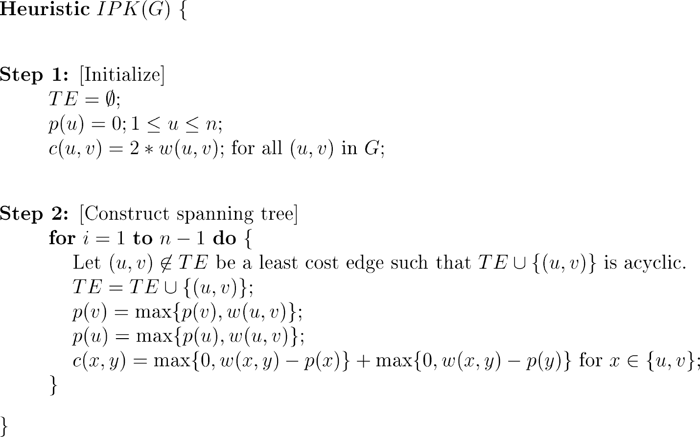
Figures 2 and 3 specify the IPK and IPP heuristics. Let p(TE) be the sum of the p(u)s. For edges eligible for selection in each iteration of the for loop, c(u, v) gives the incremental cost of adding (u, v) to TE. All references to cost in these heuristics are to c(∗, ∗). It is easy to see that following each iteration of the for loop, p(u) = max {w(u, v)|(u, v) ∊ TE}. The resemblance to Kruskal's and Prim's minimum cost spanning tree algorithms is evident.

Figure 2.

IPK heuristic for MPSC.

Figure 3.

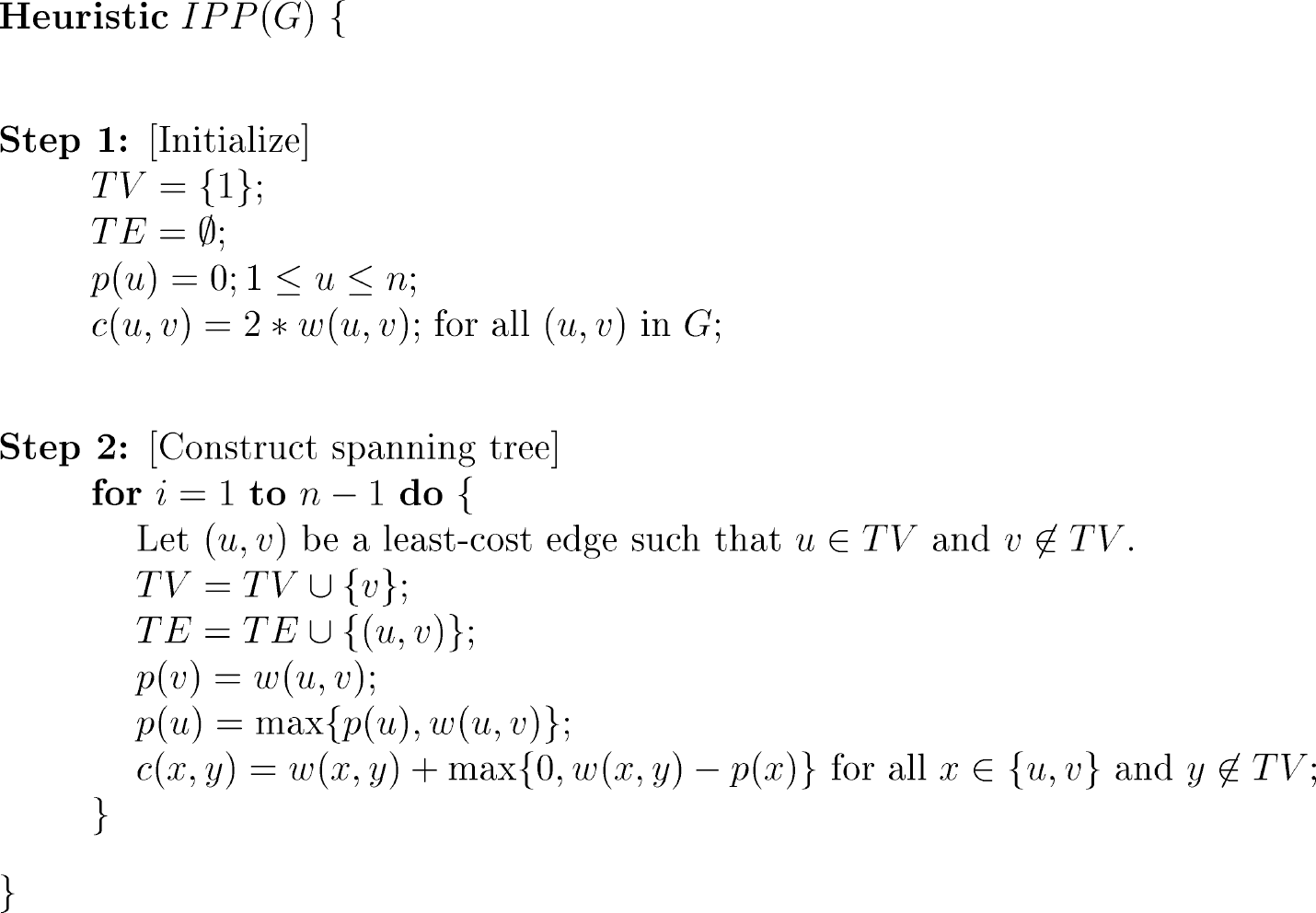
IPP heuristic for MPSC.

Figure 4 shows an example for IPP. Figure 4(a) shows the sensor network with edge weights equal to the transmission power needed. The number outside a vertex is its current p() value. The weight for each missing edge is ∞. Figure 4(b) shows the initial edge costs (twice the edge weights) and the initial TV (shaded vertex). This is the configuration at the start of the first iteration of the for loop. Each G_i, i < 8 gives the edge costs, p(), TV (shaded vertices) and TE (solid edges) at the start of the ith iteration of the for loop. G₈ gives the final values.

Figure 4.

Example for IPP.

Theorem 1. IPK and IPP have approximation ratio 2 for MPSC

Proof. Consider either IPK or IPP (the proof is identical for both). Let G_i be an undirected complete n-vertex graph in which the edge costs are the c(∗, ∗) values at the start of the ith iteration of the for loop. Let G_n be this graph at the end of the last iteration of the for loop, and let TE_i be TE at the start of the ith iteration of the for loop. Note that G₁ has c(u, v) = 2∗w(u, v), where w(u, v) is the power needed to transmit from u to v (equivalently, from v to u) and TE₁ = Ø. Let c(G_i) be the cost of the minimum cost spanning tree for G_i subject to the constraint that the spanning tree contain all edges in TE_i. In computing c(G_i), the cost of an edge (u, v) ∊ TE_i is its cost at the time it was selected for inclusion in TE and the cost of an edge (u, v) ∉ TE_i is its current c(u, v) value. Note that c(G_n) is the sum of p(∗) values when the heuristic terminates. This is so as, TE_n is a spanning tree and the sum of edge costs, where the cost of an edge is its c(∗, ∗) value at the time it was added to TE is the sum of the incremental power costs, which is the sum of the final p(∗) values.

From the correctness proof of Kruskal's and Prim's algorithms (see [12], for example), it follows that the edge selected for inclusion in TE in iteration i of the for loop is in the (constrained) minimum spanning tree of G_i. This together with the observation that the cost of the edges eligible for selection in the remaining iterations is no more in G_i+1 than in G_i implies that c(G_i+1) ≤ c(G_i). Hence, c(G_n) ≤ c(G₁).

Note that c(G₁) = 2w(MST), where MST is the minimum cost spanning tree for G₁ and w(MST) is the sum of weights (w(∗, ∗), not c(∗, ∗) values) of the edges in MST. In [3, 19, 10], it is shown that w(MST) < p(OPT), where OPT is an optimal power assignment and p(OPT) is the sum of the power levels in OPT. So, we have

c (G_{n}) \leq c (G_{1}) = 2 w (M S T) < 2 p (O P T)

Since c(G_n) is the sum of the power levels when the heuristic terminates, the heuristic has approximation ratio 2.

Theorem 2. The bound of Theorem 1 is tight

Proof. Figure 5(a) shows a sensor network. The edges show the permissible one-hop transmissions together with the required transmission power. Note that the weight assignments do not correspond to ideal E² distances. As noted in Section 1, the ideal situation almost never arises in practice because of media heterogeneity. Using the symmetric communication graph (which is a spanning tree of Fig. 5(a)) of Fig. 5(b) results in an optimal power assignment. In this power assignment, the power level of each node on the top row is set to ∊ and that for each node on the bottom row is set to 1. If the total number of nodes is 2n (n in each row of nodes), the cost of the optimal power assignment is n(1 + ∊). Using a suitable tie breaker, both IPK and IPP construct the spanning tree shown in Fig. 5(c). This spanning tree corresponds to a power assignment of ∊ to each node on the lower row; the assignment for the top row (left to right) is 1, 1.5 − ∊/2, 1.75 − 3∊/4, 1.875 − 7∊/8, …. The cost of this power assignment is

\begin{aligned} 1 + (n - 1) (2 - \in) - (1 - \in) \sum_{i = 1}^{n - 1} 1 / 2^{i} - (1 - \in) / 2^{n - 1} \\ = 2 n - 1 + \in - (1 - \in) [1 / 2^{n - 1} + \sum_{i = 1}^{n - 1} 1 / 2^{i}] \end{aligned}

Figure 5.

Example for Theorem 2.

As n gets large, the ratio of the cost of the IPK and IPP power assignment to the optimal one approaches 2/(1 + ∊), which approaches 2 as ∊ becomes small.

Theorem 3. Let p(IPK) and p(IPP), respectively, be the sum of the power assignments obtained by IPK and IPP. Let p(MST) be this quantity for the minimum cost spanning tree. 0.5 ≤ p(X)/p(MST) ≤ 2 for X ∊ {IPK, IPP}. Also, these bounds are tight

Proof. [3, 4, 10] show that p(MST) ≤ 2p(OPT), where OPT is the optimal power assignment. From this and Theorem 1, it follows that

\begin{aligned} p (O P T) & \leq p (M S T) \leq 2 p (O P T) \\ p (O P T) & \leq p (X) \leq 2 p (O P T) \end{aligned}

So, 0.5 ≤ p(X)/p(MST) ≤ 2.

To see that these bounds are tight, consider the sensor network of Fig. 5(a). Using a suitable tie breaker, the minimum cost spanning tree produced by Kruskal's and Prim's algorithm is that shown in Fig. 6(a). It's power cost is n(1 + ∊) + 1 − ∊, where n is the number of vertices in the top row. The spanning tree generated by X is shown in Fig. 5(c). Its power cost approaches 2(n + 1) − 2 as n → ∞. So, as n gets large, p(X)/p(MST) approaches 2.

Figure 6.

Example for Theorem 3.

Now consider the network of Fig. 6(b). Figure 6(c) shows a possible minimum cost spanning tree obtained by Kruskal's and Prim's algorithm. This results in assigning a power level of 2 to all vertices except 2. So, p(MST) is 4n − 4 + 2∊. Heuristic X, with a suitable tie breaker, produces the spanning tree shown in Fig. 6(d). This results in a power assignment of ∊ to each top-row vertex and 2 to each bottom-row vertex. So, p(X) = n(2 + ∊). By choosing n and ∊ appropriately, p(X)/p(MST) can be made as close to 0.5 as desired.

4. Enhancements

In this section, we describe three strategies to reduce the cost p(T) of the spanning tree T. Although these strategies do not reduce the approximation ratio of the MST, IPK, and IPP heuristics, they result in spanning trees that have lower p(T) value on average.

4.1. Sweep Method

Performing a sweep to improve the quality of a spanning tree has been done in the past in the context of the MEBT problem [15, 16, 11]. We propose an adaptation of this method to the MPSC problem. The sweep method of [15, 16, 11] is not directly applicable to MPSC because in MEBT we are dealing with asymmetric communication while in MPSC, we have symmetric communication. In a sweep, we start by selecting a vertex v of the spanning tree T as the tree root. Following this selection, child-parent relationships are uniquely determined. We perform a level-order traversal [12] of T beginning at the root v. When a node u is visited during this traversal, we perform the steps shown in Fig. 7.

Figure 7.

Visiting a node u during a sweep.

As an example, consider the tree T of Fig. 8(a). Let u be the root, A, of this tree. Suppose that p(A) ≥ w(A, D). So, D is selected as vertex v in Step 1. To get T^′ we move D together with its subtrees so that D becomes a child of A. This gives us T^′ as shown in Fig. 8(b). When the power levels are adjusted as in Steps 4 and 5, symmetric communication using T^′ is possible. If p(T^′) < p(T), we continue with T^′ as the working tree. Otherwise, we continue with T. Regardless, during the current visit, D cannot again be selected as the v vertex in Step 1. For an n-vertex spanning tree, the complexity of the visit operation is O(n). In a sweep, each vertex is visited once. So, the complexity of a sweep is O(n²).

Figure 8.

The sweep method.

4.2. Single Edge Switch (ES1a and ES1b)

Figures 9 and 10 give the edge switching heuristics ES1a and ES1b. In heuristic ES1a, the edge f is an edge on the unique cycle in T ∪ (u, v). In particular, f may be (w, v). To determine the power of T − {f} we need to first adjust the power level of the nodes u, v and the end points of f so that these nodes have the minimum power needed to do a single-hop transmission to their tree neighbors. Note that since (u, v) is a candidate for f, the minimum power of T − {f} is no more than that of the tree at the start of the for loop iteration. In ES1b, f is an edge that joins the two connected components of T − {(u, v)}. In particular, f could be (u, v). Once again to compute the power of T ∪ {f}, the power level of the nodes u, v and the end points of f need to be adjusted as in the case of ES1a.

Figure 9.

Heuristic ES1a.

Figure 10.

Heuristic ES1b.

Figure 11 shows an example for one iteration of the for loop of ES1a. Figure 11(a) shows the tree T at the start of the iteration. The numbers outside a node (e.g., (58) outside v1) give the power level of the node. The power cost of this tree is 336. Numbers outside edges are edge weights. (u, v) = (v4, v7) is added to T. This results in the cycle v4, v7, v1, v6, v4. The choices for f are (v4, v7), (v7, v1), (v1, v6) and (v6, v4). f = (v1, v7) results in p(v1) reducing from 58 to 10 and p(v7) increasing from 58 to 74. The remaining power levels are unchanged. The net reduction in tree power is 32. No other choice of f gives a larger reduction. So, we choose f = (v1, v7) and the new T is as shown in Fig. 11(c). This completes one iteration of the for loop. In this iteration, p(T) was reduced from 336 to 304.

Figure 11.

One iteration of the for loop of ES1a.

Figure 12 shows a single iteration of the for loop of ES1b. (u, v) = (v1, v7) ∊ T for this iteration. The edge f that reconnects T − {(u, v)} and results in minimum total power is (v4, v7). The result of switching edges (v1, v7) and (v4, v7) is a reduction of 32 in tree power.

Figure 12.

One iteration of the for loop of ES1b.

ES1b, which is the edge switching heuristic of [20], is simpler than the ES heuristic of [17]. Let (e₁, e₂), be a pair of edges such that e₁ is in the tree and e₂ is not. This edge pair defines a legal swap iff deleting e₁ from the tree and adding e₂ results in a spanning tree. In each iteration of ES, an edge pair that defines a legal swap that results in a min power cost spanning tree is determined. If the edge swap reduces the power cost, the swap is made and we proceed to the next iteration. Otherwise, the algorithm terminates.

Let e be the total number of edges. The complexity of both ES1a and ES1b is O(n²e).

Theorem 4. The approximation ratios of IPK and IPP remain 2 when these heuristics are enhanced by either or both of the methods sweep and single edge switch

Proof. follows from Theorem 2 and the observation that neither of the stated methods is able to reduce the power cost when started with the IPK and IPP spanning tree of Fig. 5(c).

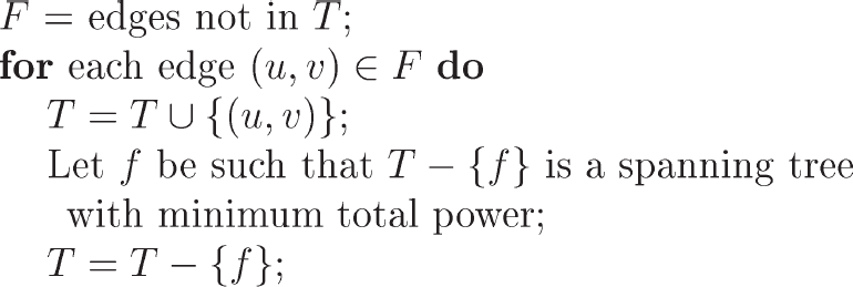
4.3. Double Edge Switch (ES2)

Double edge switching is like ES. However, in each iteration we find 4 edges e₁, e₂, e₃, e₄) such that the first 2 are in the tree and the last 2 are not. The 4 edges define a legal swap iff replacing the first two by the last two results in a spanning tree. As before, a legal swap that results in the minimum power cost spanning tree is determined. The swap is done iff it results in a power reduction. The process continues until no further reduction in power cost is obtainable by a legal swap. We note that ES2 generalizes the two-edge switching used in the EFS heuristic of [17]. In EFS, the edges e₃ and e₄ are required to form a fork (i.e., the two edges must share a vertex). The complexity of ES2 is O(n³e²).

5. Experimental Results

The MST, IPK, and IPP heuristics together with their enhancements were programmed in C++ and their relative performance compared using random graphs. MST was used as the benchmark heuristic for comparison purposes. Our random graphs were generated in a manner similar to that used in [17] to generate test graphs. We experimented with networks that have n ∊ {10, 50, 100} nodes. For each n, we generated 50 random graphs. Each random graph was generated by randomly assigning the n nodes to points in a 10000 × 10000 grid. We computed w(i, j) = r(i, j)^d, where r(i, j) is the Euclidean distance between nodes i and j, and d was set to 2.

Figure 13(a) gives the average percent reduction in power cost realized using either IPK or IPP over the power cost resulting from MST. This average reduction in power cost is between 2% and 3%. Also, IPP results in better power assignments than obtained by IPK.

Figure 13.

Average percent improvement over MST.

Figure 13(b) gives the average percent reduction in power cost realized by the sweep enhancement of MST (MST_SW), IPK (IPK_SW), and IPP (IPP_SW) over the power cost resulting from MST and Figs. 13(c)–(e), respectively, do this for the ES1a, ES1b, and ES2 enhancements of MST, IPK and IPP. Figures 15 and 16 give this average power-cost reduction data together with the minimum and maximum power-cost reductions and the standard deviations for the cases n = 50 and 100, respectively. Figure 14 shows the average power cost of the generated power assignments. This figure has separate bar charts for each of MST, IPK, and IPP together with their enhancements.

Figure 14.

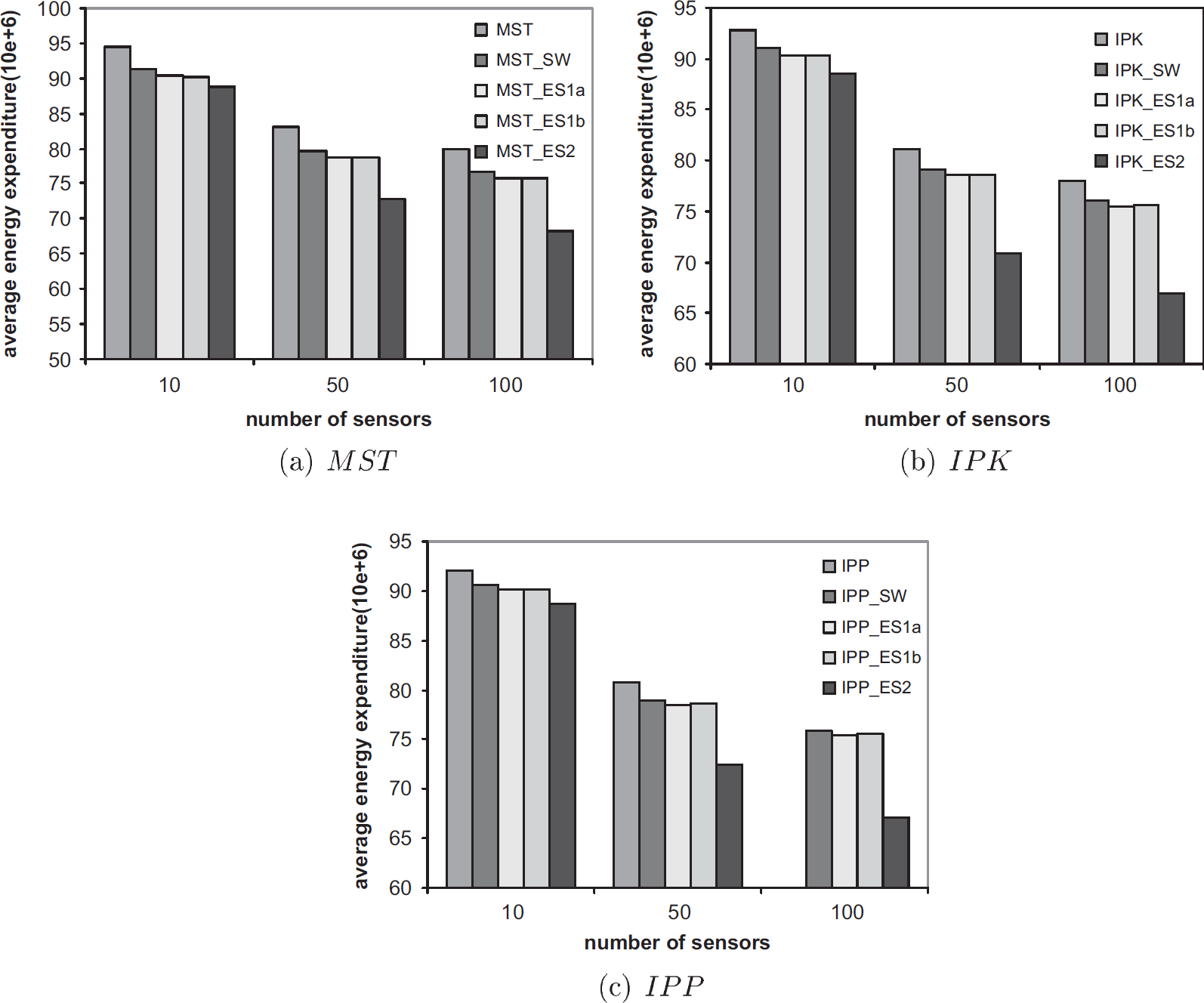
Average power cost.

Figure 15.

Percent power-cost reduction over MST for n = 50.

Figure 16.

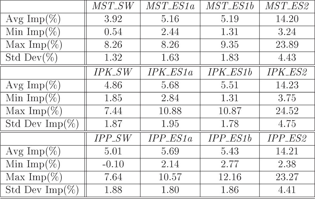
Percent power-cost reduction over MST for n = 100.

As can be seen from the provided data, the sweep enhancements of MST, IPK, and IPP, on average, result in a reduction in power cost between 3.9% and 5% relative to the power cost from MST. The ES1a and ES1b enhancements are about equally effective and both are superior to the sweep enhancement. These enhancements improve upon the MST power cost by between 5.2% and 5.7%. However, the greatest power-cost reductions relative to MST come when ES2 is employed. Now, the average reduction ranges from 12.5% to 14.2%. The maximum reduction observed on our test data was 24.5%. Note that since the approximation ratio for MST is 2, a reduction more than 50% is not possible.

Our experimental results are consistent with those reported in [17]; single-edge switch reduces the power-cost of MST by between 5% and 6%. Although the best heuristics of [17] are able to improve upon MST by at most about 6.5% (on average), our ES2 enhancement provides an improvement that is twice as much. Also, with the ES2 enhancement, IPK generally did better than MST and IPP.

6. Conclusion

We have shown that the approximation ratio for both IPP and IPK is 2. Further, none of the enhancements-sweep, ES1a, ES1b, ES2-reduce this approximation ratio. Our experiments show that the ES2 enhancement, on average, yields a power-cost reduction (relative to MST) by about twice as much as obtained by the best heuristics proposed in [17].

Footnotes

1

When a directed graph contains the directed edges (u, v) and (v, u), we say that (u, v) is bidirectional. A bidirectional edge may be modeled as an undirected edge. Hence, we use the terms bidirectional and undirected interchangeably.

References

Das

A. K.

Marks

R. J.

El-Sharkawi

, “Minimum power broad-cast trees for wireless networks,” IEEE International Symposium on Circuits and Systems, May 2002.

Egecioglu

Gonzalez

, “Minimum-energy broadcast in simple graph with limited node power,” IASTED International Conference on Parallel and Distributed Computing and Systems vol. 30, no. 4, pp. 334–338, August 2001.

Chen

Huang

, “The strongly connecting problem on multihop packet radio networks,” IEEE Trans. on Comm. 3, 293–295, 1989.

Cheng

Narahari

Simha

Cheng

Liu

, “Strong minimum energy topology in wireless sensor networks: NP-completeness and heuristics,” IEEE Trans. on Mobile Computing vol. 2, no. 3, 2003, pp. 248–256.

Chu

Nikolaidas

, “Energy efficient broadcast in mobile ad hoc networks,” AD-Hoc Networks and Wireless, 2002.

Clementi

Crescenzi

Penna

Rossi

Vocca

, “On the complexity of computing minimum energy consumption broadcast subgraphs.” Symp. on Theo. Aspects of Comp. Sci., 2001, pp. 121–131.

Clementi

Penna

Silvestri

, “On the power assignment problem in radio networks,” Electronic Colloquium on Computational Complexity 054, 2000.

Garey

Johnson

, Computers and Intractability: A Guide to the Theory of NP-completeness. W. H. Freeman and Co., 1979.

Guha

Khuller

, “Approximation algorithms for connected dominating sets,” Fourth Annual European Symposium on Algorithms, 1996.

10.

Kirousis

Kranakis

Krizanc

Pelc

, “Power consumption in packet radio networks.” Theo. Comp. Sci. 243, pp. 289–305,2000.

11.

Park

Sahni

, “Maximum lifetime broadcasting in wireless networks,” IEEE Trans. on Computers, 2005.

12.

Sahni

, Data Structures, Algorithms, and Applications in Java. 2nd Edition, Silicon Press, NJ, 2005.

13.

Singh

Raghavendra

Stepanek

, “Power-aware broadcasting in mobile ad hoc networks,” IEEE PIMRC′99, Sep. 1999, Japan.

14.

Wan

Calinescu

Frieder

, “Minimum energy broadcast routing in static ad hoc wireless networks,” IEEE INFOCOM, 2001.

15.

Wieselthier

Nguyen

Ephremides

, “On the construction of energy-efficient broadcasting and multicast trees in wireless networks,” IEEE INFOCOM, 2000.

16.

Wieselthier

Nguyen

, “Algorithm for energy-efficient multicasting in static ad hoc wireless networks,” Mobile Networks and Applications, 2001, pp. 251–261.

17.

Althaus

Calinesu

Mandoiu

I.I.

Prasad

Tchervenski

Zelikovsky

, “Power efficient range assignment in ad-hoc wireless networks,” In Proceedings of IEEE Wireless Communications and Networking Conference (WCNC′03), pp. 1889–1894, 2003.

18.

Bolugh

D.M.

Leoncini

Resta

Santi

, “On symmetric range assignment problem in wireless ad hoc networks,” TCS 2002, pp. 71–82, 2002.

19.

Calinescu

Mandoiu

I.I.

Zelikovsky

A.Z.

, “Symmetric connectivity with minimum power consumption in radio networks,” TCS 2002, pp. 119–130, 2002.

20.

Calinescu

Mandoiu

I.I.

Zelikovsky

A.Z.

, Powerpoint presentation. “Symmetric connectivity with minimum power consumption in radio networks,” TCS 2002, pp. 119–130, 2002.

21.

Ramanathan

Rosales

, “Topology control of multihop wireless networks using transmit power adjustment,” IEEE INFOCOM, 2000.

22.

Rappaport

, Wireless Communications: Principles and Practices Prentice Hall, 1996.

23.

Cheng

Narahari

Simha

Liu

, “Strong minimum energy topology in wireless sensor networks: NP-completeness and heuristics,” IEEE Transactions on Mobile Computing vol. 2, no. 3, pp. 248–256, 2003.