Sage Journals: Discover world-class research

Abstract

Data aggregation promises a new paradigm for gathering data via collaboration among wireless sensors deployed over a large geographical region. Many real-time applications impose stringent delay requirements and ask for time-efficient schedules of data gathering in which data sensed at sensors are aggregated at intermediate sensors along the way towards the data sink. The Minimal Aggregation Time (MAT) problem is to find the schedule that routes data appropriately and has the shortest time for all requested data to be aggregated and sent to the data sink.

In this article we consider the MAT problem with collision-free transmission where a sensor can not receive any data if more than one sensors within its transmission range send data at the same time. We first prove that the MAT problem is NP-hard even if all sensors are deployed on a grid. We then propose a (Δ −1)-approximation algorithms for the MAT problem, where Δ is the maximum number of sensors within the transmission range of any sensor. By exploiting the geometric nature of wireless sensor networks, we obtain some better theoretical results for some special cases. We also simulate the proposed algorithm. The numerical results show that our algorithm has much better performance in practice than the theoretically proved guarantees and outperforms other existing algorithms.

Keywords

Wireless Sensor Networks Data Aggregations Convergecast Collision-free Transmission Unit Disk Graphs Approximation Algorithm

1. Introduction

Due to various existing and potential applications, Wireless Sensor Networks (WSNs) have recently emerged as a premier research topic. A WSN usually consists of a large number of small-sized and low-powered sensors deployed over a geographical area and a sink node where the end user can access data. All nodes are equipped with capabilities of sensing, data processing, and communicating with each other by means of a wireless ad hoc network. A wide range of tasks can be performed by these tiny devices, such as condition-based maintenance and the monitoring of a large area with respect to some given physical quantity, e.g., temperature, humidity, gravity, and seismic information.

In contrast to traditional networks (e.g., the Internet) which are address-centric, WSNs are intrinsically data-centric. In some applications of WSN, the end user needs to extract information from the sensor field with low latency. In this case, data sensed at some sensors related to the same physical phenomenon need to be aggregated and sent to the data sink efficiently. Real time data aggregation is a combination of data from different sensors according to a certain aggregation function, e.g., duplicate suppression, logical AND/OR, minima and maxima, and all requested data should be periodically delivered to the sink node within a certain period of time from the moment they are requested (after that data may be useless).

The stringent resource constraint and the sheer number of sensor nodes in WSNs pose unique challenges on time-efficient data aggregation. First, the sensor nodes operate on batteries and employ low-power radio transceivers to enable communications. Data packet sent by a senor (sender) reaches all its neighbor nodes within the transmission range of the sender; Sensors far from the data sink have to use intermediate nodes to relay data transmission. Second, collision resulting from a large number of simultaneous sending creates response implosion [1]: when two or more sensors send data to a common neighbor at the same time, collision occurs at this node, which will not receive any of these data.

Third, the data sent by a sender is received by any its neighbor (receiver) at which no collision occurs; the receiver fuses the data received with its own data (possibly null), and stores the fused data as its new data. In addition, the time consumed by a single sending-receiving-fusing-storing is typically normalized to one; parallel sending-receiving are desirable for reducing the network delay. Fourth, with the large population of sensor nodes, it may be impractical or energy consuming to pay attention to each individual node in all situations; for instance, the user wound be more interested in querying “what is the highest temperature in some specified areas?”

Motivated by various applications of time-efficient data aggregation for query-based monitoring WSNs, we study in this paper the Minimum Aggregation Time (MAT) Problem under collision-free transmission model, which guarantees the energy-efficiency since no data need to be transmitted more than once. The problem is how to, given a WSN with a distinguished data sink d which is interested in data on a subset S of sensor nodes, determine a data transmission schedule such that all data on S are sent and aggregated to d in the minimum time.

The remainder of the article is organized as follows. In Section 2, we first specify the network model and formalize the MAT problem, and then present some related works and summarize our contributions in this paper. In Section 3, we prove that the MAT problem is NP-hard even for some special case. In Section 4, we propose some approximation algorithms for the MAT problem, and give the theoretical proofs of their performance guarantees. In Section 5, we evaluate the average performance of the proposed algorithm through simulation and compare it with the existing algorithm. In Section 6, we conclude the article discussing on how to implement the proposed algorithm to achieve energy-efficiency as well as time-efficiency.

2. Preliminaries

2.1. Model Description

In view of the miniature design of sensor devices, we assume that all sensors in WSNs are fixed and homogeneous. More specifically, the WSN under investigation consists of stationary nodes (sensor nodes and a sink node) distributed in a Euclidean plane. Assuming the transmission range of any sensor node is a unit disk (circular region with unit radius) centered at the sensor, we model a WSN as a unit disk graph (UDG) G = (V, E) in which two nodes u,v ∈ V are considered neighbors, i.e., there is an edge uv ∈ E joining u and ϛ, if and only if the Euclidean distance ‖ u− v‖ between u and ϛ is at most one. Hereafter we reserve symbol G for UDGs modelling WSNs, and Δ for the maximum degree of G. It is always assumed that G is connected. We assume in this paper that communication is deterministic and proceeds in synchronous rounds controlled by a global clock. In each time round,

Each node can send data (be a sender) or receive data (be a receiver) but cannot do both;

Each node can receive data from at most one of its neighbors;

Data packet sent by any sender reaches all its neighbors simultaneously;

Any node can receive data only if exactly one of its neighbors sends data.

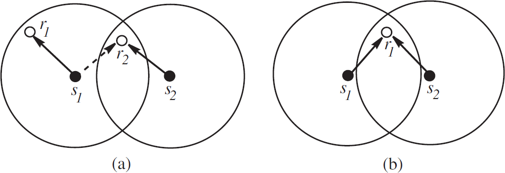
Note that the above conditions guarantee collision-free data transmit/receiving between senders and receivers. In Fig. 1a, two time rounds are required if s_i needs to send its data to r_i for i = 1, 2 since when they send their data in the same time round r₂ will receive data from both s₁ and s₂ causing collision, which is not allowed (due to Conditions (3–4)). For the same reason, in Fig. 1b, two time rounds are required if s₁ and s₂ both need to send their data to r₁. Moreover, we assume that each receiver updates its data as the combination of all data received in different rounds; this enforces that each node needs to send data at most once.

Figure 1.

Description of network assumptions.

An instance of the MAT problem is denoted by (G, S, d), where the set $S \subset V (G)$ consists of nodes whose data are requested by the sink node $d \in V$ . The solution of (G, S, d) is a schedule {(S₁, R₁), …, (S_s, R_s)} such that S_r (resp. R_r) is the set of senders (resp. receivers) in the r-th round for r = 1, 2, …, s, and all data on S must be aggregated to d within s rounds. Note that every (S_r, R_r) gives implicitly the 1-1 correspondence between S_r and R_r in a way that ϛ ∈ S_r corresponds to its receiver in R_r which is the only neighbor of ϛ in R_r. The value s is called the data aggregation time of solution {(S₁, R₁), …, (S_s, R_s)}. MAT problem is to find the schedule with minimum data aggregation time t_OPT(G, S, d).

As usual (e.g., in [2]), we assume that each sensor node knows its geometric position in the network, which is considered the unique ID of the sensor (the aggregated data may include some of these IDs). We further assume that the sink has global knowledge of IDs of all sensors in the WSN. When it needs some data of particular interests at some sensor nodes, it informs those nodes, by multicasting, of the schedule {(S₁, R₁), …, (S_s, R_s)} which may be represented by IDs of senders and receivers. Upon receiving the request, sensor nodes will send their data or receive data from others as specified in the schedule. In such a way, the schedule guarantees collision-free data aggregation. It also enables significant energy savings since sensor nodes are in an energy conserving state when they do not participate in sending/receiving. Prior to the scheduled time for data aggregation, a node switched from the energy conserving state to the energy consuming state, transmits or receives data and then goes back to the energy conserving state.

2.2. Related Works

Most of the works on data aggregation focus on energy efficiency such as [3], [4]. There are two recent works on time efficiency [5], [6]. They studied a special case of MAT problem, called convergecasting problem, where S = V\d (i.e., data at all sensors are required to be sent and aggregated to the data sink). Annamalai et al. [5] proposed a centralized heuristic that constructs a tree rooted at the sink node according to the proximity criterion (a node is assigned as a child to the closest possible parent node) and to assign each node a code and a time slot to communicate with its parent node. However, the miniature hardware design of nodes in WSNs may not permit employing complex radio transceivers required for spread spectrum codes or frequency bands systems. Additionally, the heuristic is evaluated only through simulations and no theoretical analysis for their methods was given. More recently, Kesselman and Kowalski [6] devised a randomized distributed algorithm for convergecasting that has the expected running time O(log|V|). An assumption central to their model is that sensor nodes have the capability of detecting collisions and adjusting transmission ranges, and that the maximum transmission range might be as large as the diameter of the network. This complicates the sensor hardware design and poses challenge to low-transmission-range constraint on sensors.

Minimum Broadcast Time (MBT) problem [7] is very similar to the MAT problem. Initially, d has a message to be broadcasted to every node in the network; At each time round any node that has received the message is allowed to communicate the message to at most one of its neighbors. MBT problem asks for the broadcast schedule of minimum number of time rounds required for every node receiving the message. This problem can be considered as a relaxed version of MAT problem with S = V\d which allows, in Fig. 1a, s₁ and s₂ to send their data to r₁ and r₂ at the same time round, respectively. Clearly, MBT problem schedules the data to flow from d to all nodes in S while MAT problem schedules data to flow from all nodes towards d. It is known that MBT problem is NP-hard [7] and has a 2Δ-approximation algorithm [8].

Given an MAT instance (G, S, d), a shortest path tree (SPT) T of (G, S, d) is a tree in G consisting of shortest paths from d to nodes in S. The height of T, denoted by h(G, S, d), equals to the length of the longest path in T from d to leaves of T. The following lower bound can be easily obtained by applying the same argument used in the estimation of multicasting time in telephone networks [9].

Lemma 2.1

t_OPT(G, S, d) ≥ max{h(G, S, d), log₂ |S|} for any MAT instance (G, S, d). However, data aggregation in WSNs is not simply the reverse of broadcast/multicast in traditional telephone network. For example, it was shown in [10] that the broadcast time in a WSN is at most 648 times the height of SPT. Note also when the underlying topology G of WSNs is a complete graph, we have t_OPT(G, S, d) = |V| while SPT gives a multicast time equal to 1 and MBT problem has minimum broadcast time of log₂|V|.

2.3. Our Contributions

The first contribution of our work is a new and simple data aggregation model. It is collision-free and does not require any specialized codes so that data aggregation can be conducted in an energy-conserving manner. The second contribution is the NP-hardness proof of the corresponding problem even when all nodes are deployed at integer coordinates in the Euclidean plane. The third contribution is an approximation algorithm proposed for the MAT problem with theoretically proved performance guarantees. The algorithm uses a new technique that allows certain flexibility of tree-structures while scheduling parallel transmissions; in other words, instead of making a schedule after a tree is constructed as the existing methods do, it forms a data aggregation tree after a schedule is made.

3. Complexity Analysis

In order to prove the NP-hardness of MAT problem, we will apply some known results on orthogonal planar drawing. An orthogonal planar drawing of a planar graph H is a planar embedding of H in the plane such that all edges are drawn as sequences of horizontal and vertical segments. A point where the drawing of an edge changes its direction is called a bend of this edge. All vertices and bends are drawn on integer points. If the drawing can be enclosed by a box of width g and height g, we call it an embedding with grid size g X g. By a plane graph we mean a planar graph together with a planar embedding of it. Biedl and Kant [11] proved the following lemma.

Lemma 3.1

Given a simple plane graph H on g vertices that is not an octahedron and has maximum degree at most 4, there is a linear algorithm which produces an orthogonal planar drawing of H with grid size g × g such that the number of bends along each edge is at most 2.

Using the above lemma we can deduce the following lemma whose proof is very sophisticated and thus given in the appendix at the end of the paper.

Lemma 3.2

Let H be a plane graph on g vertices with maximum degree at most 4. Suppose that H is not an octahedron, and let H' be the graph obtained from H by replacing each edge in H with a path of length 120g². Then H' is a unit disk graph and an orthogonal planar embedding of H' of grid size (40g² + 40g) × (40g² + 40g) can be computed in time polynomial in g.

We now explain how to prove that MAT problem is NP-hard by reducing the restricted planar 3-SAT problem to it. Let {x₁, …, x_n} and {c₁, …, c_m} denote, respectively, the sets of variables and clause in a Boolean formula Φ in conjunctive normal form, where each clause has at most 3 literals. Associate with Φ the formula graph $G_{φ} = ({x_{1}, \dots, x_{n}} \cup {c_{1}, \dots, c_{m}}, E_{1} \cup E_{2})$ , where $E_{1} := {x_{i} c_{j} : x_{i} \in c_{j} or {\bar{x}}_{i} \in c_{j}}$ and $E_{2} := {x_{i} x_{i + 1} : 1 \leq i \leq n - 1} \cup {x_{n} x_{1}}$ . The Boolean formula is called planar if G_Φ is a planar graph. The planar 3-SAT problem is to decide if there is a truth assignment that satisfies all clauses in a planar Boolean formula, where each clause has at most three literals. A planar 3-SAT problem is said to be restricted if

each variable (unnegated or negated) appears at most three clauses,

both unnegated and negated forms of each variable appear; and

at every variable node in the planar embedding of G_Φ, the edges in E₂ that are incident with node x separate the edges in E₁ incident to x such that all edges representing a nonnegative appearance are incident to one side of x and all edges representing a negative appearance are incident to the other side. It is known that the restricted planar 3-SAT problem is NP-complete [12].

Theorem 3.1

The decision version of MAT problem is NP-complete even when the underlying topology is a subgraph of a grid.

Proof

The proof is based on a reduction from restricted planar 3-SAT. Given any restricted planar 3-SAT instance ϕ on n variable and m clauses, from its planar formula graph G_ϕ, we construct planar graphs G_k for positive integer k as follows.

To every variable x_i, 1 ≤ i ≤ n, we associate a rectangle X_i and two node-disjoint paths $Π_{i}, {\bar{Π}}_{i}$ such that

(i)
X_i has exactly 10k nodes among which equally spaced nodes $p_{i}, q_{i}, r_{i}, s_{i}, t_{i}, {\bar{s}}_{i}, \bar{r_{i}}, {\bar{q}}_{i}, {\bar{p}}_{i}, {\bar{t}}_{i}$ are located in cyclic order of X_i, and II _i (resp. ${\bar{Π}}_{i}$ ) has ends o_i and p_i (resp. ${\bar{o}}_{i}$ and ${\bar{p}}_{i}$ ) with $Π_{i} \cap X_{i} = {p_{i}}$ (resp. ${\bar{Π}}_{i} \cap X_{i} = {{\bar{p}}_{i}}$ ), and
(ii)
both II _i and ${\bar{Π}}_{i}$ are of length $(6 i - 5) k - 1$ . To every clause c_j, we associate a path C_j with ends b_j, c_j and of length k −1. All $X_{i} \cup Π_{i} \cup {\bar{Π}}_{i}$ 's and C_j's are pairwise node-disjoint. For every edge x_ic_j (resp. ${\bar{x}}_{i} c_{j}$ ) in G_ϕ, there is a path $Υ_{i j}$ in G_k such that P_ij has one end c_j and the other end in {r_i, s_i} (resp. ${{\bar{r}}_{i}, {\bar{s}}_{i}}$ ), and for all $1 \leq i, i^{'} \leq n, 1 \leq j, j^{'} \leq m$ , we have
(iii)
$P_{i, j} \cap (⋃_{h = 1}^{n} C_{h}) = {c_{j}}, P_{i j} \cap (⋃_{h = 1}^{n} (X_{i} \cup Π_{i} \cup {\bar{Π}}_{i}))$ consists of a node in ${r_{i}, s_{i}, {\bar{r}}_{i}, {\bar{s}}_{i}}$ ;
(iv)
$P_{i j} \cap P_{i^{'} j^{'}} \neq \emptyset$ if $P_{i j} = P_{i^{'} j^{'}}$ or $i \neq i^{'}$ and $P_{i j} \cap P_{i^{'} j^{'}} = {c_{j}} = {c_{j^{'}}}$ ; and
(v)
P_ij is of length (6 _i — 4)k when it has an end in ${r_{i}, {\bar{r}}_{i}}$ and of length (6 _i — 3)k when it has end in ${s_{i}, {\bar{s}}_{i}}$ . Finally we add n — 1 pairwise disjoint paths $Λ_{1}, \dots, Λ_{n - 1}$ such that
(vi)
$Λ_{h}$ has length k and $Λ_{h} \cup (⋃_{i, j} (X_{i} \cup Π_{i} \cup {\bar{Π}}_{i} \cup P_{i j})) = {t_{h}, t_{h + 1}}$ for $h = 1, \dots, h - 1$ . This completes the construction of $G_{k} := ⋃_{i, j} (X_{i} \cup Π_{i} \cup \bar{Π_{i}} \cup Λ_{i} \cup C_{j} \cup P_{i j})$ .

Let $G_{k}^{+}$ be obtained from G_k by adding 2 _n + m pendant edges such that the 2 _n + m degree-one nodes $o_{1}, {\bar{o}}_{1}, o_{2}, {\bar{o}}_{2}, \dots, o_{n}, {\bar{o}}_{n}, b_{1}, b_{2}, \dots, b_{m}$ in G_k have degree two in $G_{k}^{+}$ . Denote by g the number of nodes in $G_{1}^{+}$ and set $ℓ = 120 g^{2}$ . It is easy to see that g < 36n² + m and that $G_{ℓ}^{+}$ is obtained from $G_{l}^{+}$ by replacing each edge of $G_{1}^{+}$ with a path of length 120g². Since G_ϕ is a planar graph with a maximum degree of at least 3, so is G₁. Thus a planar embedding of G₁ might be computed in time polynomial in n + m [13]. By the construction, this planar embedding might be extended to be a planar embedding for $G_{1}^{+}$ in time polynomial in g and hence polynomial in n + m. Notice that $G_{1}^{+}$ is a plane graph other than octahedron and that the maximum degree of $G_{1}^{+}$ is at most 4. It follows from Lemma 3.2 that $G_{ℓ}^{+}$ is a unit disk graph, so is G_ϕ. Moreover from Lemma 3.2, we deduce that G_ϕ is a subgraph of a grid, and that both the size of G_ϕ and the construction time of G_ϕ are polynomial in n + m.

Next we show that the restricted planar 3-SAT instance ϕ is satisfiable if and only if the MAT problem on ( $G_{ℓ}, V (G_{ℓ}), t_{n}$ ) has a solution (schedule) which aggregates all data on $V (G_{ℓ})$ into the sink t_n within $(6 n - 1) ℓ$ rounds. To this end, let us first make some observations. For notational convenience, we set $Λ_{n} = \emptyset$ and use $X_{i}^{+}$ (resp. $X_{i}^{-}$ ) to denote the shortest path from p_i to s_i (resp. ${\bar{p}}_{i}$ to ${\bar{s}}_{i}$ ), i = 1, 2. …, n. Clearly, $X_{i}^{+} \cup X_{i}^{-} \subseteq X_{i}, X_{i}^{i} \cap X_{i}^{-} = \emptyset, {p_{i}, q_{i}, r_{i}, s_{i}} \subseteq X_{i}^{+}$ and ${{\bar{p}}_{i}, {\bar{q}}_{i}, {\bar{r}}_{i}, {\bar{s}}_{i}} \subseteq X_{i}^{-}$ for all $1 \leq i \leq n$ .
Every shortest path from ${\bar{t}}_{1}$ to t_n is of length $(6 n - 1) ℓ$ and must be contained in $⋃_{ι = 1}^{n} (X_{ι} \cup Λ_{ι})$ .

Suppose the contrary that P is a shortest path from ${\bar{t}}_{1}$ to t_n violating (a). Then by (i) and (vi), we have $P ⊈ ⋃_{ι = 1}^{n} (X_{ι} \cup Λ_{ι})$ . Then there exist $1 \leq h < i \leq n$ and $1 \leq j \leq m$ such that $P_{h j} \cup P_{i j}$ is a subpath of P. Let u_h (resp. u_i) denote the the end of P_hj (resp. P_ij) in X_h (resp. X_i). By symmetry suppose that the shortest path in X₁ from ${\bar{t}}_{1}$ to r₁ is a subpath of P. It is clear that $P ∖ ((P_{h j} \cup P_{i j}) ∖ {u_{h}, u_{i}})$ consists of two paths P₁ and P₂ with P₁ containing ${\bar{t}}_{1}, r_{1}, u_{h}$ and P₂ containing u_i, t_n. Note from (i), (v) and (vi) that $(\cup_{ι = 1}^{i - 1} (X_{ι} \cup Λ_{ι})) \cup X_{i}$ contains a path Q from r₁ to u_i of length $| E (Q) | = | E (p_{i j}) | - 2 ℓ$ . It is not hard to see that $P_{1} \cup Q \cup P_{2}$ contains a path P' from ${\bar{t}}_{1}$ to t_n shorter than P, a contradiction. So (a) holds. Combining (a) with (ii) and (v), we have

For $1 \leq i \leq n, (⋃_{ι = i}^{n} (R_{ι} \cup Λ_{ι})) ∖ {\bar{t}}_{i}$ contains every shortest path from o_i (resp. ${\bar{p}}_{i}$ ) to t_n (which is of length $(6 (n - i) + 4) ℓ)$ , every shortest path from r_i (resp. ${\bar{r}}_{i}$ ) to t_n (which is of length $(6 (n - i) + 2) ℓ)$ , and every shortest path from s_i (resp. ${\bar{s}}_{i}$ ) to t_n (which is of length $(6 (n - i) + 1) ℓ)$ .

For $1 \leq i \leq n$ , every shortest path from o_i (resp. ${\bar{o}}_{i}$ ) to t_n has length $(6 n - 1) ℓ - 1$ and its intersection with $⋃_{ι = 1}^{n} (X_{ι} \cup Λ_{ι})$ is a path from p_i (resp. ${\bar{p}}_{i}$ ) to t_n containing $X_{i}^{+}$ (resp. $X_{i}^{-}$ ) and avoiding $X_{i}^{-}$ (resp. $X_{i}^{+}$ ); and no path from o_i (resp. ${\bar{o}}_{i}$ ) to t_n has length $(6 n - 1) ℓ$ .

For $1 \leq j \leq m$ , each shortest path from b_j to t_n has length $(6 n - 1) ℓ - 1$ and its intersection with $⋃_{i = 1}^{n} (X_{i} \cup Λ_{i})$ is a path; and no path from b_j to t_n has length $(6 n - 1) ℓ$ .

Now we assume that all data on V( $G_{ℓ}$ ) are aggregated into t_n within $(6 n - 1) ℓ$ rounds. It is immediate from (a) that the data on ${\bar{t}}_{1}$ is aggregated up to t_n along a shortest path P from ${\bar{t}}_{1}$ to t_n in $⋃_{ι = 1}^{n} (R_{ι} \cup Λ_{ι})$ without any delay; particularly, we have
for $1 \leq i \leq n, | P \cap {X_{i}^{+}, X_{i}^{-}} | = 1$ .

For $i = 1, \dots, n$ let ${w_{i}, {\bar{w}}_{i}} = {p_{i}, {\bar{p}}_{i}}, {x_{i}, {\bar{x}}_{i}} = {q_{i}, {\bar{q}}_{i}}, {y_{i}, {\bar{y}}_{i}} = {r_{i}, {\bar{r}}_{i}}$ and ${z_{i}, {\bar{z}}_{i}} = {s_{i}, {\bar{s}}_{i}}$ be such that P contains w_i, x_i, y_i, z_i. Inductive arguments show that

for $1 \leq i \leq n$ , the aggregated data from ${\bar{t}}_{1}$ is received by ${\bar{t}}_{i}$ in round $(6 i - 6) ℓ$ , by w_i in round $(6 i - 5) ℓ$ , by y_i in round $(6 i - 3) ℓ$ , by z_i in round $(6 i - 2) ℓ$ , and by t_i in round $(6 i - 1) ℓ$ .

Note from (c) that the data on o_i (resp. ${\bar{o}}_{i}$ ) must be aggregated towards t_n along a shortest path from o_i (resp. ${\bar{o}}_{i}$ ) to t_n containing $Π_{i} \cup X_{i}^{+}$ (resp. $Π_{i} \cup X_{i}^{-}$ ), and o_i (resp. ${\bar{o}}_{i}$ ) sends data in round 1 or in round 2. Since by (i) and (ii) the length of $Π_{i} \cup X_{i}^{+}$ (resp. $Π_{i} \cup X_{i}^{-}$ ) is $(6 i - 2) ℓ - 1$ , we see that o_i (resp. ${\bar{o}}_{i}$ ) collide on w_i in round $(6 i - 5) ℓ$ or collide on t_i in round $(6 i - 1) ℓ$ . Let ϛ _i = o_i if $w_{i} = {\bar{p}}_{i}$ and $v_{i} = {\bar{o}}_{i}$ if w_i = p_i. Then
for $1 \leq i \leq n$ , the aggregated data from ϛ _i is received by ${\bar{w}}_{i}$ in round $(6 i - 5) ℓ - 1$ , by ${\bar{y}}_{i}$ in round $(6 i - 3) ℓ - 1$ , by ${\bar{z}}_{i}$ in round $(6 i - 2) ℓ - 1$ , and by t_i in round $(6 i - 1) ℓ - 1$ .

Let us consider an arbitrary $j \in {1, \dots, m}$ . It can be seen from (d) that the data on b_j is aggregated to t_n along a shortest path from b_j to t_n without any delay. Obviously this shortest path contains $C_{j} \cup P_{i j}$ as a subpath for some $i \in {1, \dots, n}$ . Recall from (v) that $C_{j} \cup P_{i j}$ is of length $(6 i - 3) ℓ - 1$ when one end of P_ij is in ${r_{i}, {\bar{r}}_{i}}$ , and of length $(6 i - 2) ℓ - 1$ when one end of P_ij is in ${s_{i}, {\bar{s}}_{i}}$ . If ${\bar{y}}_{i}$ is an end of P_ij, then data from ϛ _i and the data from b_j collide on ${\bar{y}}_{i}$ in round $(6 i - 3) ℓ - 1$ . So we have ${\bar{y}}_{i} \notin P_{i j}$ , and similarly ${\bar{z}}_{i} \notin P_{i j}$ . It follows that for every $1 \leq j \leq m$ , there exists some P_j on the aggregation path from b_j to t_n such that $P_{i j} \cap {y_{i}, z_{i}} \neq \emptyset$ . This allows us to derive a truth assignment for ϕ by setting $x_{i} := t r u e iff X_{i}^{+} \subseteq P$ .

Conversely, we consider the case where the restricted planar 3-SAT instance ϕ has a true assignment {x₁∗, x₂∗, x_n∗}. Notice that for each $1 \leq j \leq m$ , there exists some $j (i) \in {1, \dots, n}$ such that either $t r u e = x_{j (i)}^{} \in C_{j}$ and P_j(i)j* connects c_j with r_j(i) or s_j(i), or $t r u e = {\bar{x}}_{j (i)}^{} \in C_{j}$ and P_j(i)j* connects c_j with ${\bar{r}}_{j (i)}$ or ${\bar{s}}_{j (i)}$ . To define a schedule for the MAT problem on $(G_{ℓ}, V (G_{ℓ}), t_{n})$ , from $G_{ℓ}$ we construct a spanning T of $G_{ℓ}$ rooted at t_n by deleting some edges of $G_{ℓ}$ as follows: For each $1 \leq i \leq n$ , we delete the edge incident with ${\bar{t}}_{i}$ contained in $X_{i}^{-}$ (resp. $X_{i}^{+}$ ) when $x_{i}^{} = t r u e$ (resp. $x_{i}^{} = t r u e$ ); for each $1 \leq j \leq m$ , we delete all edges incident with c_j but the two in $C_{j} \cup P_{j (i) j}$ . From (i)-(vi) and (a)-(d), it is easy to see that the height of T is $(6 n - 1) ℓ$ . Now for $i = 1, 2, \dots, (6 n - 1) ℓ$ , let S_i consist of all nodes such that the paths in T from tn to them have length $(6 n - 1) ℓ - i + 1$ , and let R_i consist of parents (in T) of nodes in S_i. Again (i)-(vi) and (a)-(d) assure that ${(S_{1}, R_{1}), (S_{2}, R_{2}), \dots, (S_{(6 n - 1) ℓ}, R_{(6 n - 1) ℓ})}$ is a schedule with data aggregation time $(6 n - 1) ℓ$ for MAT problem on $(G_{ℓ}, V (G_{ℓ}), t_{n})$ . The theorem is proved.
4. Approximation Algorithms

In this section we present an approximation algorithms SDA for the MAT problem that adopts the shortest data aggregation strategy: aggregating data along the shortest paths towards the sink. Theoretical analysis provide the worst-case performance ratios of the algorithm.

4.1. Basic Algorithm

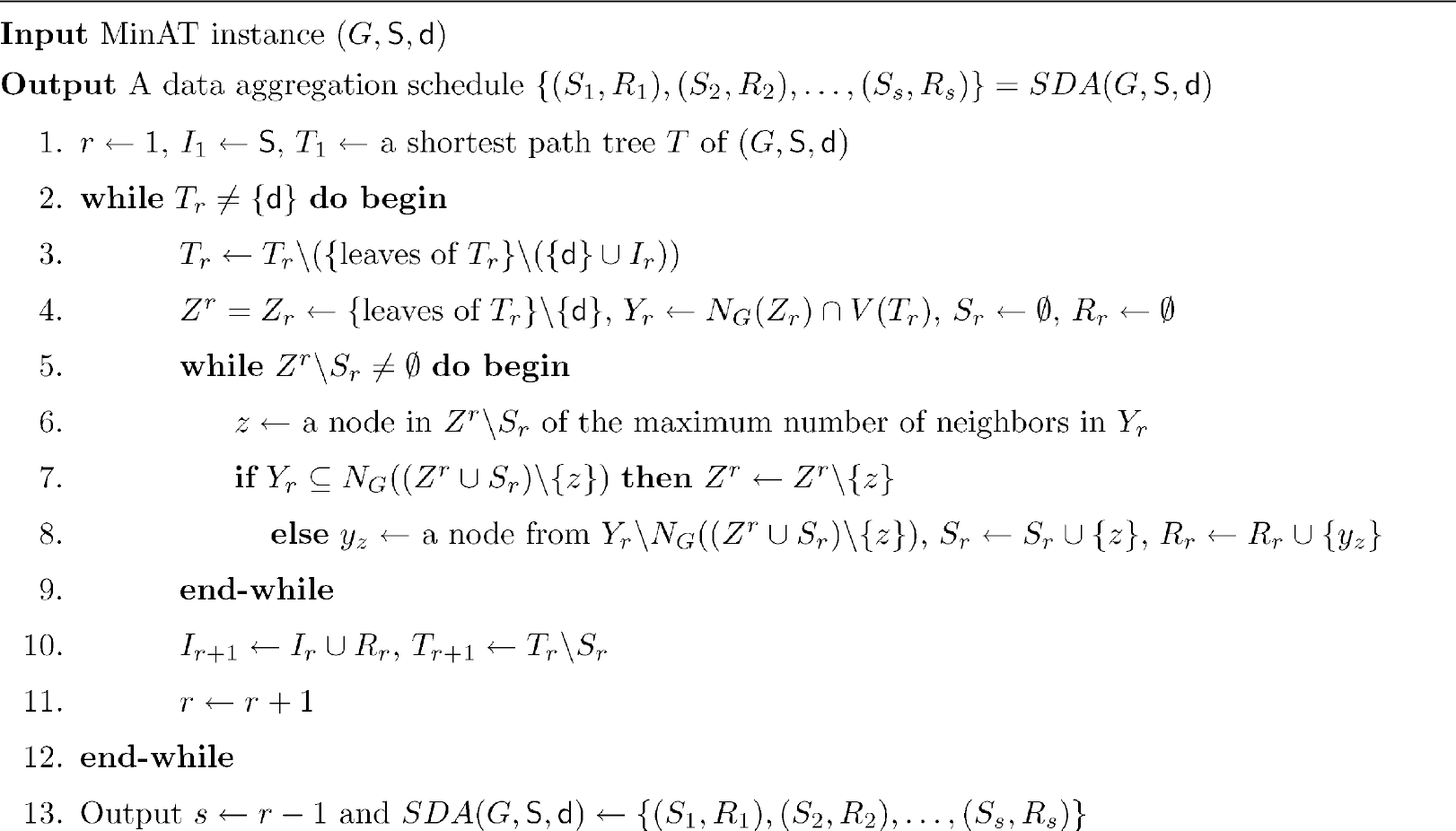
Algorithm SDA proceeds by incrementally constructing smaller and smaller shortest path trees rooted at d that span all nodes in S. It, initially, sets T₁ to a shortest path tree of (G, S, d). A number of iterations are implemented by SDA (refer to the pseudo-code below) and each iteration produces a schedule of a round. In the r-th iteration, T_r is a shortest path tree rooted at d spanning a set of nodes that possess all data aggregated from S till round r — 1. SDA selects from the leaves of T_i as the senders for round r. In Step 4–9, the variable Z_r with initial value {leaves of T_r}\{d} is used for selection. The set Z_r maintains the property that every non-leaf neighbor of a leaf in T_r other than d has a neighbor in Z_r. The leaves of T_r other than d are examined in the decreasing order of the number of their neighbors in G that are non-leaf node in T_r. A leaf is eliminated from Z_r if and only if the elimination does not destroy the property of Z_r. When all leaves of T_r other than d are examined, the remaining nodes in Z_r form the set S_r of the senders in round i. Subsequently, SDA eliminates S_r from its consideration by setting T_r+1 = T_r\S_r and ends the (r + 1)-th iteration. For a node set U in G = (V, E), the notation N_G(U) is a shorthand of ${v : u v \in E, u \in U}$ , and N_G({u}) is simply written as N_G(u).

Algorithm SDA Shortest_Data_Aggregation

One of the main ideas of our shortest-data-aggregation-based algorithms is to apply degree sorting and assign parallel transmissions (e.g., Step 5–9 of SDA). Intuitively speaking, we prefer to assign nodes of small degrees to send data before those of large degrees, and to arrange nodes of similar degrees to send data simultaneously. Both preferences increase potentially the number of parallel sendings/receivings and therefore reduce potentially the data aggregation time. Next we analyze theoretically the correctness and the performance of SDA.

Lemma 4.1

Let $R_{0} = S_{0} = Z_{s + 1} = \emptyset$ . All of the following hold for each r with $1 \leq r \leq s$ .

(i)
I_r consists of all informed nodes at the beginning of round r.
(ii)
T_r is a subtree of $T ∖ (⋃_{i = 0}^{r - 1} S_{i})$ with root d such that $| V (T_{r}) | \geq 2$ and all data on S\V(T_r) have been aggregated to nodes in V(T_r) at the beginning of round r (i.e. the end of round r — 1).
(iii)
Y_r and Z_r are nonempty subsets of V(T_r) such that $Y_{r} \subseteq N_{G} (Z_{r})$ .
(iv)
$Y_{r} \subseteq N_{G} (S_{r})$ in Step 10.
(v)
There is an 1-1 mapping between S_r and R_r in such a way that every sender z ∈ S_r corresponds to its receiver $y_{z} \in R_{r}$ .
(vi)
$S_{r} \subseteq Z_{r} \subseteq I_{r}, Z_{r} ∖ S_{r} \subseteq Z_{r + 1}, \emptyset \neq R_{r} \subseteq I_{r + 1} \cap Y_{r} \subseteq V (T_{r + 1}) \subseteq V (T_{r}) ∖ S_{r} T_{r}$

Proof

We apply inductive arguments on r. First we examine the base case in which r = 1. Statements (i)-(iii) are trivially true since T is a shortest path tree whose leaves must be all in S. Using $Y_{1} \subseteq N_{G} (Z_{1})$ , it is easily checked that in the $| Z_{1} |$ times implementations of the inter while-loop (Step 5–9), $Y_{1} \subseteq N_{G} (Z^{1})$ always holds, and $z \in Z_{1}$ is put into S₁ and y_z is put into R₁ if and only if $y_{z} \in N_{G} (z)$ and S₁ will not contain any neighbor of y_z other than z. Statements (iv) and (v) follow (note that Z¹ = S₁ ultimately in Step 10). Step 3 guarantees $S_{1} \subseteq Z_{1} \subseteq I_{1}$ , which in turn gives $Z_{1} ∖ S_{1} \subseteq Z_{2}$ . Since $\emptyset \neq Y_{1} \subseteq N_{G} (S_{1})$ (by (iii) and (iv)), we deduce from (v) that $| R_{1} | = | S_{1} | > 0$ . It is easily checked from Step 10 and Step 3 that (vi) holds.

Then we proceed to inductive steps. We check (i)–(vi) one by one for $2 \leq r \leq s$ under the hypothesis that (i)–(vi) are true for r — 1. For the simplicity of description, we use superscripts r — 1 and r to distinguish the conclusions (i)-(vi) with respect to r — 1 and r, respectively, i.e., (i)^r—1, (ii)^r—1, …, (vi)^t—1 and (i) ^r , (ii) ^r , …, (vi) ^r . Statement (i) ^r is true by (i)^r—1, (v)^r—1, (vi)^r—1, and $I_{r} = I_{r - 1} \cup R_{r}$ in Step 10. Since $S_{r - 1} (\subseteq Z_{r - 1})$ consists of some leaves of T_r—1 (by (vi)^r—1), T_r—1\S_r—1 is a tree, so is T_r in Step 10 and in Step 2. Moreover $| V (T_{r}) | \geq 2$ in Step 2. If all nodes other than d are deleted from T_r in Step 3, then $Z_{r} = \emptyset$ , and it follows from (vi)^r—1 that R_r—1 = {d} (by $R_{r - 1} \subseteq V (T_{r})$ ) and $\emptyset \neq V (T_{r - 1}) ∖ (S_{r - 1} \cup {d}) \subseteq Z_{r - 1} ∖ S_{r - 1} \subseteq Z_{r}$ , a contradiction. Thus we have $| V (T_{r}) | \geq 2$ in Step 4. Now (ii) ^r follows from (ii)^r—1, (vi)^r—1, (vi)^r—1, Step 3 and (i) ^r . Obviously, (iii) ^r follows from $| V (T_{r}) | \geq 2$ . Statements (iv) ^r -(vi) ^r can be justified by applying arguments similar to those used in the base case with script r in place of script 1.

Corollary 4.1

(i) S₁, S₂, …, S_s are pairwise disjoint. (ii) $S_{r} \cap (R_{r} \cup R_{r + 1} \cup \dots \cup R_{s}) = \emptyset$ for all $1 \leq r \leq s$ . (iii) T = T₁ T₂ … T_s T_s+1 = {d}.

Theorem 4.1

Given an instance (G, S, d) of MAT problem, Algorithm SDA produces a schedule in time of $O (| V |^{2} \log | V | + | V | | E |)$ .

Proof

The termination of SDA is guaranteed by Corollary 4.1 (iii). From T_s+1 = {d} and Lemma 4.1 (v) and (vi), it can be verified that T_s is a 2-node tree on R_s = {d} and it is the only sender in S_s. Since, by Lemma 4.1 (ii), all data on S have been aggregated to V(T_s) at the end of round s — 1, the schedule {(S₁, R₁), …, (S_s—1, R_s—1), (S_s, R_s)} output by SDA aggregates all data on S to d within s rounds.

To estimate the running time of Algorithm SDA, note that the computation of a SPT in Step 1 requires time $O (| V | + | E |)$ and SDA executes the external while-loop (Step 2–12) at most |V| times, i.e., s ≤ |V|. Since within the r-th iteration (of the external while-loop) sorting degree of nodes in Z^r and selecting nodes to form S_r can be accomplished in time $O (| V | \log | V |)$ and O(|E|), respectively, we deduce that the time complexity of SDA is $O (| V |^{2} \log | V | + | V | | E |)$ .

We now study the approximation performance ratio of Algorithm SDA. Denote h = h(G, S, d). Set L_i = {nodes in T at i hops away from d} for every 0 ≤ i ≤ h + 1; in particular, L₀ = {d} and L_h+1 = θ. Set T_i = θ for all i ≥ s + 2.

Lemma 4.2

$L_{h + 1 - i} \cap V (T_{(Δ - 1) i + 1}) = \emptyset$ for every 0 ≤ i ≤ h — 1, where Δ is the maximum degree of G.

Proof

The proof is by induction on i. The base case where i = 0 is justified by $L_{h + 1} = \emptyset$ . Proceeding inductively, suppose that $j = (Δ - 1) (i - 1) + 1$ and $L_{h + 1 - (i - 1)} \cap V (T_{j}) = \emptyset$ , which implies that any node in $L_{h + 1 - i} \cap V (T_{j})$ is a leaf in T_j. We aim to show $L_{h + 1 - i} \cap V (T_{j + Δ - 1}) = \emptyset$ . By contradiction, let $v \in L_{h + 1 - i} \cap V (T_{j + Δ - 1})$ . Note from Step 4 (the definition of Z_r) and Lemma 4.1 (vi) that v $v \in Z_{j + k}$ for every 0 ≤ k ≤ Δ − 1. Hence there exists $u \in L_{h - i}$ such that $u \in Y_{j + k}$ for every 0 ≤ k ≤ Δ — 1. It follows from Lemma 4.1 (iv) and Corollary 4.1 (i) that there exist Δ distinct nodes v₀, …, v_Δ—1 such that $v_{k} \in S_{j + k} \cap N_{G} (u)$ for $k = 0, \dots, Δ - 1$ . Recall from Lemma 4.1 (ii-iii) that $S_{j + Δ - 1} \cap Y_{j + Δ - 1} = \emptyset$ and u is a node in tree $T_{j + Δ - 1} ∖ S_{j + Δ - 1}$ . Observe that $d \in V (T_{j + Δ - 1}) ∖ S_{j + Δ - 1}$ and $u \neq d$ (since i ≤ h — 1). Therefore u has a neighbor w in $T_{j + Δ - 1} ∖ S_{j + Δ - 1}$ . Now u has Δ + 1 distinct neighbors w, v₀, …, v_Δ—1. The contradiction completes the proof.

Theorem 4.2

Given any instance (G, S, d), Algorithm SAD produces a schedule whose data aggregation time t_SDA (G, S, d) ≤ min{(Δ — 1)h + 1, (Δ — 1)t_OPT(G, S, d)}.

Proof

To prove the theorem, it suffices to show (i) |t_SDA(G, S, d)| ≤ (Δ — 1)h + 1 and (ii) |t_SDA(G, S, d)| ≤ (Δ — 1)T_OPT(G, S, d). Recall from Lemma 2.1 that t_OPT(G, S, d) ≥ h. If s = |SDA(G, S, d)| ≤ (Δ — 1)(h — 1) + 1 then we are done. So we assume s >(Δ — 1)(h — 1) + 1.

To justify (i), we deduce from Lemma 4.2 that $L_{2} \cap V (T_{(Δ - 1) (h - 1) + 1}) = \emptyset$ , and then from Lemma 4.1 (ii) that $V (T_{(Δ - 1) (h - 1) + 1}) \subseteq L_{1} \cup {d}$ . Note that |L₁| ≤ Δ and T_s+1 = {r}. Thus by Corollary 4.1 (iii) we obtain s + 1 ≤ (Δ — 1)(h — 1) + 1|L₁| ≤ Δ(h — 1) + 2, which implies (i).

Next we prove (ii). In case of |L_h| ≥ 2, we have t_OPT(G, S, d) ≥ h + 1 and (i) implies s ≤ (Δ — 1)t_OPT(G, S, d). It remains to consider the case where |L_h| = 1. We may assume Δ ≥ 3 (since otherwise, G is a path or a cycle and s = h = t_OPT(G, S, d)). It is obvious that S₁ = L_h. Let G′ = G\L_h and S' consist of the nodes in S\L_h and the neighbor (parent) of L_h in T. Then T\L_h is a shortest path tree of (G′, S′, r) that has height h — 1; moreover, there is an implementation of SDA on (G′, S', d) which outputs {S′₁, S′₂, …, S′_s—1} with S′_i = S_i+1 for all 1 ≤ i ≤ s — 1. Using (i), we have s — 1 = |t_SDA(G′, S′, d)| ≤ (Δ — 1)(h — 1) + 1 since the maximum degree of G′ is upper bounded by Δ. It follows from Δ ≥ 3 that s ≤ (Δ — 1)h ≤ (Δ — 1)t_OPT(G, S, d), and (ii) is proved.
4.2. Algorithms for Special Cases

In this subsection, we show that, when Algorithm SDA is applied to some special instances of the MAT problem, it will produce solutions with better theoretical guarantees. First, in view of Theorem 4.2, SDA provides a (Δ — 1)-approximation for UDGs with maximum degree Δ. In a realistic situation, sensor devices cannot be too close or overlapped; thus it is reasonable to assume that the distance between any two nodes is no less than a positive constant λ. The UDG modelling such a sensor network is called a λ-precision unit disk graph [?], [14]. Krumke et al. [15] showed that the maximum degree of a λ-precision UDG is at most [2π/λ²]. Consequently, we have the following result.

Corollary 4.2

Given any instance (G, S, d) with λ-precision G, Algorithm SAD produces a schedule whose data aggregation time $t_{S D A} (G, S, d) \leq \frac{2 π}{λ^{2}} t_{O P T} (G, S, d)$ .

Next we exhibit some local properties of UDGs, which ensure that Algorithm SDA has a better performance guarantee in some other special cases. Let v be a node in a UDG G =(V, E) of degree d. Then all nodes in N_G(v) = {v₀, …, v_d—1} are located within a disk centered at v with radius 1 and boundary B of length 2π. Corresponding to every v_i(0 ≤ i ≤ d — 1), let b_i be a point on B such that ||b_i — v_i|| is minimized. If ||v_i — v_j||>1, then the angle between the ray originated at v through v_i, b_i and the ray originated at v through v_i, b_i and the ray originated at v through v_j, b_j is greater than π/3. This implies ||b_i — b_j||>1. Thus

l_{i, j} \leq π / 3 \Rightarrow ∥ b_{i} - b_{j} ∥ \leq 1 \Rightarrow ∥ v_{i} - v_{j} ∥ \leq 1, for any 0 \leq i, j \leq d - 1,

(1)

where l_{i, j} denotes the length of the clockwise arc in B from b_i to b_j.

Lemma 4.3

Let G =(V, E) be a planar UDG. Then its maximum degree Δ ≤ 15.

Proof

Let $v \in V$ be a node in G of the maximum degree Δ. Denote N_G(v) = {v₀, …, v_Δ—1} and let b₀, …, b_Δ—1 be Δ points on the boundary B of the unit disk centered at v that minimize ||b_i — v_i||, i = 0, …, Δ — 1. As usual, K_k stands for a complete graph on k vertices, and a subdivision of K₅ is the graph obtained from a K₅ by replacing each edge e of the K₅ with a path between the ends of e whose internal nodes (if any) all have degree 2. The planarity of G implies that

\begin{aligned} the subgraph induced by {v} \cup N_{G} (v) contains no subdivision of K_{5}; \\ and in particular no four nodes in N_{G} (v) can induce a K_{4} . \end{aligned}

(2)

If an arc in B of length at most π/3 contains four distinct points $b_{i}, b_{j}, b_{k}, b_{ℓ}$ , then the distance between every pair from ${b_{i}, b_{j}, b_{k}, b_{ℓ}}$ is not greater than 1, so is the distance between every pair from ${v_{i}, v_{j}, v_{k}, v_{ℓ}}$ by (1); it follows that ${v_{i}, v_{j}, v_{k}, v_{ℓ}}$ induces a K₄ contradicting (2). Hence

any arc in B of length π / 3 can contain at most three points from b_{0}, \dots, b_{Δ - 1} .

(3)

To see Δ ≤ 15, assuming the contrary Δ ≥ 16, we consider v_i, b_i, i = 0, 1, …, 15, and do all additions involving subscripts in modulo 16. Without loss of generality suppose that b₀, …, b_Δ—1 are on B in clockwise order. It is instant from (3) that

l_{i, i + 3} > π / 3 for every 0 \leq i \leq 15.

(4)

If l_i,i+1 > π/3 for some i, then (4) implies a contradiction $2 π \geq l_{i, i + 1} + (l_{i + 1, i + 4} + l_{i + 4, i + 7} + l_{i + 7, i + 10} + l_{i + 10, i + 13} + l_{i + 13, i}) > π / 3 + 5 (π / 3)$ . So l_i,i+1 ≤ π/3 and therefore (1) implies that

G contains a cycle C with V (C) = {v_{0}, v_{1}, \dots, v_{15}} .

(5)

Similarly, if both $l_{i, i + 2} > π / 3$ and $l_{i + 2, i + 4} > π / 3$ for some i, then the contradiction $2 π \geq l_{i, i + 2} + l_{i + 2, i + 4} + (l_{i + 4, i + 7} + l_{i + 7, i + 10} + i_{i + 10, i + 13} + l_{i + 13, i}) > π / 3 + π / 3 + 4 (π / 3)$ is also implied by (4). Thus

min {l_{i, i + 2}, l_{i + 2, i + 4}} \leq π / 3 for every 0 \leq i \leq 15.

(6)

If $l_{i, i + 2} \leq π / 3$ and $l_{i + 1, i + 3} \leq π / 3$ for some i, then $C \cup {v} \cup {v v_{i}, v v_{i + 2}, v v_{i + 3}, v_{i} v_{i + 2}, v_{i + 1} v_{i + 3}}$ is a subdivision of K₅ in G, a contradiction to (2). So

max {l_{i, i + 2}, l_{i + 1, i + 3}} > π / 3 for every 0 \leq i \leq 15.

(7)

By (6), suppose without loss of generality that $l_{0, 2} \leq π / 3$ . We then have the following implications $l_{0, 2} \leq \frac{π}{3} (7) \Rightarrow l_{1, 3} > \frac{π}{3} (6) \Rightarrow l_{3, 5} \leq \frac{π}{3} (7) \Rightarrow l_{4, 6} > \frac{π}{3} (6) \Rightarrow l_{6, 8} \leq \frac{π}{3} (7) \Rightarrow l_{7, 9} > \frac{π}{3} (6) \Rightarrow l_{9, 11} \leq \frac{π}{3} (7) \Rightarrow l_{10, 12} > \frac{π}{3} (6) \Rightarrow l_{12, 14} \leq \frac{π}{3} (7) \Rightarrow l_{13, 15} > \frac{π}{3} (6) \Rightarrow l_{15, 1} \leq \frac{π}{3} (7) \Rightarrow l_{0, 2} > \frac{π}{3}$ . The contradiction establishes the result.

Corollary 4.3

Algorithm SDA produces a schedule to the MAT problem within approximation ratios 3 for grid graphs, 14 for planar UDGs, and $\sqrt{12 | E |}$ for general UDGs.

Proof

The first two bounds come directly from Theorem 4.2 and Lemma 4.3 immediately. We prove the third bound by showing $Δ - 1 \leq \sqrt{12 | E |}$ . To this end, consider a node v in UDG G of maximum degree Δ and the boundary B of the unit disk centered at v. We may partition N_G(v) = {v₀, …, v_Δ—1} into six disjoint subsets V₁, V₂, …, V₆ such that ${b_{j}; v_{j} \in V_{i}}$ is contained by an arc in B of length π/3. By (1), each $V_{i} \cup {v} (1 \leq i \leq 6)$ induces a $K_{| V_{i} | + 1}$ in G. It follows that $\sum_{i = 1}^{6} | V_{i} | = Δ$ , and the number of edges in the subgraph of G induced by ${v} \cup N_{G} (v) = {v} \cup (⋃_{i = 1}^{6} V_{i})$ is lower bounded by

\sum_{i = 1}^{6} \frac{| V_{i} | (| V_{i} | + 1)}{2} = (\sum_{i = 1}^{6} \frac{| V_{i} |^{2}}{2}) + \frac{Δ}{2} \geq \frac{1}{12} {(\sum_{i = 1}^{6} | V_{i} |)}^{2} + \frac{Δ}{2} = \frac{Δ^{2}}{12} + \frac{Δ}{2},

which implies |E| > Δ²/12. Hence

Δ - 1 \leq \sqrt{12 | E |}

5. Simulation

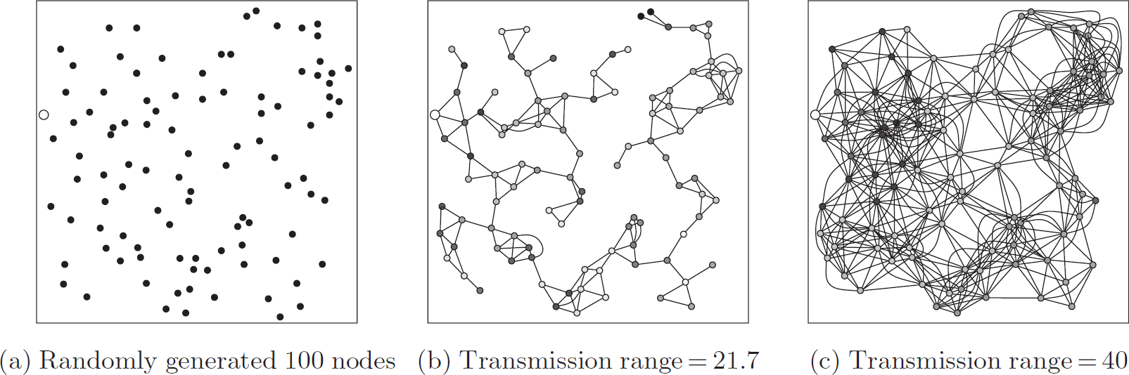
Establishment of a sensor network can be carried out in either a random way (e.g., dropped from an airplane) or a nonrandom way (e.g., fire alarm sensors in facility). In the latter case, WSNs have nice properties including bounded-degree; consequently our theoretical results assure satisfactory approximation for the MAT problem. Thus we focus on the former case and use 100-node network shown in Fig. 2a as our test network. This network was randomly generated within a 200 × 200 square region. The sink d is selected to be the leftmost node (the larger white node in Fig. 2) among the 100 nodes. We use a similar simulation technique to that in [16]. In our simulations, the transmission range varies from 21.692 to 40 so that the number of edges of the UDG modelling the WSN varies from 167 to 546 (see Fig. 2b and c), where 21.692 is the minimum transmission range that guarantees the network to be connected. The variations of other parameters are summarized in Table 1. To evaluate the proposed algorithm SDA we compare its performance t_SDA with that of convergecast algorithm in [5], denoted by t_AGS.

Figure 2.

Randomly generated WSNs used in simulation.

Table 1

Graph parameters and convergecasting times

Transmission range	m	Δ	h	t_SDA	t_AGS
21.692	167	6	27	28	50
25	223	8	13	18	32
30	318	10	12	19	38
35	417	14	8	18	38
40	546	16	7	21	38

m: the number of edges Δ: the maximum degree.

h: the height of the bread first search tree with root d.

It can be observed from Table 1 and Fig. 3 that SDA has a performance much better than the other algorithm. Moreover, the ratio of t_SDA to h is much less than the theoretical performance ratio Δ — 1. This highlights the advantages of assigning parallel transmissions according to degree order in our shortest-data-aggregation-based algorithm SDA.

Figure 3.

Comparison of performances.

6. Conclusion

In this paper we have studied the MAT problem aiming for time-efficient data aggregation in WSNs. We first prove the problem is NP-hard even for some special cases, and then propose an approximation algorithm for the problem with provable performance guarantee.

In order to achieve both time-efficiency and energy-efficiency, we can implement our shortest data aggregation algorithm in such a way that it saves more energy at the expense of a small increase of data aggregation time. Given a MAT instance (G, S, d), a tree of G spanning $S \cup {d}$ with a minimum number of edges c(G, S, d) is called a minimum Steiner tree of (G, S, d). Let α and β be two constants satisfying β ≥ 2 + 4/(α — 1). Applying Kuller-Raghavachari-Young algorithm [17] we can find a tree T of G spanning $S \cup {d}$ such that the height of T is at most αh(G, S, d) and the number of edges of T is at most βc(G, S, d). Let E_SDA be the variation to SDA that takes T₁ in Step 1 as a tree produced by the Khuller-Raghavachari-Young algorithm. Then E_SDA outputs a data gathering schedule whose data aggregation time is at most α(Δ — 1)h(G, S, d) ≤ (Δ — 1)t_OPT (G, S, d) with energy cost at most β times the optimal one.

In our work we assume that all sensor nodes have the same transmission range. For future work it would be interesting to study the case with adjustable transmission ranges. In addition, it is worthy of studying how to deal with 3-dimensional cases.

Footnotes

Appendix

Proof of Lemma 3.1. By Lemma 3.1, the orthogonal planar embedding stated below is derived in time polynomial in g.

H has an orthogonal planar drawing D of grid size gXg in which every edge of H has at most 2 bends.

An orthogonal planar drawing D′ of H with grid size (40g² + 40g) X (40g² + 40g) can be obtained from D in a direct way that point (x, y) in D maps to point (40nx, 40ny) in D′, and every vertical (resp. horizontal) segment of unit length (segment for short) in D maps to a vertical (resp. horizontal) path of length 40g in D′ between the images (in D′) of the ends of the segment (in D). (The additional 40g is set for the further modification on the drawing.) It is straightforward from (a) that

each edge of H has length at most 120g² in D′.

We propose to modify D′ into an orthogonal planar drawing of H′ with grid size (40g² + 40g) X (40g² + 40g) in which every edge of H′ is a vertical or horizontal segment and any two nonadjacent vertices of H′ are drawn on two points with distance at least two. To this end, we consider a 18gx18g grid K and a, b the two corners of K on one side. We call a path from a to b an a-b path.

For every even integer j with 18g ≤ j ≤ 120g², K contains an a-b path P_j of length j which is a UDG.

Without loss of generality suppose that a and b are located on (0, 0) and (18g, 0), respectively. Let $k \in {18 g, 18 g - 2}$ be such that k/2 + 1 is an even number (i.e. {0, 2, 4, …, k} is of even size). Denote by I_2i (0 ≤ i ≤ k/2) the path consisting of points and segments on the 2i-th (vertical) column of K. For each 0 ≤ i ≤ k — 6 which is a fold of 4, let J_i (resp. J_i+2) be the shortest path connecting the top ends of I_i and I_i+2 (resp. the bottom ends of of I_i+2 and I_i+4) and let J_k—2 (resp. J_k) be the shortest path connecting the top ends of I_k—2 and I_k (resp. the bottom end of I_k and b). Thus J₀, J₂, J₄, …, J_k—2 are all horizontal paths of length 2, J_k is horizontal paths of length 0 (when k = 18g) or 2 (when k = 18g — 2), and J₀, J₄, …, J_k—2 (resp. J₂, J₆, …, J_k—4, J_k) are contained in the top (resp. bottom) row of K. Now we get an a-b path $P_{l} := ⋃_{i = 0}^{k / 2} (I_{2 i} \cup J_{2 i})$ of even length $ℓ > (k / 2 + 1) 18 g > 120 g^{2}$ . Clearly $P_{ℓ}$ is induced, and so is a UDG. Inductively, suppose that K contains an a-b path P_j of even length j(≥ 18g + 2) such that P_j is a UDG containing $J_{2} \cup J_{6} \cup \dots \cup J_{k - 4} \cup J_{k}$ , and all vertical segments of P_j are contained in $⋃_{i = 0}^{k / 2} I_{2 i}$ . Since j ≥ 18g + 2, we see the statement holds for j — 2 in a way that P_j—2 is obtained from P_j by replacing a subpath of P_j of length 4 consisting of two vertical segments and two horizontal segments with a horizontal path in K of length 2 between the same ends. Consequently, statement (c) is proved by induction.

We turn back to the drawing D′ Consider an arbitrary edge e of H of length $ℓ_{e}$ in D′. Let S_e be the subpath (in the (40g² + 20g) X (40g² + 40g) grid) of the drawing of e consisting of a maximal sequence of vertical (or horizontal) segments. Let u_e and b_e be the ends of S_e such that the summation of coordinates of u_e is less than the summation of coordinates of b_e. Then

In D′, point u_e (resp. b_e) is a bend or an end of e, and S_e is a vertical or horizontal path of even length at least 40g.

Now we put a 18gX18g grid K_e such that $K_{e} \cap S_{e}$ is an a_e-b_e path L_e which is a side of K_e, and $∥ a_{e} - b_{e} ∥ > ∥ b_{e} - b_{e} ∥ = 2$ . By (a) and (b), let P_e be the a_e-b_e path in K_e of length $120 g^{2} - ℓ_{e} + 18 n$ which is a unit disk graph. Construct drawing D″ from D′ by replacing each L_e in S_e with P_e in K_e. Let H′ be the graph whose vertex (resp. edge) set consists of all points (resp. segments) in D″ Then D′ is an orthogonal planar drawing of G′ of grid size (40g² + 40g) X (40n² + 40g) and G′ is a graph obtained from G by replacing each edge of G with a path of length 120g². Moreover

In the embedding D″ of H′ the distance between any point (vertex) in P_e\{a_e, b_e} and any point (vertex) in H′\V (K_e) is at least two.

Suppose the contrary that cc ∈ V(P_e) — {a_e, b_e} and n ∈ V(H′) — V(K_e) has distance one in D″. Since any two vertical (resp. horizontal) segments in D′ have distance at least 40g, it follows from (c) and $∥ a_{e} - b_{e} ∥ > ∥ b_{e} - b_{e} ∥ = 2$ that n∈ P_f for some other edge f of H. From the positions of K_e on S_e and K_f on S_f, we deduce that S_e or S_f has length less than 40g, a contradiction to (d). Hence (e) holds.

Combining (c) and (e), we conclude that H′ is a UDG and establish the lemma.

References

Imielinski

and Goel

, “DataSpace: querying and monitoring deeply networked collections in physical space,” IEEE Personal Communications, vol. 7, pp. 4–9, 2000.

Bulusu

, Heidemann

, and Estrin

, “GPS-less low cost outdoor localization for very small devices,” Computer Science Department, University of Sourthern California, Tech. Report 00–729, April 2000.

Kalpakis

, Dasgupta

, and Namjoshi

, “Efficient algorithms for maximum lifetime data gathering and aggregation in wireless sensor networks,” in Proceedings of the International Journal of Computer and Telecommunications Networking, vol. 42, 2003, pp. 697–716.

H.-W.

, Hu

X.-D.

, and Jia

X.-H.

, “Energy efficient routing and scheduling for real-time data aggregation in WSNs,” Computer Communications, vol. 29, pp. 3527–3535, 2006.

Annamalai

, Gupta

S. K. S.

, and Schwiebert

, “On tree-based convergecasting in wireless sensor networks,” in Proceedings of the IEEE Wireless Communication and Networking Conference, 2003, pp. 1942–1947.

Kesselman

and Kowalski

, “Fast distributed algorithm for convergecast in ad hoc geometric radio networks,” in Proceedings of the 2nd Annual Conference on Wireless On-demand Network Systems and Services, 2005, pp. 119–124.

Garey

M. R.

and Johnson

D. S.

, Computers and Intractability: A Guide to the Theory of NP-Completeness, Freeman, San Francisco, 1979.

Ravi

R. R.

, “Rapid rumor ramification: approximating the minimum broadcast time,” In Proceedings of the 35th Annual IEEE Symposium on Foundations of Computer Science, 1994, pp. 202–213.

Bar-Noy

, Guha

, Naor

, and Schieber

, “Message multicasting in heterogeneous networks,” SIAM Journal on Computing, vol. 30, pp. 347–358, 2000.

10.

Gandhi

, Parthasarathy

, and Mishra

, “Minimizing broadcasting latency and redundancy in ad hoc networks,” in Proceedings of the 4th ACM International Symposium on Mobile Ad Hoc Networking and Computing, 2003, pp. 222–231.

11.

Biedl

and Kant

, “A better heuristic for orthogoanl graph drawings,” Computational Geomety, vol. 9, pp. 159–180, 1998.

12.

Lichtenstein

, “Planar formulae and their uses,” SIAM Journal on Computing, vol. 11, pp. 329–343, 1982.

13.

Di Battista

, Liotta

, and Vargiu

, “Spirality of orthogonal representations and optimal drawings of series-parallel graphs and 3-planar graphs,” in Proceedings of Workshop on Algorithms and Data Structures, Lecture Notes in Computer Science, vol. 709, Springer, New York, 1993, pp. 151–162.

14.

Hunt

H. B.

III , Marathe

M. V.

, Radhakrishnan

, Ravi

S. S.

, Rosenkrantz

D. J.

, and Stearns

R. E.

, “NC-approximation schemes for NP- and PSPACE-hard problems for geometric graphs,” Journal of Algorithms, vol. 26, pp. 238–274, 1998.

15.

Krumke

S. O.

, Marathe

M. V.

, and Ravi

S. S.

, “Models and approximation for channel assignment in radio networks,” Wireless Networks, vol. 7, pp. 575–584, 2001.

16.

Varshnery

and Bagrodia

, “Detailed models for sensor network simulations and their impact on network performance,” in Proceedings of the 7th International Symposium on Modeling Analysis and Simulation of Wireless and Mobile Systems, 2004, pp. 70–77.

17.

Khuller

, Raghavachari

, and Young

, “Balancing minum spanning trees and shortest path trees,” Algorithmica, vol. 14, pp. 305–321, 1995.

Data Gathering Schedule for Minimal Aggregation Time in Wireless Sensor Networks

Abstract

Keywords

1. Introduction

2. Preliminaries

2.1. Model Description

Lemma 2.1

2.3. Our Contributions

3. Complexity Analysis

Lemma 3.1

Lemma 3.2

Theorem 3.1

Proof

4.1. Basic Algorithm

Lemma 4.1

Proof

Corollary 4.1

Theorem 4.1

Proof

Lemma 4.2

Proof

Theorem 4.2

Proof

Corollary 4.2

Lemma 4.3

Proof

Corollary 4.3

Proof

Footnotes

Appendix

References