
Abstract
We propose to develop Wireless Sensor Networks with Mobile Sinks (MSSN), under high sensor node density, where multiple sensor nodes need to share one single communication channel in the node-to-sink transmission. By exploiting the tradeoff between the successful information retrieval probability and the nodes energy consumption, a number of multiple nodes transmission scheduling algorithms are proposed. Both optimal and suboptimal algorithms, which exhibit exponential and linear complexity respectively, are discussed under the desired application. Computer simulations show that suboptimal algorithms perform nearly as good as the optimal one. The study leads to the cross-layer Wireless Link layer design for MSSN.
Keywords
Introduction
The unique nature of wireless sensor networks, which are resource-limited and application-specific, requires new approaches in the system design. Recently [1], we proposed to develop Sensor Networks with Mobile Sinks (MSSN) for two application areas, environment monitoring systems with high latency tolerance [19], and intelligent-space [17]. This new architecture features very high energy-efficiency, because multi-hop transmissions of high volume data over the network is converted to single-hop transmissions. Additional advantages of MSSN include: infrastructure free, high security, and ease of implementation. In [1], we discussed the transmission scheduling algorithm TSA-MSSN in a sparsely deploying network setup, where it is assumed that only one sensor node is communicating with the mobile sink on a given channel.
However, when the density of sensor networks increases, multiple nodes can be within the transmission range to the sink, and the assumption of a sparsely deploying setup no longer holds. Consider for example the application of micro spies [5]. A micro spy is a micro aircraft with the size of less than six inches. For the purpose of battlefield observation and strategic reconnaissance, sensor networks can be deployed in a remote place with limited wireless infrastructures. A micro spy can, on the other hand, act as a mobile sink, which flies over the sensor deployed region and delivers the collected information back to the commander. In the communication setup, a number of sensor nodes need to send packets to the micro spy simultaneously, because of the importance of the desired information. Also, it may be risky to have the micro spies stay in the air for too long a time, hence, the communication time slots available are limited.
The wireless architecture in this scenario is centralized, which is analogous to cellular networks, star network setup in IEEE 802.15.4 [6], and Point Coordination Function (PCF) in IEEE 802.11 [7]. Although there is a large number of classical multiple access schemes [15] available, such as TDMA, FDMA, CDMA, etc., all of them assume that multiple wireless channels are available for node-to-sink communication. In our case, the sink can assign one such distinctive channels to any individual node. The TSA-MSSN, proposed in [1], can then operate on different channels respectively. However, when the number of nodes exceeds the number of channels, multiple nodes will need to share one channel. Thus, multiple nodes scheduling algorithms are needed to ensure the Quality of Service (QoS) of the wireless network.
Under different types of wireless networks, there are numerous works investigating the desired scheduling problem. Under cellular networks, from an information theoretic approach, [8] showed that, to maximize the total uplink capacity, it is sufficient to have only the user with the strongest channel to the base station transmit at any given time. Such a power control scheme is known as multiuser diversity, which is also extended to downlink channels in [9], and other forms of channel capacity such as delay-limited capacity [10] and outage capacity [11]. Although strategies in [8] are optimal in the sense of capacity, in the service layer implementations, more QoS factors should be considered, such as fairness, delay, and connection admission control (CAC). Recent references on this topic can be found in CDMA cellular networks [12] and IEEE 802.11 enabled home networking [13]. In the area of sensor networks, SENMA [20] (Sensor Networks with Mobile Agents) studied the sensor network topology similar to MSSN, and proposed distributed random access scheduling. However, SENMA assumes a simple reachback sensor network, which differentiates it from the proposed MSSN.
Compared to the existing works, the MSSN is distinctive for the following reasons: In MSSN, the objective of scheduling algorithms is to retrieve integrated/compressed information [14] stored on sensor nodes with the minimum energy consumption. Combined with the mobility of the sink, this guideline, [1], makes the system design different from the conventional wireless networks. More specifically, in the MSSN transmission scheduling, we exploit the tradeoff between the successful information retrieval credit and the nodes energy consumption cost, under the latency limitations imposed by the sink mobility. Instead, in conventional wireless networks, “throughput” is usually emphasized, which is the number of retrived packets per second.
Next, we discuss the scenario where multiple sensor nodes are sharing one communication channel in sending information to the mobile sink which is travelling through the deployed sensor networks. The system description is provided in Section II. The proposed optimal multiple nodes transmission scheduling algorithm (MTSA-MSSN) is described in Section III. The optimal MTSA-MSSN has the complexity which grows up exponentially with the number of nodes N. Thus, in Section IV, we propose suboptimal algorithms with the complexity as low as O(N). A comparison and validation of the suboptimal algorithms performance are given in Section V, by means of computer simulations. Discussions and concluding remarks are given in Section VI and VII, respectively.
System Description
Concepts and Assumptions
The concept of the scheduling design is to reduce the sensor nodes energy consumption, in the process of information retrieval, by exploiting the sink mobility. Utilizing the higher energy, computing, and storage resources at the sink, the proposed scheduling algorithms are centralized, and executed solely at the sink. The problem of finding the optimal scheduling policy is formulated as a Markov Decision Process (MDP), and solved in the framework of dynamic programming [22]. Essentially, the tradeoff between the successful information retrieval credit and the sensor nodes energy consumption cost is explored.
Let N denote the number of nodes sharing one specific communication channel. Assume that the location and the number of residual packets of every node are known at the sink, by a registration procedure. More specifically, the registration can be conducted on a separate control channel, where the nodes send the registration, i.e, the location and the packet number, upon the detection of the sink arrival, by means of carrier sensing multiple access (CSMA). The sink acknowledges the registration by assigning the node a generated identification number.
At the current time slot i0, the problem to formulate is how the sink decides the transmission strategy, i.e., which one of the N nodes is going to transmit and what is the transmission power. The scheduling algorithm is executed at the beginning of every communication time slot. One time slot is composed of the transmission of two different packets in sequence, which are the acknowledgement (ACK) packet from the sink, and the data packet from one of the sensor nodes, respectively. The obtained scheduling strategy can be piggybacked on the ACK packet broadcasted by the sink to the N associated sensor nodes. The ACK packet, on the other hand, also serves to acknowledge successful or failed data transmission in the previous time slot. It is assumed that the lost data packets will be retransmitted.
Assume that the sink has an estimation of its current mobility, which can be obtained from the Global Positioning System (GPS). We do not assume that the future mobility pattern is available at the sink. Instead, we make two approximations:
No new node is admitted to the channel until all N nodes have finished the transmission; The mobility of the sink is maintained constant in future time slots.
Both assumptions are realistic, because the scheduling algorithm is run at the beginning of every time slot, where both the nodes and the sink mobility information are updated.
In the scheduling design, we do not consider the possibility of new data arrival at sensor nodes, in the procedure of information retrieval. The sensor nodes is dissociated with the sink, whenever all the data packets have been retrieved.
System State Vector Ě(i 0 )
Let Range denote the communication range of the sensor node. It is assumed that Range is the same for all nodes. Let {

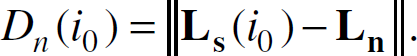
Let Dn(i0) denote the distance between the sink and the sensor node n, n = 1…N,
The communication channel gain for the node n can be modeled as [16].

where A is a constant decided by the antenna gain; β is the path loss exponent decided by the propagation environment, e.g. β = 2 for free space; and ξ is a random variable under normal distribution
Let Tn(i0) denote the estimated transmission time slots available for node n, n = 1…N. Since the sink is assumed to have constant mobility when passing through all the N circular regions, centered at {
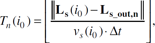
where
Let,

Then, the vector of estimated states can be defined as,

where Ě(i0) is known as,

and,

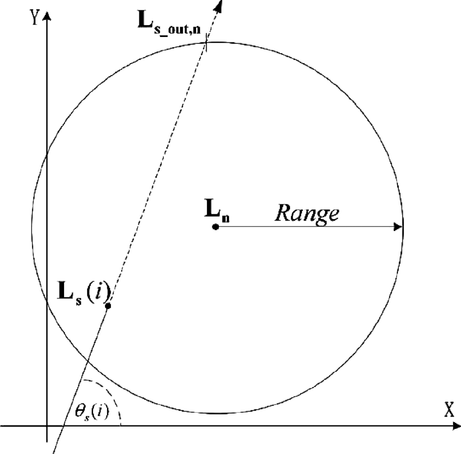
The mobile sink passes through the circular region centered on
Thus, the only variable parameters of each estimated state {Ě(i), i0 < i i0 + T(i0) + 1} are
The transmission strategy

where η(i) ∊ {1…N} denotes the ID of the transmitting node in time slot i. Pt(i) is, on the other hand, the transmission power at the sensor node η(i). Note that Pt(i) can be 0 if all N nodes are forced to sleep. We assume the discrete levels transmission power, and that the number of optional levels is Sizeof {Pt}. Given Ě(i) and

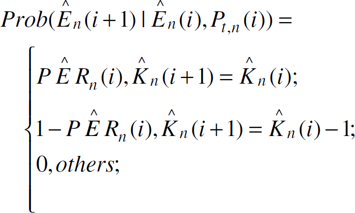
The state transferring probability function can be written as,

where PĚR(i) is the packet error rate of transmission in time slot i. Consider a BPSK modulated uncoded data packet. And assume that the sink is unaware of the shadowing effect ξ, i.e. in the channel model Eq. (3). Then, the PĚR(i) can be written as, [15],

where
In the definition of the transmission strategy
At current time i0, the objective of the MTSA-MSSN is to decide the optimal strategy

For i0 i i0 + T(i0), we define,

In Eq. (14), Jm (
Since {Ě(i)} is modeled as a Markov chain, there is:

and,

where max{Pt} is the maximum available RF (Radio Frequency) transmission power and acts as a normalization factor in Jc.
Thus, by combining Eq.(14,15,16), the function J can be written recursively as,

At the final state of the algorithm, i = i0 + T(i0) + 1, the utility function is decided only by Ě(i0 + T(i0) + 1), that is,

The definition of J (Ě(i0 + T(i0) + 1)) is, however, application dependent. For example, assuming that each packet is equally credited, say “1”, then it can be defined as,

If we set λ = 1 in Eq. (14), Eq. (19) suggests that the cost of a maximal power transmission time slot equal to the credit of successfully transmitting one packet.
As such, the optimal MTSA-MSSN can be solved by means of dynamic programming, and is summarized in Table 1. Compared with the TSA-MSSN [1], the size of strategy space in MTSA-MSSN has increased N times, from
Optimal MTSA-MSSN Algorithm

Moreover, the size of the state space 
Due to the fact that
Moreover, if a continuous power level control is implemented, the concavity of the utility function is only proved under the condition N = 1, [1]. It is unclear whether a computational simple way can be found for the optimization in Eq. (17), when N > 1.
Since the optimal algorithm has the complexity, C(Optimal) given by Eq. (20), which increases exponentially with the number of nodes N, it is infeasible for implementation on a mobile sink, such as a “micro spy.” In developing suboptimal algorithms, the idea is to run the TSA-MSSN (i.e. N = 1) algorithm individually for each node n, and combine the N individual strategies. We denote this suboptimal multiple-access transmission strategy as 
We outline the preprocessing procedure of TSA-MSSN for the integrity of this paper. Assume the current time slot is i0. Let Pt,n(i) denote the strategy (transmission power) of TSA-MSSN run on node n, and let Ě
n
(i) denote the estimated system state on node n, which is,

The definition of
The TSA-MSSN searches the maximum of a utility function 
The utility function for each node n, Jn, is recursively defined as,

where,
And,

assuming that BPSK modulated uncoded signal is transmitted.
The final state configuration function is Jn (Ě
n
(i0 + Tn(i0) + 1)). In compliance with Eq. (19), it is defined as,

Suboptimal MTSA-MSSN Algorithm Preprocessing

Table 2 summarizes the TSA-MSSN preprocessing in suboptimal algorithms. After the preprocessing we obtain the TSA-MSSN power decision on each node, {P∗
t,n
(En (i0))|n = 1… N. Due to the constraint on Eq. (9), only one node has a transmitting power greater than zero at any time slot. Different suboptimal algorithms will operate in different ways in deciding η
s
(E(i0)) ∊ {1…N}, and then,
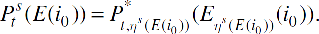
The strategy here is to choose the node with maximum P∗
t,n
(En (i0)) as the transmitting node, that is,

and then by Eq. (28),

Thus, in general, the MSPS-MSSN assumes that the sensor node with higher TSA-MSSN power level has higher “urgency” in transmission.
Based on the TSA-MSSN preprocessing results, MSUS-MSSN chooses the node with the maximal achievable TSA-MSSN utility summation, which is conceptually interpreted as the associated utility functions summation by selecting one node n for transmitting. The specific summation is mathematically defined as, for n = 1…N,

We have,
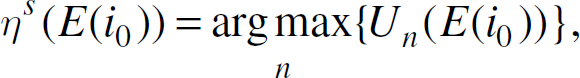
and
To provide an analytical performance comparison between optimal and suboptimal algorithms is difficult. However, we discuss two case studies.
Case 1: TSA-MSSN Active Case: The definition of “active” is that at least one of the N TSA-MSSN power decisions {P∗
t,n
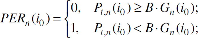
(En (i0)) | n = 1…N} is nonzero. Consider a simplified scenario where “ideal coding” is utilized on every sensor node, and the power control level Pt,n(i0) on the sensor node is continuous. Furthermore, we assume that there is no shadowing uncertainty about the channel, that is holds, instead of Eq. (26) where an uncoded binary information sequence has been assumed. B in Eq. (33) is a constant that depends on the noise power Eq. (34) can be interpreted as follows: For the selected transmitting node n, since According to the simplified model of Eq. (34), the optimal and suboptimal algorithms differ only in the way of choosing the transmission node, η∗ (E(i0)) or η
s
(E(i0)), respectively. Note that under more realistic settings, this claim holds only approximately. When comparing MSPS-MSSN and MSUS-MSSN, we note that the latter takes into considerations both the energy consumption and the number of residual packets on every node, while the former takes into considerations only the transmitting power. A simulation comparison of the optimal and suboptimal algorithms is given in Section V. Case II: TSA-MSSN Sleeping Case: The definition of TSA-MSSN “sleeping” case is that the TSA-MSSN power decision by Eq. (23) is zero for all nodes, that is,
Under this condition, all suboptimal algorithms will keep all nodes sleeping in the current time slot i0. The optimal MTSA-MSSM performs strictly better, since it avoids this restriction by jointly deciding the transmission strategy over all N nodes. Consider the following illustrative example. We set N = 2, and Since virtually all the configurations in nodes/sink fall under the two described cases, one should avoid Case II when employing suboptimal scheduling algorithms. This, however, can be achieved by the special design in the Media Access Control (MAC) layer channel selecting algorithm.


As it has already been mentioned, to avoid the performance degradation in suboptimal algorithms, one should avoid “Case II.” This can be accomplished by running the channel selection algorithm for one specific node n only when it is active, i.e. P∗ t,n (En (i0)) > C. This criterion, on the other hand, also enhances the spectrum efficiency by keeping all the occupied channels busy.
At the current time i0, assume that there are Nall(i0) nodes associated to the mobile sink. And there are M(i0) occupied channels, where obviously M(i0) < Nall(i0). Define a sensor nodes subset A(i0) of {n| n = 1…Nall(i0)} to be,

Then, at time i0, the channel selection algorithm only runs on the newly activated nodes n ∊ Anew(i0), where

Suppose that the maximum number of available channels is Mmax. If M(i0) < Mmax, the channel selecting algorithm can always randomly pick one vacant channel for the new active node, n ∊ Anew(i0). However, if M(i0) = Mmax, the channel selection algorithm selects one of the Mmax occupied channels for the new node, according to some criterion. Although a further discussion on channel selection algorithms is outside the scope of this paper, we give an illustrative example. When M(i0) = Mmax, assume that the system states associated with Mmax channels are Em(i0) (m = 1…Mmax), respectively. Let Am(i0) denote the set of nodes sharing the channel m. We define the overall packets number of channel m, Km(i0), as,

Channel Selecting Algorithm

A simple criterion on deciding the selected channel m∗ for the new node is that Km∗(i0) be minimal. This criterion, however, expresses a rule of thumb, which simply prevents overcrowding any one particular channel. Table 3 describes this algorithm.
The following simulations scenario is considered. The sink is passing through the sensor network region. Some parameters generally comply with IEEE 802.15.4 [6], and are listed in Table 4. The number of transmission power levels is set to 10, and the set of discrete levels is,

λ, which is the parameter to decide the tradeoff between successful transmission and energy consumption, is set to be ‘1’ throughout all the simulations. The setups of the stimulations in Section V-A and V-B, i.e. the nodes/sink locations and the packet numbers, are randomly chosen, satisfying the “active” and ‘sleeping” conditions, respectively. All the results in the figures are the average of 500 Monte-Carlo runs.
We compare the optimal and suboptimal algorithms under “Case I” specified in Section IV-D.1. We assume that two sensor nodes are sharing one specific communication channel, that is N = 2. Without loss of generality, let
Communication Parameters Setup
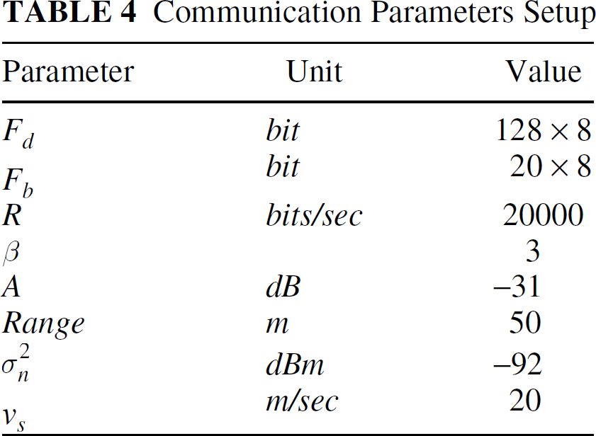
Communication Parameters Setup
Simulations are performed to measure the energy consumption Eall and successful transmission rate Pall of MTSA-MSSN, MSPS-MSSN, and MSUS-MSSN, respectively. In calculating the energy consumption, we omit the RF circuits energy consumption, since it is the same for all algorithms. Then, the definitions of Eall and Pall will be,


respectively, where,

Figures 2 and 3 plot Eall and Pall, respectively, when
The following observations are made: The energy consumption Eall of MSPS-MSSN is much higher than the other two algorithms everywhere; however, it also has a higher Pall than others when
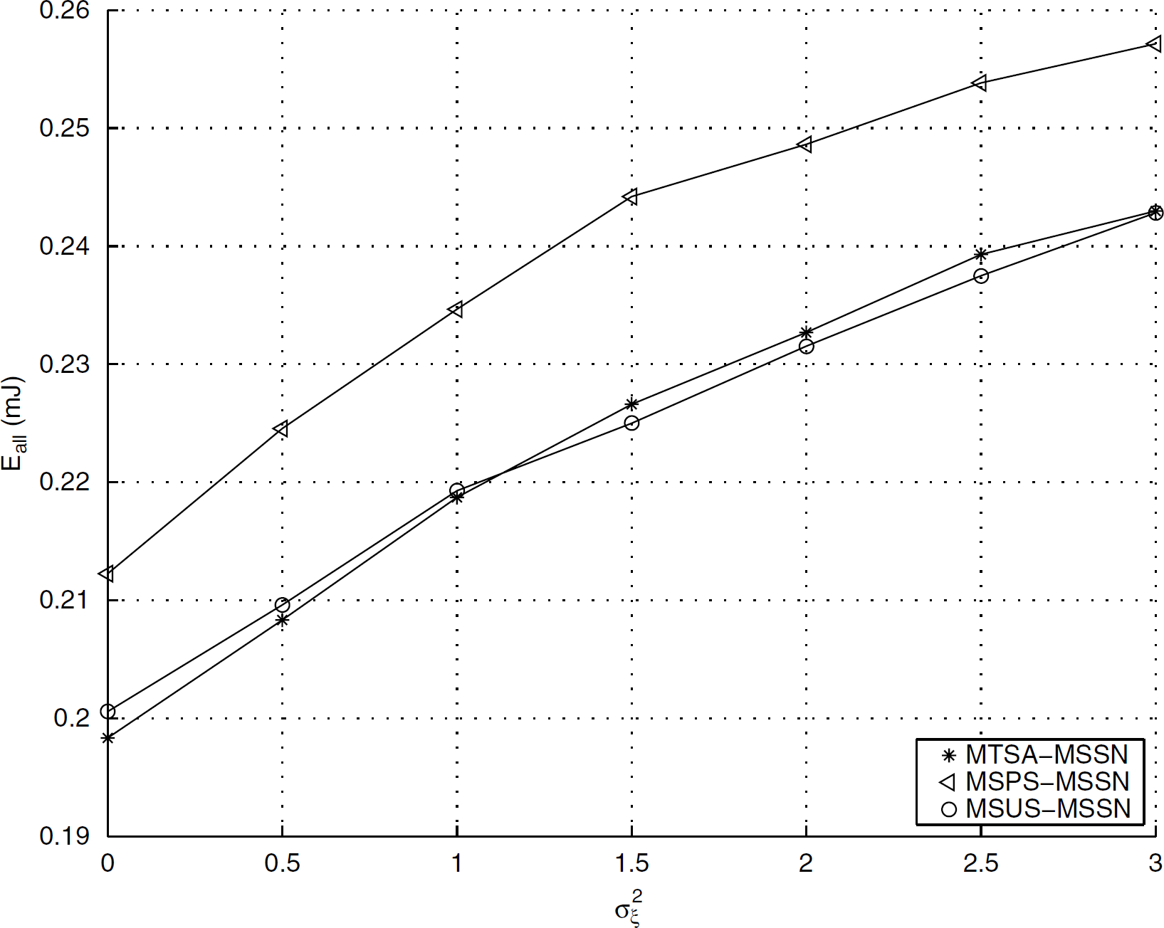
Case I: total energy consumption Eall vs.
We compare Eall and Pall of MTSA-MSSN, MSPS-MSSN, and MSUS-MSSN under “Case II” specified in Section IV-D.2. Again, we assume two sensor nodes are associated with one specific communication channel, which is N = 2. let
Since the number of available time slots are much higher than the number of packets in this simulation, Pall for all the algorithms is 16, which implies that no packet is lost in the transmission. Figure 4 shows the variation of Eall when

Case I: successfully transmitted packets Pall vs.
Centralized vs. Distributed Scheduling
We hereby compare the multiple access MSSN with the SENMA [20], [21]. Although the two have similar network topology, they are nevertheless different types of networks.
In MSSN, we assume certain signal processing capability on individual sensor nodes, which can be viewed as the high level event acquisition [4], instead of raw data acquisition. The sink is dominant in MSSN, since the deterministic scheduling is decided on the sink. SENMA, on the other hand, assumes a simple reachback sensor network, where the sensor nodes transmit raw data to the sink (mobile agent), with no inter-node signal processing. The sink in SENMA, on the other hand, consecutively retrieves the packets from the node with the best channel state. SENMA is a sensor nodes dominant network, because the random access is implemented. SENMA claims low complexity of the sensor nodes. MSSN, however, achieves a higher efficiency and a higher application specific flexibility [1], because of the high level event acquisition. The proposed scheduling algorithms better utilize the higher processing/power capability of the sink, and keep the simplicity of sensor nodes. The choice between MSSN and SENMA should be dependent on the application requirements.
The proposed scheduling algorithms are centralized, since the mobile sink completely decides the transmission strategies. Under the setup of SENMA, [21] proposed the distributed opportunistic scheduling algorithm, by assuming channel state information on sensor nodes. Compared with centralized algorithms, distributed algorithms can save protocol overheads. However, in the multiple access MSSN, since the scheduling criterion is more complicated, we consider that the development of distributed scheduling algorithms for MSSN is not cost-efficient.

Case II: total energy consumption Eall vs.
First, the final state configuration function, given by Eq. (19,27), corresponds to the “Application scenario 1” in [1]. As described in [1], the final state configuration is application specific. Different configurations can be applied with the algorithms proposed in this paper without further difficulty. In both [1] and this paper, we have assumed that the transmission rate R is constant. When this assumption does not hold, and multi-rate channel coding is feasible on sensor node, the strategy space of MTSA-MSSN will be the size of N·Sizeof {Pt}·Sizeof {R}, which corresponds to an increase by a factor of Sizeof {R}, the number of rate control levels. Suboptimal algorithms, such as the MSUS-MSSN, can also be extended to this multi-rate case.
Second, in the channel mode Eq. (3), the small scale multipath fading was not considered. By assuming a small scale fading model, e.g. the Rayleigh fading, in Eq. (3), we need to recalculate the PĚR function in Eq. (12), which is a function of the separating distance D(i), the transmission power level Pt(i), and the transmission rate R. The fading may not be overlooked in some scenarios, especially when the transmission rate is high, and the time diversity over fading states is not achievable. Although multiple receiving antenna diversity can be a solution, another more cost-efficient alternative is the cooperative transmission in a densely deployed sensor network [2]. It utilizes, by the theory of MIMO structure, nodes space diversity instead of receiving antenna diversity. Diverse coding schemes and channel models can be implemented in this framework with non-significant modifications on the scheduling algorithms. The details of the implementations are subject to future research.
Traditionally, packet transmission scheduling is included in the data link layer. However, by exploiting the tradeoff between the successful transmission and the energy consumption, the cross layer design of a consolidate physical and data link layer is needed. In [3], [4], Embedded Wireless Interconnect (EWI) was proposed as the potential universal architecture of wireless sensor networks. EWI is composed of two layers, which are the Wireless Link layer and the System layer, respectively. Under the architecture of EWI, the proposed transmission scheduling algorithms work on the Wireless Link layer of MSSN. It interacts with the upper System layer by the syntax of application information credits, which is then translated into the final state configuration function of the scheduling algorithms.
Conclusion
In this paper, we have studied the operation of MSSN when multiple nodes share one communication channel during the information retrieval. First, we have developed the optimal multinode scheduling algorithm MTSA-MSSN. Since the complexity of MTSA-MSSN increases exponentially with the number of nodes, we propose suboptimal algorithms, which run the single node scheduling algorithm TSA-MSSN individually on every node and then combine the results. The two suboptimal algorithms, MSPS-MSSN and MSUS-MSSN, exhibit the complexity as low as O(N). The performances of optimal and suboptimal algorithms are compared by means of computer simulations. It is shown that the suboptimal algorithms achieve nearly the same performance as the optimal MTSA-MSSN when the channel is “active.”