Sage Journals: Discover world-class research

Abstract

Recent advances in technology have made it possible to build surveillance systems using many low-cost sensor nodes with limited computation and communication capabilities. Due to a potentially large number of nodes deployed, node failures are inevitable and can render a surveillance system that has degraded detection performances. The exposure metric has been proposed earlier to assess the quality of a surveillance system based on the detection performances. In this paper, we characterize the vulnerability of a system in terms of its exposure with respect to the number of faulty nodes and their combinations. Specifically, we assess the exposure of a surveillance network subject to a given number of faulty nodes, and identify the worst-case fault combination for both an idling target and a traversing target. For an idling target, the worst-case fault combination and exposure is analytically identified. For a traversing target, a genetic algorithm based approach is proposed to derive a near worst-case fault combination, and extensive simulation results are presented to show the effectiveness of the algorithm.

Keywords

Sensor Networks Exposure Detection Sensor Deployment Fault Tolerance

I. Introduction

Emerging sensor network technology has enabled the production of a bridge between the computational space and the physical world, using many low-cost sensing devices with limited computation and communication capabilities [1]. Capable of sensing, processing, and communication, the devices (referred to as nodes hereafter) can form a network to collect measurements about the environment and extract useful information in the monitored region. Such sensor networks can be exploited for a variety of purposes. Having been showcased in applications such as wildlife tracking [2, 3] and battlefield intrusion detection [4, 5], one can envision that sensor networks will be an important infrastructure for how we observe the world in the future.

This paper addresses the problem of detecting an intruder or a target in a surveillance sensor network. The surveillance network is comprised of a set of nodes collaborating to detect the presence/absence of a target by exchanging information via wireless communications. Exposure defined as the least probability of detecting a target over all possible target maneuvers has been used to measure the quality of such surveillance networks [4]. Numerous research in literature has focused on the problem of computing the exposure of a given network [4, 6]. However, almost all of them do not consider node failures in the network. This article characterizes the impact of faults and develops algorithms to identify the worst-case fault combinations that make a given network most vulnerable to both idling and traversing targets with and without the presence of obstacles in the region.

The presence of faults mislead the network from arriving at a correct decision and substantially impacts the exposure for the deployment. As exposure varies with different fault combinations, the article identifies the worst-case fault combinations when detecting for either an idling or a traversing target. For an idling target, the article analytically identifies the worst-case fault combination and proposes efficient methods for computing the exposure in the presence of faults and obstacles. For a traversing target, the article proposes a genetic algorithm based approach [7] to find the worst-case fault combination, and compares the exposure in the presence of faults obtained by this approach to that of an exhaustive search. The comparison shows that the genetic algorithm based approach can find the worst-case or near worst-case fault combination with considerable improvement in terms of runtime and exposure.

The remainder of this article is organized as follows. Section II reviews the related work in literature. Section III details the fundamental assumptions and mathematical preliminaries for target detection in sensor networks. Section IV formally defines the problem addressed in this paper. In Section V, the approach to determine the worst-case fault combination(s) for an idling target is presented. In Section VI, a genetic algorithm is developed to search the worst-case fault combination for a traversing target and the evaluation results are presented. The paper concludes in Section VII.

II. Related Work

Exposure and coverage problems of sensor networks have been studied extensively in the literature [4–6, 8–14]. These studies often differ in the exact definition of exposure. In [6], exposure is defined as the integral of signal intensity measured by nodes when a target moves along a path. For a single sensor case, the paper derives the exact shape of the minimum exposure path in a square region. For a multiple sensor case, the paper proposes a centralized approach to determine the minimal exposure path using a high order grid and the shortest path algorithm. In contrast, both [9] and [15] study localized algorithms to identify the minimal exposure path. A probabilistic model of exposure is introduced in [4]. A key aspect of the model is that it considers noise in sensor measurements and directly computes the probability of detecting an idling or a traversing target. Due to noise, the network may incorrectly decide that a target is present when there is actually no target in the region. Trade-offs between exposure and the false alarm probability are also presented in the work. This model has also been used to study sensor deployment strategies to minimize the cost of the deployment subject to an exposure threshold [10]. Moreover, based on the same model, a method to identify the minimal exposure path for targets with varying speeds is proposed in [11].

A number of studies also use sensor network coverage to design sensor deployment strategies. In [16], an integer programming formulation is used to minimize the cost of covering the region of interest. The limitation of the method is that integer programming is not suitable for large sensor network problems. In [12], a heuristic algorithm based on virtual attractive/repulsive forces between nodes is proposed for deploying nodes. The algorithm moves nodes to positions where the virtual forces tend to be balanced. None of the above work considers node failures in the sensor deployment. However, node failures are inevitable in real sensor deployments.

Fusion is a critical issue for making consensus decisions. In the past, a considerable effort has been made to design protocols that reach agreement in the presence of inconsistent faults. For instance, the consensus problem presented in [17] considers n processes with initial values x_i to reach an agreement on a value y = f(x₁ …, x_n), such that each non-faulty process terminates with a value y_i = y. The classic Byzantine general's problem considers one specific node, named “general”, broadcasting its initial value x to all the other nodes, and all non-faulty nodes must terminate with an identical value y = x if the general is non-faulty [18]. To reach a correct agreement in this problem, the system must have at least 3m + 1 nodes, where m is the number of faults. However, fewer studies in literature have focused on fault-tolerance in sensor networks. Motivated by the result in [18], a truncation method is proposed in [5] to deal with inconsistent faults in sensor networks. The paper has given insight into the number of sensors required for obtaining a consistent decision, but are inadequate to assess the worst-case impact of faults on the detection performance. Other work has focused on fault detection and correction [19, 20], or redundancy utilization [21]. Our research addresses the method to identify the worst-case fault combination and the need to evaluate the worst-case detection performance in surveillance networks.

III. Preliminaries

In this section, we describe the fundamental assumptions of the decay model for energy emitted by a target, the impact of obstacles on energy propagation, and the fault model. We then detail the derivation for the probability of detecting a target in a region of interest [4].

A. Energy Model

Consider n nodes randomly deployed in a square field at positions {s₁, s₂ … s_n}, respectively. A target present in the field can be a heat source (such as fire), a vehicle, or a radiological dispersion device (RDD) that can broadcast non-fissile, but highly radioactive particles. The target may constantly be emitting a signal, which can be measured by the nodes. The energy of the target is assumed to decay with distance from the target. Specifically, the target energy measured by node i if the target is at location u is modeled as

E_{i} (u) = {\begin{cases} \frac{α_{i} (u) K}{| u - s_{i} |^{l}} & if | u - s_{i} | > 1 \\ K & otherwise, \end{cases}

(1)

where K is the energy emitted by the target, α_i(u) is the energy distortion factor due to obstacles, |u — s_i| is the Euclidean distance between the node and the target, l is the energy decay coefficient. Depending on the environment, the decay coefficient l is generally between 2.0 to 5.0 [22].

The function α_i(u) characterizes energy distortion caused by obstacles. We use a simplified model for energy distortion as illustrated in Fig. 1. In this model, each obstacle is characterized using two radii, r₁ and r₂, with r₁ ≤ r₂. Given a target, a node, and an obstacle between the target and the node, define t as the perpendicular distance from the center of the obstacle to the line joining the node and the target. Then, the energy distortion factor α is given as

α = {\begin{cases} 0 & t \leq r_{1} \\ \frac{t - r_{1}}{r_{2} - r_{1}} & r_{1} < t < r_{2} \\ 1 & t \geq r_{2} . \end{cases}

FIGURE 1

The model for distortion factor α. PSfrag replacements: 0 < α < 1; α = 0; α = 1; r₁; r₂; t.

Intuitively, the model can be explained as follows. If the node lies between the two tangent lines from the target to the inner circle of radius r₁ then α = 0. If the node lies outside the two tangent lines from the target to the outer circle of radius r₂, then α = 1. If the node lies in the region between the inner and outer tangent lines, then α increases from 0 to 1 with the distance t — r₁ Although the model simply illustrates energy absorbed by round obstacles, it can easily be extended to model other situations such as energy reflection and different shapes of obstacles. In any case, other models that can calculate the target energy strength at a given location can also be used to replace this model without loss of generality.

Measurements of the nodes are inherently corrupted by noise. Let $N_{i}^{2}$ denote the noise energy detected by node i. The total energy detected by node i when a target at position u is $E_{i} (u) + N_{i}^{2}$ .

B. Fault Model

Impacts of faults on detection performance is contingent on both the fusion algorithm and the nodes' fault model. In this article, we cast our analysis over a typical fusion algorithm called value fusion [5], in which nodes periodically report energy measurements to a manager node to arrive at a consensus decision as to the presence or absence of the target. The manager node can be a special node with more powerful computation capability or a workstation in the control facility. We consider the crash fault model in which a faulty node does not send any measured data to the manager node. This fault model is mostly used to characterize mechanical malfunctions, destruction, and energy drainage of sensor nodes.

C. Detection

Based on value fusion, the manager node compares the sum of the energy measurements to a threshold for reaching a consensus. If the sum exceeds the threshold, it decides that there is a target. Otherwise, it decides that there is no target. More specifically, consider a target at a position u in the region. Let E_i denote the target energy measured by node i as described in Eq. (1), and N_i be the noise energy measured by node i. Let $F$ be a set of m nodes. Given the nodes in $F$ are faulty, the probability of detecting a target at position u is

D_{F} (u) = P r o b (\sum_{i \notin F} (E_{i} (u) + N_{i}^{2}) > η)

(2)

= P r o b (\sum_{i \notin F} N_{i}^{2} > - \sum_{i \notin F} E_{i} (u)),

(3)

where η is the threshold for the consensus decision. If the noise that processes at the nodes is independent, then the probability density function of the summation of $N_{i}^{2}$ is the convolution of the probability density function of each individual $N_{i}^{2}$ . In particular, if the noise process N_i is Additive White Gaussian Noise (AWGN) with mean zero and variance one, then $N_{i}^{2}$ is a Chi-Square distribution with one degree of freedom. Since $\sum_{i \notin F} N_{i}^{2}$ can then be obtained by a Chi-Square distribution with n — m degrees of freedom, the probability of detecting a target at position u can be derived as

D_{F} (u) = 1 - F_{χ_{n - m}^{2}} (η - \sum_{i \notin F} E_{i} (u)),

(4)

where $F_{χ_{n - m}^{2}}$ (x)3 is the cumulative distribution function of Chi-square with n — m degrees of freedom. Due to the noise, the consensus decision may incorrectly decide that a target is present while there is no target in the region. Thus, the false alarm probability can be computed by

F A = P r o b (\sum_{i \notin F} N_{i} > η) .

Given a tolerable false alarm probability, one can determine the corresponding η. In general, detection probability and false alarm probability are closely related. A higher detection probability always comes with a higher false alarm probability.

D. Exposure

1) Idling target

Let I be a period of observation and nodes detect the target energy in a periodic manner every T time units. Without loss of generality, we assume I is divisible by T. Let $F$ be a set of m nodes. Given the nodes in $F$ are faulty, the probability of detecting a target at u in a period of observation I can be expressed as

P_{F} (u) = 1 - (1 - D_{F} (u))^{1 / T}, 3

(5)

where $D_{F} (u)$ is the probability of detecting a target at u when the nodes in (are faulty as given in Eq. (2). Exposure for an idling target is defined as the least probability of detecting the target over all possible fault combinations and target positions during the period I. To facilitate the calculation, the monitored region is divided into a grid. The granularity of the grid trades off computational load with accuracy of target positions. The target is assumed to be able to appear at any grid point in the region. Formally, exposure for an idling target is defined as

ε = min_{F \subseteq C_{m}} (min_{u \in G} P_{F} (u)),

(6)

where C_m is the set of all possible combinations of m faults and G is the set of all grid points within the monitored region. The corresponding target position for exposure is called the exposure point.

2) Traversing target

For evaluating the exposure for a traversing target, the region is also divided into a grid. The target is assumed to traverse from the left to the right periphery along a path P consisting of edges between adjacent grid points. Assume that the target is not detected if and only if it is not detected at any point on the path. Let G(P) denote the probability that a target is not detected along the path P and $F$ is the set of m faults. Then, G(P) is given by

G (P) = \prod_{e \in P} (1 - D_{F} (e)),

(7)

where e is a grid edge and $D_{F} (e)$ is the probability of detecting the target on the grid edge e when the nodes in $F$ are faulty. To calculate $D_{F} (e)$ , one approximation is to take the target energy measurement of each node when the target is in the center of grid edge e and then plug in Eq. (2). Another approximation is to use the average target energy measurement of each node when the target traverses across grid edge e. The exposure for a traversing target in the region can be derived as

ε = min_{F \subseteq C_{m}} min_{P \subseteq P} (1 - G (P)),

∗

where ℙ is the set of all possible target paths. The corresponding path for exposure is called exposure path.

If the set of m faulty nodes is fixed, we can find the exposure path on a graph as follows. Given m faulty nodes, assign a weight $w_{e} = | \log (1 - D_{F} (e)) |$ to each grid edge. Note that D_F(e) is between 0 and 1, so the log term is negative. From Eq. (7),

| \log G (P) | = | \sum_{e \in P} \log (1 - D_{F} (e)) | = \sum_{e \in P} w_{e} .

(8)

To find the exposure is to maximize G(P), which is equivalent to finding the minimal sum of weights on the potential path P. Further, the minimal sum of weights can be determined by the shortest path from the left periphery to the right periphery. To find the shortest path, create a fictitious source point p_s and a fictitious destination point p_d. Connect p_s to all the grid points on the left periphery and p_d to those on the right periphery with zero weight. Find the shortest path from p_s to p_d. Denote W as the weight on the shortest path P∗. We have W = |log G(P∗)| and the exposure is

ε = 1 - 10^{- W} .

Figure 2 shows a procedure to find the exposure path.

FIGURE 2

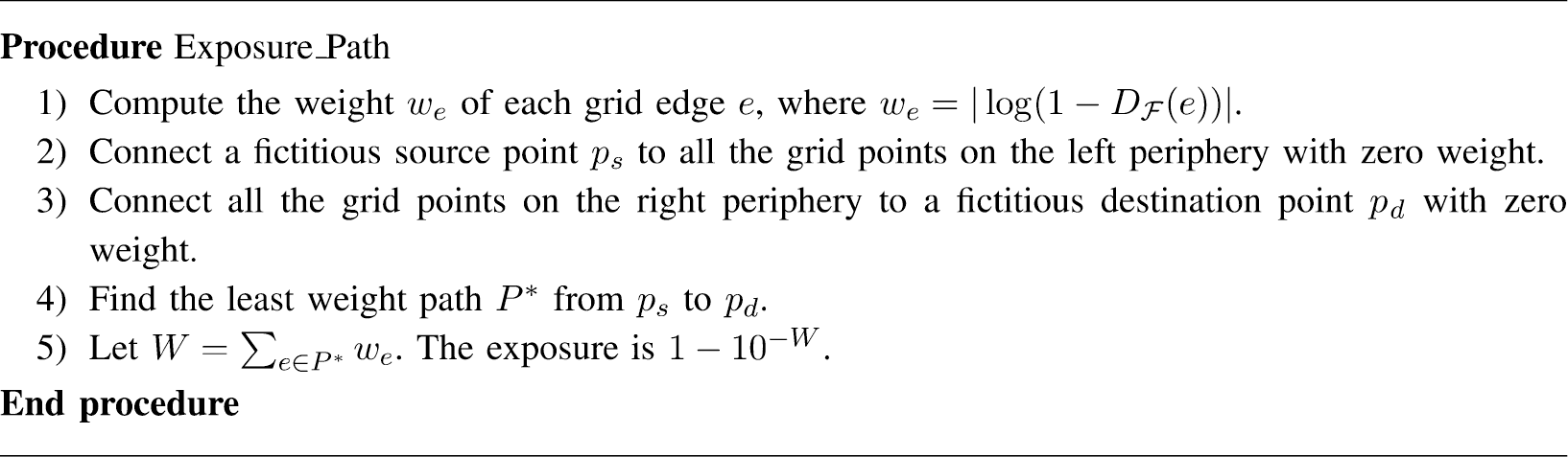
The pseudo-code for searching the exposure path.

IV. Problem Formulation

As nodes can fail at a certain rate during operation, detection performance of a surveillance sensor network needs to be evaluated as a function of time. A commonly used relationship between failure rate and time is the bathtub curve [23]. A similar model may apply for sensors deployed in a region. Indeed, a realistic failure rate function should assume high failure rate during deployment, then low failure rate for a certain period, and high failure rate again for possibly running out of battery. With nodes failing over time, the system is said to be operational if its exposure is above a desired threshold e_d. For system maintenance, it is useful to know the probability that a system is operational at a given time t. The probability can be derived as

P (t) = \sum_{m = 0}^{n} \sum_{F \subseteq C_{m}} P_{f} (F, t) P_{n} (F, t) I (F, e_{d}),

(9)

where C_m is the set of all combinations of m faults, $P_{f} (F, t)$ is the probability that nodes in $F$ are faulty, $P_{f} (F, t)$ is the probability that the remaining nodes are non-faulty, and $P_{n} (F, t)$ is a function indicating if the system is operational in case nodes in $F$ are faulty. $I (F, e_{d}) = 1$ if the exposure when nodes in $F$ are faulty is above e_d. Otherwise, $I (F, e_{d}) = 0$ . In particular, if all the nodes have the same failure rate function, $P_{f} (F, t)$ and $P_{n} (F, t)$ are given by

\begin{aligned} P_{f} (F, t) = ρ (t)^{| F |} \\ P_{n} (F, t) = (1 - ρ (t))^{n - | F |}, \end{aligned}

where ρ(t) is the probability that a node is faulty at time $| F |$ is the cardinality of $F$ . However, to compute Eq. (9) requires determining the function $I (F, e_{d})$ for all the combinations of possible faults in $F$ , i.e., 2ⁿ combinations if n nodes are deployed. Instead, a lower bound of Eq. (9) can be obtained by

P (t) \geq \sum_{m = 0}^{n} (\binom{n}{m}) ρ (t)^{m} (1 - ρ (t))^{(n - m)} I (m, e_{d}),

(10)

where I(m, e_d) is a function indicating if the system is operational in the worst-case scenario when m nodes are faulty. I(m, e_d) = 1 if the worst-case exposure when m nodes are faulty is above e_d. Otherwise I(m, e_d) = 0.

In order to calculate Eq. (10), the worst-case fault combination with m faulty nodes and the worst-case exposure need to be determined. Specifically, the problem can be formulated as follows. Given n nodes deployed in a region to detect unauthorized targets. If m out of the n nodes are faulty, determine the worst-case combination of m faulty nodes that gives the least exposure. As the number of nodes is potentially large, it is impractical to find the worst-case fault combination by exhaustive search. Instead, efficient algorithms are required to identify the worst-case fault combinations for both idling and traversing targets in the monitored region.

V. Idling target

A. Worst-case Fault Combination

Consider a sensor network with total n nodes and m of the nodes are faulty. Assume that the noise process is AWGN with mean zero and variance one. A direct computation of the exposure for idling targets using Eq. (6) requires one to calculate the detection probability for all possible combinations of m faults. However, it is impractical to check all of the $(\binom{n}{m})$ fault combinations as n grows large. As a result, the worst-case fault combination is analyzed to develop efficient search algorithms for both cases of a region with and without the presence of obstacles.

1) No obstacles

Consider the expression of detection probability in Eq. (4). Since $F_{X_{n - m}^{2}} (x)$ is a non-decreasing function of x, we have that $D_{F} (u)$ is a non-decreasing function of E_i(u), which is the energy reading reported by node i. Thus, a node that reports higher energy readings would have more significant impact on the detection probability. In other words, for a target at a position u, since the energy emitted by the target decreases with distance, the closer the faulty nodes are to the point u, the more the detection probability would drop. This intuitive result is formally stated in Theorem 1 and is used to develop an efficient search algorithm for the worst-case fault combination.

Theorem 1

Let P_m(u) be the probability of detecting a target at position u in a decision period when the m nodes closest to position u are faulty. The exposure is the minimum P_m(u) over all possible target positions u, i.e.,

ε = min_{F \subseteq C_{m}} (min_{u \in G} P_{F} (u)) = min_{u \in G} P_{m} (u) .

Proof

Since the numbers of fault combinations and the grid points are finite, we have

ε = min_{F \subseteq C_{m}} min_{u \in G} P_{F} (u) = min_{u \in G} min_{F \subseteq C_{m}} P_{F} (u) .

(11)

We first prove that P_m(u) is the minimum probability of detecting a target at u over all possible fault combinations. That is

P_{m} (u) = min_{F \subseteq C_{m}} P_{F} (u) .

(12)

From the relation between Eq. (2) and Eq. (5), $P_{F} (u)$ is an increasing function of $D_{F} (u)$ is a non-decreasing function of $\sum_{i \notin F} E_{i} (u)$ . Clearly, $P_{F} (u)$ is minimized when the sum of energy $\sum_{i \notin F} E_{i} (u)$ is minimal for a given target position u. Since the closer a node to u, the higher its reading, $\sum_{i \notin F}^{i \notin F} E_{i} (u)$ is minimal when the m closest nodes are faulty. Thus, Eq. (12) holds and the theorem then follows from Eq. (11) and Eq. (12).

The algorithm of finding the worst-case fault combination examines all of the grid points in the region, i.e., all possible target positions. For each grid point u, assume that the m closest nodes to u are faulty. Compute the probability of detecting a target at u using Eq. (5). The minimal detection probability over all the grid points is guaranteed to be the exposure as stated in Theorem 1, and the corresponding set of faulty nodes is the worst-case fault combination. Figure 3 lists the procedure to calculate the exposure for an idling target without obstacles.

FIGURE 3

Algorithm for calculating the exposure for an idling target with obstacles.

Note that exhaustive search for the worst-case fault combination has complexity of order $(\binom{n}{m})$ For this algorithm, the complexity depends on the number of grid points.

2) Obstacles

Obstacles, such as buildings or trees, are commonly present in the field. We now extend the method to find the worst-case fault combination in the presence of obstacles. Similarly, the goal is to identify the nodes that have the most significant impact on the detection probability. Since energy propagation is distorted by obstacles, we cannot just use distance from the target position to justify how much the node can contribute to the sum of target energy $\sum_{i \notin F} E_{i} (u)$ However, it is still possible to identify the nodes with higher contribution by sorting the target energy E_i(u). A similar algorithm can be developed as shown in Fig. 4. The idea of the algorithm is as follows. For each grid point (target position) u, calculate the target energy detected by each node, i.e., E_i(u). Assume that the m nodes with the highest energy readings are faulty. Compute the probability of detecting a target at u. The minimal detection probability over all of the grid points is guaranteed to be the exposure. The method is proved in Theorem 2.

FIGURE 4

Algorithm for calculating the exposure for an idling target with obstacles.

Theorem 2

Let H be the set of the m nodes with the highest energy readings for a target at u with the presence of obstacles and P_H(u) be the probability of detecting the target in a decision period when the nodes in H are faulty. The exposure is the minimum P_H(u) over all possible target position u, i.e.,

ε = min_{u \in G} P_{H} (u) .

Proof

Since the numbers of the fault combinations and the grid points are finite, we have

ε = min_{F \subseteq C_{m}} min_{u \in G} P_{F} (u) = min_{u \in G} min_{F \subseteq C_{m}} P_{F} (u) .

Now we prove that P_H(u) is the minimum probability of detecting a target at u over all possible fault combinations in the presence of obstacles, i.e.,

P_{H} (u) = min_{F \subseteq C_{m}} P_{F} (u) .

(13)

From Eq. (2) and Eq. (5), P_F(u) is an increasing function of $\sum_{i \notin F} E_{i} (u)$ . Therefore, $P_{F} (u)$ is minimized when $\sum_{i \notin F} E_{i} (u)$ is minimal, which occurs when the m nodes in H are faulty. Thus, Eq. (13) holds and the theorem then follows.

In the presence of obstacles, the algorithm uses the energy detected by each node to find the worst-case fault combination rather than the distance from the target to the node.

Indeed, the case with the absence of obstacle is a special case of this algorithm. However, using the distance to determine the worst-case fault combination as shown in Fig. 3 is simpler for the cases without the presence of obstacles. The extra work in the presence of obstacles is to calculate the energy distortion factor. The complexity of the algorithm still depends on the number of grid points.

B. Simulations

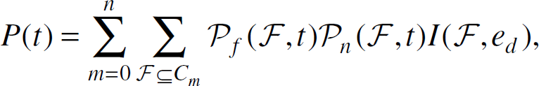
In the first simulation, we illustrate the profile of the probability of detecting an idling target in a 20 × 20 region. In order to cover the monitored region well, nodes are deployed in a 26 × 26 region. We randomly deploy 50 nodes in the enlarged region. An idling target is assumed to emit energy with K = 50 and may appear on any point (x, y) with x, y = 1, 2, …, 20. Noise is assumed to be AWGN with mean zero and variance one. The threshold η is chosen such that the false alarm probability of each detection attempt is 0.001. The manager node makes a detection decision for every 30 attempts of energy measurements. Figure 5(a) shows the profile of detection probability in the region without the presence of faulty nodes. The darker the region the lower the detection probability. The exposure point is located in (12, 0), which is relatively far from the nodes in the vicinity and is the darkest spot in the region. Figure 5(b) shows the profile of detection probability for the same deployment with the presence of three faulty nodes. The exposure point is found by the algorithm shown in Fig. 3. The exposure point moves to (14, 0). From the figure, it is clear that the position (14, 0) is the furthest point from the vicinity nodes if the closest three nodes at (16.05, −0.82), (16.79, 0.94), and (18.25, 2.33) are failed. Thus, the probability of detecting a target at (14, 0) can drop lower than that at (12, 0). In addition, the exposure drops from 0.86 to 0.53 with the presence of three faults.

FIGURE 5

The profile of detection probability in the absence of obstacles. (a) No faults; (b) Three faults.

In the second simulation, five obstacles are placed randomly in the region. The radii r₁ and r₂ of the obstacles are 1 and 2 respectively. The other parameters are the same as those in the previous simulation. Figure 6(a) and 6(b) illustrate the profiles of detection probability without and with three faulty nodes respectively. With the presence of obstacles, the energy distortion must be calculated when applying the algorithm in Fig. 4 to determine the exposure point. From the figures, the exposure point is dramatically moved from (3, 10) to (4, 6) with the presence of faults. Obviously, point (4, 6) becomes a great position for the target to hide if the nodes at (2.91, 6.11), (1.19, 6.19), and (3.9, 2.21) are faulty. Moreover, the exposure drops dramatically from 0.67 to 0.13 in the presence of faults and obstacles.

FIGURE 6

The profile of detection probability in the presence of five obstacles. (a) No faults (b) Three faults.

Figure 7 shows the average impact of faults and obstacles on exposure. Each bar in the figure is an average of exposure over 100 deployments with 50 nodes. Nodes and obstacles are placed randomly and the simulation parameters are the same as the previous simulations. It is noted that η is independent of the number of obstacles but depends on the number of nodes participating in the fusion. Therefore, η must be adjusted for a different number of faulty nodes such that the comparison is based on a fixed false alarm probability. As expected, the exposure decreases with the number of faulty nodes and obstacles. On average, exposure tends to drop faster with the number of faults than the number of obstacles. However, the size, location, and the characteristic radii r₁ and r₂ can have different impact on the exposure.

FIGURE 7

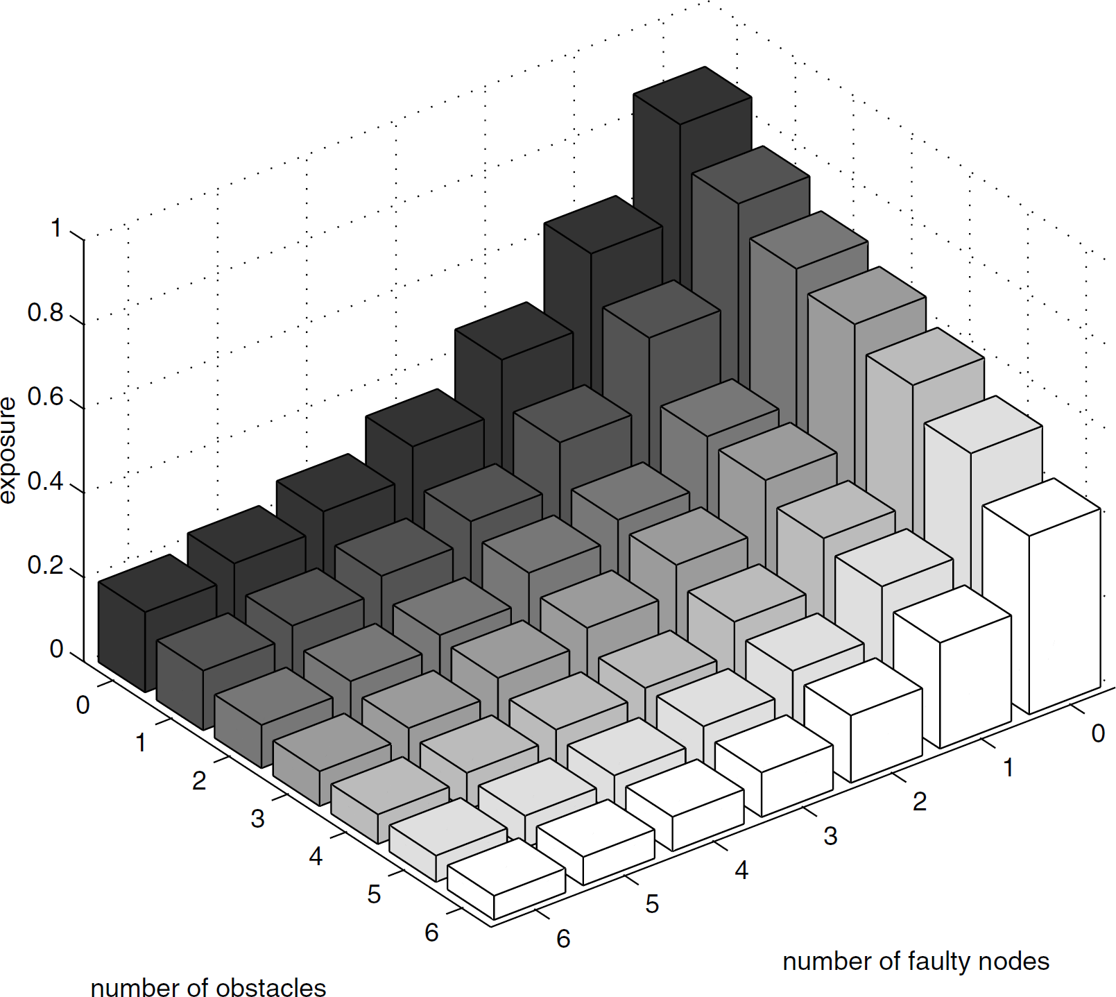
Average exposure vs number of faulty nodes and obstacles.

VI. Traversing Target

A. Worst-case Fault Combination

For target traversal, the target is assumed to move across the region from the left periphery to the right periphery with constant speed. Exposure for a traversing target is not merely a function of the distance from the target to the nodes, but associated with a series of target positions. Consequently, it is not sufficient to find the combination of faults that makes a single point poorly exposed as in the idling target case. Instead, a fault combination that makes a series of grid points hard to detect simultaneously has to be found. A first intuition for the worst-case fault combination may be the m closest nodes to the exposure path in the absence of faults. Unfortunately, this is not always the case. The exposure path in the presence of faults can be far away from the exposure path in the absence of faults.

The proposed solution is a genetic algorithm based approach that does not guarantee finding the worst-case fault combination, but has been found to be effective in a high percentage of the simulated examples. The premise of the algorithm is based on the observation that a combination of faults that intersects with the worst-case fault combination often gives lower exposure than a combination of faults that does not intersect with the worst-case fault combination. The algorithm is designed so that combinations of faults that intersect with the worst-case fault combination have a chance to be coupled to produce the worst-case fault combination.

Figure 8 lists the procedure of the genetic algorithm based approach. Initially, the algorithm randomly generates a population of N chromosomes. A chromosome is a fault combination with m distinct nodes. Each chromosome is assigned a fitness value, which is defined as (1 − ϕ) where $φ = min_{P \subseteq P} (1 - G (P))$ is the minimal detection probability when the nodes in the chromosome are faulty. In other words, the goal of the algorithm is to find a chromosome with the highest fitness value. The algorithm is an iterative method with the following steps.

Selection: Selects two chromosomes with probability proportional to the fitness values such that fault combinations with low φ can be selected with high probability.

Crossover: The genes (i.e., faulty nodes) in the two selected chromosomes are rotated for a random distance in position. Then, the two chromosomes generate two children by exchanging genes pair by pair with probability p_cross. The best two chromosomes with the highest fitness values of the four chromosomes (two parents and two children) are kept in the population.

Mutation: Through mutation, the algorithm can further diversify the population. The algorithm randomly picks one chromosome from the population and changes each gene in the chromosome with a very small probability p_mul.

FIGURE 8

Genetic algorith for searching the least exposure path.

A copy of the overall best chromosome is recorded and the above three steps are repeated until the stopping criterion is satisfied. Possible stopping criteria include:

Stop after a specified number of fitness evaluations;

Stop when the best chromosome does not change for a period of time;

Stop after a specified runtime.

The algorithm is executed once at the control center after the nodes are deployed to diagnose the weakness of the surveillance system. Therefore, the genetic algorithm would not affect the operation of the detection.

B. Simulations

We compare the fault combination found by the genetic algorithm based approach to the true worst-case fault combination found by exhaustive search. The parameters for the genetic algorithm based approach in all the following simulations are shown in Table 1 unless specified otherwise. The target is assumed to traverse across the monitored region from left to right periphery. The noise process is AWGN with mean zero and variance one. The stopping criterion used in the genetic algorithm is to stop after 10, 000 fitness evaluations. In the first simulation, we observe 100 deployments for both cases with and without obstacles in the region. In each deployment, 50 nodes are randomly placed in the deployed region. For the cases with the presence of obstacles, five obstacles are randomly placed in the deployed region. We assume that six out of the fifty nodes are faulty and use the genetic algorithm based approach to find a near worst-case fault combination and the exhaustive search to find the true worst-case fault combination.

TABLE 1
Simulation parameters

Population size C 100

Crossover probability p_cross 0.5

Mutation probability p_mut 0.001

Number of fitness evaluations 10,000

Power emitted by the target 30

False alarm probability 0.001

Obstacle radius r₁ 1

Obstacle radius r₂ 2

Monitored region size 20 × 20

Deployed region size 26 × 26

Figure 9(a) shows the percentage of deployments in which the genetic algorithm found the optimal solution (the worst-case fault combination) during the execution. After 10, 000 fitness evaluations, the algorithm found the worst-case fault combinations in 80% of the deployments without the presence of obstacles, and in 72% of the deployments with the presence of obstacles. Furthermore, in most of the deployments, the worst-case fault combination was found within 3000 fitness evaluations. Comparing with the total 15, 890, 700 fault combinations, this is only 0.02% of the total number. This shows that the genetic algorithm can save a considerable amount of time in a large network where doing exhaustive search is impractical. In fact, for a deployment with 50 nodes, it takes about two hours to exhaustively search the worst-case fault combination with six faulty nodes on a Pentium 2.5GHz Linux machine with 1GB memory. In contrast, the genetic algorithm takes about one minute for 10, 000 fitness evaluations and finds a relatively good solution.

FIGURE 9

Comparison of the genetic algorithm and exhaustive search. (a) The fraction reaching optimal solution. (b) The average difference of exposure from optimal.

Figure 9(b) shows the average difference between the true exposure and the exposure obtained by the genetic algorithm if the worst-case fault combination is not found. Although the genetic algorithm does not guarantee to find the optimal solution, the deviation from the true exposure is not very large at the end of the execution. With and without the presence of obstacles, the average deviation is about 0.17. Note that this is only for the deployments that the worst-case fault combinations were not found and those were only 20% and 28% of the deployments in the cases without and with the presence of obstacles, respectively.

Figure 10(a) compares the average exposure obtained by the genetic algorithm based approach to a random search method without the presence of obstacles. The random search method iteratively chooses an arbitrary combination of six faulty nodes and calculates the exposure with faults for the deployment. For fair comparison, it also runs 10, 000 iterations and keeps the best solution until the end of execution. Each data point in the figure is also an average over 100 deployments. We also investigated deployments with 25, 50, and 75 nodes and assumed six of the nodes are faulty. The results are slightly different in each case and are shown in Fig. 10. For 75 nodes, exposure is high since the node density is high. Six faulty nodes is a relatively small number and is likely to have very little impact on the overall exposure no matter what fault combination is chosen. On the other hand, for 25 nodes, the exposure is already very low and there is no significant change in the exposure no matter what fault combination is chosen. In contrast, for 50 nodes, the number of nodes and the monitored region size is in some sense in a critical point such that the positions of faulty nodes can affect exposure dramatically. From the result, the genetic algorithm based approach can approach the optimal solution very quickly. Furthermore, in all three cases, the genetic algorithm based approach can find better solutions than the random search method. The results for the cases with five obstacles randomly placed in the region are shown in Fig. 10(b). Similar results are shown as in Fig. 10(a), except the exposure is lower because of the presence of obstacles in the region.

FIGURE 10

Comparison of the genetic algorithm and random search. (a) Without obstacles (b) With obstacles.

In Fig. 11, we investigate the impact of the number of faulty nodes on the genetic algorithm based approach. We choose the typical scenario of deploying 50 nodes randomly in each deployment and plot the average exposure over 100 deployments. In such scenarios, exposure is more sensitive to the number of faults. As expected, exposure is lower as more nodes become faulty. However, the genetic algorithm based approach still converges very fast within 3000 fitness evaluations for all the cases. Note that the total number of fault combinations is $(\binom{n}{m})$ where n is the number of nodes and m is the number of faulty nodes. Similar results are also seen in the simulations with the presence of five obstacles as shown in Fig. 11(b).

FIGURE 11

The convergence of the genetic algorithm for different number of faults. (a) Without obstacles (b) With obstacles.

Figure 12 shows the results of the genetic algorithm based approach with different number of obstacles. The results are also the average over 100 deployments with 50 nodes randomly deployed in the region and six of the nodes are assumed to be faulty. The figure shows that the exposure with ten obstacles is higher than that with five obstacles. This is because when there are a lot of obstacles in the region, a large number of paths are blocked by the obstacles. Hence, the target is easier to be detected. In contrast, if there are only a few number of obstacles, the target still has many paths to choose and the energy absorbed by obstacles makes the target harder to be detected. However, the genetic algorithm based approach still converges very fast and performs well with a different number of obstacles.

FIGURE 12

The convergence of the genetic algorithm for different number of obstacles.

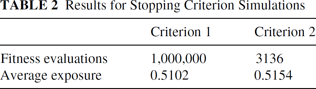
Different stopping criteria for the genetic algorithm are also examined to compare the run time and the best solution found by the genetic algorithm. The simulation parameters are the same as those in Table 1, except 150 nodes are placed in the region and the energy emitted by the target is reduced to 10. The first stopping criterion is to stop after one million fitness evaluations. We made the number large to ensure that the algorithm reaches a good solution. The second stopping criterion is to stop when the number of fitness evaluations exceeds 3000 and the best solution does not change for a period of time, which is chosen as 10% of the current number of fitness evaluations. The results are given in Table 2. The final exposure values of the two stopping criteria are almost the same, while the stopping criterion 2 needs much less number of fitness evaluations. Thus, even with a large number of nodes deployed, the genetic algorithm can stil stop very early and find a good solution using stopping criterion 2.

TABLE 2

Results for Stopping Criterion Simulations

	Criterion 1	Criterion 2
Fitness evaluations	1,000,000	3136
Average exposure	0.5102	0.5154

VII. Conclusion

This paper characterizes the vulnerability of sensor networks to faults. The exposure metric for unauthorized target idling and target traversal is used to measure the quality of the deployment. Determining the worst-case fault combination is a critical issue for evaluating exposure in the presence of faults. In this paper, the worst-case fault combination for an idling target is analytically characterized and algorithms are presented to efficiently identify the worst-case fault combination with and without obstacles in the monitored region. For a traversing target, a genetic algorithm based approach is proposed to search the worst-case fault combination. Simulation results show that the genetic algorithm can find the worst-case fault combination in most cases and the convergence of the algorithm to the optimal solution is very fast in various deployment conditions. This work provides an assessable metric to evaluate the robustness of surveillance systems in the presence of faults for different target activities. Since faults are inevitable in real systems, we believe that this evaluation is important in actual sensor deployments and must be considered when deploying the nodes.

References

Estrin

Girod

Pottie

, and Srivastava

, “Instrumenting the World With Wireless sensor Networks,” in Proc. of the International conference on Acoustics, Speech, and Signal Processing (ICASSP 2001) 4, pp. 2033–2036, 2001.

Mainwaring

Polastre

Szewezyk

Culler

, and Anderson

, “Wireless Sensor Networks for Habitat Monitoring,” in ACM International Workshop on Wireless Sensor Networks and Applications (WSNA '02), Atlanta, GA, pp. 88–97 Sept. 2002.

Juang

Oki

Wang

Martonos

Pch

, and Rubenstein

, “Energy-efficient Computing for Wildlife Tracking: Design Tradeoffs and Early Experiences with Zebranet,” in ASPLOS, San Jose, CA, pp. 96–107, Oct. 2002.

Phipatanasuphorn

, and Ramanathan

, “Vulnerability of Sensor Networks to Unauthorized Traversal and Monitoring,” IEEE Transactions on Computers, 53, 3, pp. 364–369, Mar. 2004.

Clouqueur

Saluja

K. K.

, and Ramanathan

, “Fault-tolerance in Collaborative Sensor Networks for Target Detection,” IEEE Transactions on Computers, 53, 3, pp. 320–333, Mar. 2004.

Meguerdichian

Koushanfar

, and Potkonjak

, “Exposure in Wireless Ad-hoc Sensor Networks,” in MOBICOM, Rome, Italy, pp. 139–150, July 2001.

Goldberg

D. E.

, Genetic Algorithms in Search, Optimization, and Machine Learning, Reading, MA: Addison-Wesley, 1989.

Meguerdichian

Koushanfar

Potkonjak

, and Srivastava

M. B.

, “Coverage Problems in Wireless Ad-hoc Sensor Networks,” in INFOCOM, pp. 1380–1387, Apr. 2001.

Meguerdichian

Slijepcevic

Karayan

, and Potkonjak

, “Localized Algorithms in Wireless Ad-hoc Networks: Location Discovery and Sensor Exposure,” in MOBIHOC, pp. 106–116, Oct. 2001.

10.

Clouqueur

Phipatanasuphorn

Ramanathan

, and Saluja

K. K.

, “Sensor Deployment Strategy for Detection of Targets Traversing a Region,” Journal on Mobile Networks and Applications, 8, 453–461, Aug. 2003.

11.

Clouqueur

Ramanathan

, and Saluja

K. K.

, “Exposure of Variable Speed Targets through a Sensor Field,” in Proc. of the 6th Ann. Conf. on Information Fusion, 1, pp. 599–605, July 2003.

12.

Zou

, and Chakrabarty

, “Sensor Deployment and Target Localization based on Virtual Forces,” in INFOCOM, 2, pp. 1293–1303, Apr. 2003.

13.

Dhillon

S. S.

, and Chakrabarty

, “Sensor Placement for Effective Coverage and Surveillance in Distributed Sensor Networks,” in Proc. IEEE Wireless Communications and Networking Conference, 3, pp. 1609–1614, Mar. 2003.

14.

Wong

Y.-H.

, and Sayeed

, “Detection, Classification, and Tracking of Targets,” IEEE Signal Processing Magazine, 19, 2, pp. 17–19, Mar. 2002.

15.

Veltri

Huang

, and Potkonjak

, “Minimal and Maximal Exposure Path Algorithms for Wireless Embedded Sensor Networks,” in Proceedings of the First International conference on Embedded Networked Sensor Systems, Los Angeles, CA, pp. 40–48, Nov. 2003.

16.

Chakrabarty

Iyengar

S. S.

, and Cho

, “Grid Coverage for Surveillance and Target Location in Distributed Sensor Networks,” IEEE Transactions on Computers, 51, pp. 1448–1453, Dec. 2002.

17.

Barborak

Malck

, and Dahbura

, “The Consensus Problem in Fault-tolerant Computing,” ACM Computing Surveys, 25, 2, pp. 171–220, June 1993.

18.

Lamport

Shostak

, and Pease

, “The Byzantine Generals Problem,” ACM Transactions on Programming Languages and Systems, 4, 3, pp. 382–401, July 1982.

19.

Krishnamachari

, and Iyengar

S. S.

, “Distributed Bayesian Algorithms for Fault-tolerant Event Region Detection in Wireless Sensor Networks,” IEEE Trans. Comput., 53, 3, pp. 241–250, 2004.

20.

Chessa

, and Santi

, “Crash Faults Identification in Wireless Sensor Networks,” Computer Communications, 25, 14, pp. 1273–1282, 2002.

21.

Zou

, and Chakrabarty

, “Fault-tolerant Self-organization In Sensor Networks,” in DCOSS, pp. 191–205, June 2005.

22.

Hata

, “Empirical Formula for Propagation Loss in Land Mobile Radio Service,” IEEE Transactions on Vehicular Technology, 29, pp. 317–325, Aug. 1980.

23.

Pradhan

, Fault-tolerant Computer System Design. Prentice Hall, 1995.

Population size C	100
Crossover probability p_cross	0.5
Mutation probability p_mut	0.001
Number of fitness evaluations	10,000
Power emitted by the target	30
False alarm probability	0.001
Obstacle radius r₁	1
Obstacle radius r₂	2
Monitored region size	20 × 20
Deployed region size	26 × 26

Vulnerability of Surveillance Networks to Faults

Abstract

Keywords

I. Introduction

II. Related Work

III. Preliminaries

A. Energy Model

C. Detection

1) Idling target

A. Worst-case Fault Combination

1) No obstacles

Theorem 1

Proof

Theorem 2

Proof

A. Worst-case Fault Combination

References