Sage Journals: Discover world-class research

Abstract

One key issue in designing battery-powered wireless sensor networks is to properly control the energy consumption of the sensor nodes in order to prolong their operation time (i.e. lifetime). In this article, we present a real-life application of wireless sensor networks in trains to monitor the goods conditions in a long-distance transportation. We study the wireless sensor network deployment problem in developing a monitoring system with the goal of maximizing the network lifetime under constraints derived from the real application scenario. The key technical problem to solve is to determine the sensor placement and the transmission level for each sensor node, as well as the appropriate number of sensor nodes. We first formulate the problem with a realistic discrete power model as a mixed integer linear programming problem. Then, a two-step efficient deployment heuristic is proposed to satisfy these constraints step by step. The evaluation results indicate that the proposed heuristic performs almost the same as the optimal mixed integer linear programming solution. Moreover, the wireless sensor network with appropriate number of nodes can improve its lifetime up to 10.6% for a train with 80 boxcars. We also discussed a tested experiment in a laboratory environment, as well as the real implementation of the whole monitoring system.

Keywords

Wireless sensor networks sensor deployment lifetime maximization

Introduction

In recent years, wireless sensor networks (WSNs) have been integrated into many real-life applications, such as habitat study,¹ environment/ecology monitoring,² railway bridge monitoring,³ datacenter monitoring,⁴ and industrial monitoring.⁵ A WSN is generally composed of tens to thousands of sensor nodes, each of which is equipped with several sensing devices, a short-range wireless transceiver, a low-cost computational capacity processor, and a limited battery-supplied energy. Sensor nodes monitor some surrounding environment and forward data obtained to a base station, which collects data and then transmits this data to a remote control center.

Although much attention has been paid to designing sensors for low power consumption, sensor nodes still have very limited operation lifetime. Moreover, it may be infeasible or expensive to replace the batteries in sensor nodes after deploying a WSN. One critical and challenging problem in WSNs is how to manage their energy consumption to achieve the maximum lifetime under the battery energy constraint.

In general, multi-hop data forwarding schemes,⁶ where the data of sensor nodes that are far away are relayed by their neighbor nodes that are closer to the base station, are more energy efficient than direct transmission when the cover range is fairly large. However, a WSN may still survive only a very limited lifetime if adopting no effective policy to deal with the increased transmission activities of such near-by sensor nodes which depletes the battery energy quickly.⁷ To address this problem, one can place more sensor nodes close to the base station and set them transmit at lower transmission levels⁷ or adopt duty cycle scheduling approaches⁸ to extend their operation time. In addition, mobile base stations are explored to prolong the lifetime of a WSN.^9,10 For the case when the base station is not moveable, mobile elements that can transverse the deployment field and convey the collected data from sensor nodes to the base station have been studied for energy-efficient data collection in WSNs.^11–17

Railway systems are a critical part of many nations’ infrastructure, where the reliability and safety are two major concerns for their transportation. For some special goods, such as flour and cotton, they will deteriorate if in wet air for a long-distance transportation, which causes economic loss. More seriously, they may self-ignite and cause an explosion if in dry and high temperature air for a long time, which can also put the human life in danger. An automated approach for keeping track of some crucial data within goods and/or boxcars in a train, such as humidity and temperature, is of utmost importance.

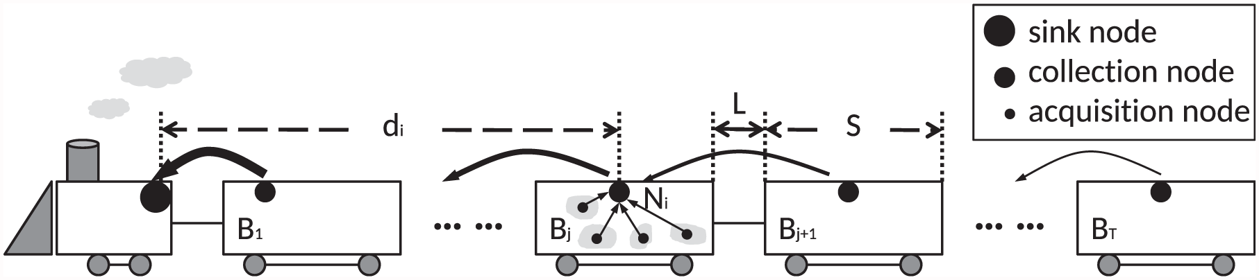
In this article, focusing on a real-life application of WSNs in trains to monitor the goods conditions in a long-distance transportation, we address the linear sensor deployment problem with the goal of maximizing the network lifetime. The linear sensor deployment problem has been studied in several recent works,^18–26 and their solutions can be applied to many real-life applications, such as monitoring railway bridge, highway traffic, and oil pipeline. We study a many-to-one sensor network as shown in Figure 1. In a boxcar, acquisition nodes directly send data to collection nodes which transmit the collected data to the sink node through multi-hop forwarding scheme (since the energy consumed by receiving data from acquisition nodes in each round of data collection can be seen as a constant, we can only manage the energy for sending or relaying data among sink and collection nodes). The lifetime of the WSN can be limited by collection nodes with heavy traffic load or power consumptions. Due to some realistic constraints, the WSNs for monitoring trains differ from most of the existing work in one to several aspects as follows:

Setting collection nodes in boxcars sharply weakens the transmit signal and shortens the transmission range, compared to that in an open field.

To collect data in all boxcars, each boxcar must hold at least one collection node.

All nodes must locate inside boxcars, that is, nodes cannot be placed between any adjacent two boxcars.

Figure 1.

Monitoring a train with sensors.

Hence, the deployment problem of collection nodes in trains becomes even more challenging. We first formulate the problem with realistic discrete power model of nodes as a mixed integer linear programming (MILP) problem. Then, an efficient heuristic to find the transmission level for each collection node is proposed to satisfy the above constraints step by step. The evaluation results show that the heuristic derives nearly the same lifetime as MILP. Moreover, the WSN with appropriate number of nodes can improve its lifetime up to 10.6% for a train with 80 boxcars.

The rest of the article is organized as follows. Section “Problem setting” presents the system model and our assumptions. Section “Sensor deployment for lifetime maximization” discusses the MILP formulation and the efficient heuristic schemes. Section “Evaluation” provides the evaluation results. Section “Real implementation” describes the tested experiment and real implementation of the whole monitoring system. Section “Related work” investigates related work. Section “Conclusion” concludes the article and points out our future work.

Problem setting

A WSN in trains for monitoring long-distance goods transportation consists of three components: acquisition nodes, collection nodes (node for short, if not confused), and sink node, as shown in Figure 1. Collection nodes directly collect and package the data from acquisition nodes in goods. One sink node is fitted in the engine to collect the data forwarded by each collection node, display these data on site, and send them to the remote control center which is mainly responsible for data analysis. The detailed description of the whole monitoring system is shown in section “Real implementation”. Now, we focus on the collection node deployment and provide the corresponding system models.

System model

We consider a WSN consisting of n collection nodes {N₁,…,N_n}, which is used to monitor a train with T boxcars. The length of each boxcar is S, and the distance between two boxcars is L. The closest node to the engine is N₁ and N_n is the furthest one. We further assume that nodes forward the sensing data one by one to the sink node as shown in Figure 1, that is, node N_n sends its data to node N_n − 1, and N_n − 1 sends its own data as well as the relayed data to node N_n − 1, and so on without interweaving transmission among nodes.

Note that, in WSNs, the transmission range of a node directly depends on its transmission power/current. Lots of theoretical studies, such as Olariu and Stojmenovic,⁷ Xing et al.,¹⁴ and Liu and Mohapatra,²¹ have adopted ideal power model which assumed that nodes’ transmission power and range can adjust continuously, where the required transmission power can be modeled as²⁷

P (d) = γ + α d^{β}

where d is the distance between two sensor nodes, γ and α are system-dependent parameters, and 2 ≤ β ≤ 4. In general, γ is a small constant. However, most modern nodes can only adjust their transmission power/current and range discretely, and normally have only a few transmission levels. Nodes implemented in our monitoring system belong to this case. We assume that each node has M transmission levels, which are represented as a vector $ℝ = {(R_{1}, I_{1}^{sd}), ., (R_{M}, I_{M}^{sd})}$ , where R_m is the transmission range when nodes operate at sending current $I_{m}^{sd}$ . While the sending current can regulate discretely, the receiving current is constant and denoted as I^rev. Here, $(R_{M}, I_{M}^{sd})$ is the maximum transmission level while $(R_{1}, I_{1}^{sd})$ is the minimum one. For our case, I^rev is on the same order of $I_{m}^{sd}$ , which is not negligible.

For each round of data collection, the amount of data in each collection node is the same after data packaging, which needs time t to transmit (send or receive). For node N_i, it will take time (n − i) · t to receive the data from all its predecessors, and then take time (n − i+1) · t to send all date to the next node N_i₋₁. Suppose that node N_i operates at transmission level m, the required energy consumption is $E_{i} = t \cdot ((n - i + 1) \cdot I_{m}^{sd} + (n - i) \cdot I^{rev})$ to transmit all the data. Define the energy hole as the node consumes the most energy during each round of data collection. The lifetime of a WSN is determined by the energy hole, which is first depletes its battery among all nodes in the WSN.

As shown in Figure 1, d_i denotes the distance between node N_i and the sink node. d(i,j) = d_j − d_i denotes the distance between nodes i and j. We say a WSN is connected if the transmission range of each node N_i is greater than or equal to the distance between itself and the next node N_i₋₁, that is, d(i − 1, i).

Problem statement

A feasible node deployment of a WSN for monitoring trains has to meet all the three requirements as follows:

A1: there is no null boxcar which holds no node, that is, each boxcar has at least one node.

A2: no node locates outside boxcars.

A3: the deployment should be connected.

To obtain the maximum lifetime of the WSN, we need to find out the optimal number of nodes n, the distances between each two adjacent nodes d(i − 1, i), and the corresponding transmission level, such that the energy consumption of the energy hole is minimized. Note that the distance d(i − 1, i) should be less than or equal to the corresponding transmission range of N_i. The feasible deployment with maximum lifetime is called optimal deployment. Due to the NP-hardness of the problem, we first formulate this problem as a MILP problem, then develop efficient heuristics.

Sensor deployment for lifetime maximization

Since the data density in nodes varies, that is, more data need to relay/transmit for nodes closer to the sink node and vice verse, unevenly distributing nodes and balancing the energy consumption at each node can further prolong the lifetime of a WSN compared to equal-distance distributing. Following this idea, some research works, such as Liu and Mohapatra²¹ and Guo et al.,²² have addressed the linear sensor deployment problem, where nodes can be placed anywhere along a continuous pipeline. However, nodes can locate segmentally in boxcars for train monitoring to meet the requirements above. Hence, not all the transmission levels in ℝ is necessary, and Lemma 1 presents the lower and upper bound of transmission range for any feasible sensor deployment.

Lemma 1. The lower bound R^low (upper bound R^up) of the transmission ranges of all nodes in a feasible deployment is the closest range value larger than L (2S+L) in vector ℝ.

Proof. In a feasible deployment, since the distance of two adjacent nodes in different boxcars is larger than or equal to L, the adjacent nodes with distance of less than L must locate in the same boxcar. Then, the transmission range of the first node N₁ must be larger than or equal to L due to its location in boxcar S₁. Moreover, if some nodes from N₂ to N_n have transmission range less than L, their transmission range can be increased to L without affecting the WSN’s lifetime due to their energy consumption lower than that of node N₁. Therefore, the R^low holds.

For upper bound, if the distance of two adjacent nodes is larger than 2S+L, between the two nodes, there must be at least one boxcar with no node inside, which contradicts the connected deployment. Therefore, the R^up also holds.

After bounding the transmission level by Lemma 1, denote the transmission vector as $ℝ = {(R_{1}, I_{1}^{sd}), ., (R_{K}, I_{K}^{sd})}$ , where R₁ = R^low and R_K = R^up. As shown in Guo et al.,²² the optimal number deriving maximum lifetime of a WSN monitoring pipeline falls in an interval. This may also be true for WSNs in train monitoring, and Lemma 2 shows the possible interval for this case.

Lemma 2. The optimal number of nodes must be in the interval of $[T, ⌈ \frac{T \cdot (I_{K}^{sd} + I^{rev})}{I_{1}^{sd} + I^{rev}} ⌉]$ .

Proof. To guarantee requirement A1, there must be at least T nodes. As the number n of nodes increases, the data relayed grow. Hence, when the energy consumption of node N_i operating at level 1 becomes greater than that of node N_i operating at level K, increasing the number n will definitely increase energy consumption and shorten the WSN’s lifetime. That is

\begin{matrix} \forall i, (n - i) \cdot I_{1}^{sd} + (n - i + 1) \cdot I^{rev} \\ > (T - i) \cdot I_{K}^{sd} + (T - i + 1) \cdot I^{rev} \\ \Rightarrow n > max {\frac{T \cdot (I_{K}^{sd} + I^{rev}) - (i - 1) \cdot (I_{K}^{sd} - I_{1}^{sd})}{I_{1}^{sd} + I^{rev}} | \forall i} \\ \Rightarrow n > \frac{T \cdot (I_{K}^{sd} + I^{rev})}{I_{1}^{sd} + I^{rev}} \end{matrix}

Therefore, the lemma holds.

For each value n in the interval derived by Lemma 2, we first formulate an MILP problem, and then propose an efficient heuristic.

MILP formulations

For each node N_i, define several binary variables:

x_ij = 1 if node N_i locates at boxcar B_j, or x_ij = 0.

y_ik = 1 if node N_i operates at transmission level k, or y_ik = 0.

Each node can locate in only one boxcar

\begin{matrix} \forall i \in [1, n], \sum_{j = 1}^{T} x_{ij} = 1 \end{matrix}

(1)

Each node can operate at only one transmission level

\begin{matrix} \forall i \in [1, n], \sum_{k = 1}^{K} y_{ik} = 1 \end{matrix}

(2)

As requirement A1, in order to obtain the data for all boxcars, there is at least one node in each boxcar

\begin{matrix} \forall j \in [1, T], \sum_{i = 1}^{n} x_{ij} \geq 1 \end{matrix}

(3)

As requirement A2, the distance between the sink node and the node in boxcar B_j must be in the range between left and right walls of B_j

\begin{matrix} \forall i \in [1, n], d_{i} \geq \sum_{j = 1}^{T} x_{ij} \cdot (j \cdot L + (j - 1) \cdot S) \\ \forall i \in [1, n], d_{i} \leq \sum_{j = 1}^{T} x_{ij} \cdot j \cdot (L + S) \end{matrix}

(4)

As requirement A3, the transmission range of node N_i₊₁ must be greater than or equal to the distance between itself and node N_i

\begin{matrix} \forall i \in [1, n - 1], \sum_{k = 1}^{K} y_{(i + 1) k} \cdot R_{k} \geq d_{i + 1} - d_{i} > 0 \end{matrix}

(5)

The energy consumption of each node N_i is expressed as

\begin{matrix} E_{i} = (n - i + 1) \cdot \sum_{k = 1}^{K} y_{ik} \cdot I_{k}^{sd} + (n - i) \cdot I^{rev} \end{matrix}

(6)

We denote the energy hole as E^max =max{E_i|i = 1,…,n}. That is, our objective is to minimize the energy of energy hole

\begin{matrix} \min E^{\max} \end{matrix}

(7)

Conditions (1)–(6) form a constraint set, and combined with the optimization objective in condition (7), it forms an MILP problem.

An efficient heuristic

Since the distance d(i − 1, i) between any two adjacent nodes, that is, the transmission range of node N_i, cannot exceed 2S+L, we reassign the transmission range R_K as 2S+L but unchange $I_{K}^{sd}$ following Lemma 1. Moreover, after the reassignment, we have

Lemma 3. There is no two continuous boxcars holding no node for any connected deployment.

Now, we will present a two-step heuristic to meet those requirements step by step.

Step 1. This step is to deploy nodes to cover the whole train range and to guarantee requirements A1 and A3. We propose a recursive algorithm to deal with this step. Each sub-problem cover(nd, cov, tn) consists of six sub-steps, which uses nd nodes to cover a train with tn boxcars and range of cov. The three variables are updated in every recursion.

Step 1.1: Here, we assume the cover range of a train as a continuous one-dimensional space and do not differentiate the space inside or between boxcars, that is, the node can be placed anywhere along the train. By this assumption, we use the algorithm L2H or H2L (Algorithm 1 or 2 in Guo et al.²²) to deploy nodes to cover the range of cov.

Algorithm 1 Expansion: L2H heuristic algorithm.
Input: nd, cov and ℝ;
Output: transmission level assignment vector V;
1: ifnd · R_K < covthen
2: exit: the input parameters are infeasible;
3: end if
4: Initialize V = <nd,0,…,0 >;
5: while $\sum_{i = 1}^{K} (c_{i} \cdot R_{i}) < L$ do
6: $E^{\min} = nd \cdot t \cdot I_{K}^{sd}$ ;
7: fori = 1 toK − 1 do
8: $E_{tmp} = I_{i}^{sd} \cdot t \cdot (1 + \sum_{j = i + 1}^{K} c_{j})$ ;
9: ifc_i ≠ 0 and E_tmp ≤ E^minthen
10: E^min = E_tmp; x = i;
11: end if
12: end for
13: Update assignment vector: c_x− = 1; c_x + 1+ = 1;
14: end while

Algorithm 2 Contraction: H2L heuristic algorithm.
Input: nd, cov and ℝ;
Output: transmission level assignment vector V;
1: ifnd · R_K < covthen
2: exit: the input parameters are infeasible;
3: end if
4: Initialize V = <0,…,0, nd>;
5: while $\sum_{i = 1}^{K} (c_{i} \cdot R_{i}) > L$ do
6: $E^{\max} = nd \cdot t \cdot I_{1}^{sd}$ ;
7: fori = 1 toKdo
8: $E_{tmp} = I_{i}^{sd} \cdot t \cdot (\sum_{j = i}^{K} c_{j})$ ;
9: ifc_i ≠ 0 and E_tmp≥E^maxthen
10: E^max = E_tmp; x = i;
11: end if
12: end for
13: ifx == 1 or $\sum_{i = 1}^{K} (c_{i} \cdot R_{i}) < cov + (R_{x} - R_{x - 1})$ then
14: break;{no more contraction is needed;}
15: else
16: Update assignment vector: c_x− = 1; c_x₋₁+ = 1;
17: end if
18: end while

To be self-contained, we include the two algorithms (L2H or H2L) and provide brief explanation for them. Algorithms 1 and 2 show the algorithms adapted to the notations used in this article. The vector V = <c₁,…,c_K > denotes the number of sensors assigned in each transmission level. There is $\sum_{i = 1}^{K} = nd$ .

Algorithm L2H

This algorithm expands nodes’ transmission levels from low to high. First, if the nodes are not enough to cover the desired range cov, the algorithm exits because of no feasible solution (lines 1–3). Otherwise, the algorithm initializes the transmission level assignment vector V such that all nodes transmit at the lowest level (line 4). If the current level assignment cannot cover the desired range cov, appropriate nodes will be selected to increase their transmission levels (lines 6–13). When the while loop exits, the vector V will contain the transmission level assignment.

Algorithm H2L

This algorithm contracts nodes’ transmission levels from high to low. Instead, the initial assignment vector is V = <0,…,0, nd > (line 4). While the coverage of nodes is larger than the range cov, we decrease the transmission level of the energy hole node that consumes the most energy until no further improvement to the lifetime can be obtained. The steps of this algorithm are similar to those in Algorithm L2H except that it tries to find the energy hole node (lines 6–11) and reduce its transmission level.

After step 1.1, there are some key properties of the current deployment shown as follows:

Lemma 4. The transmission range of node N_i₊₁ is greater than or equal to that of N_i, that is, d(i − 1, i) ≤ d(i, i+1).

Proof. This Lemma can be derived directly according to Theorem 1 in Guo et al.²²

Theorem 5. There are no boxcar that holds more than one node from the first null boxcar to the last boxcar B_tn in the currently considered train range.

Proof. The distance between the two nodes adjacent to a null boxcar must be larger than S, while the distance is smaller than S if two nodes locate inside a single boxcar. If two nodes locate in the same boxcar between the first null boxcar to the last boxcar B_tn, it contradicts Lemma 4. Therefore, the theorem holds.

In sum, the deployment by this sub-step only meets requirement A3. There may be some boxcar holds no node, as shown in Figure 2(a). We will modify the deployment to meet the requirement A1 in the following sub-steps.

Figure 2.

Step 1: to guarantee requirement A1: (a) Step 1.1: the deployment only meets A3, (b) Step 1.2: all nodes are moved leftward, and (c) Step 1.4: moving nodes until all boxcars hold nodes.

Step 1.2: Since we consider discrete transmission model, the cover range of the current deployment may be larger than cov. Hence, we move all nd nodes leftward until the last node N_nd just covers the train range of cov. Suppose that N_nd moves δ meters leftward. Then, update the corresponding distance d_i of each node to the sink node by

d_{i} = (d_{i} - δ < L) ? L : d_{i} - δ

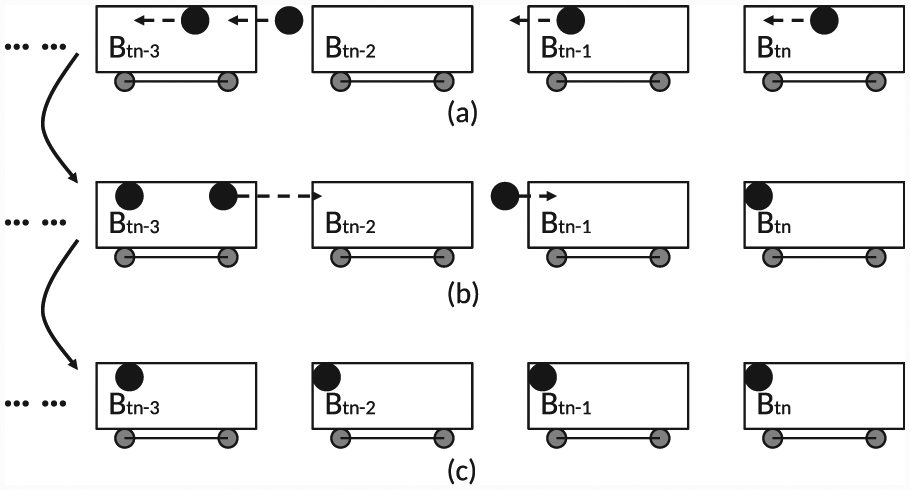
Hence, the distance between any two adjacent nodes becomes smaller or keeps unchanged, and the energy consumption of energy hole also decreases or remains unchanged. All nodes in Figure 2(a) are moved leftward, and the deployment becomes the one in Figure 2(b).

Step 1.3: Find the first null boxcar from B₁ to B_tn, and denote its index as I_null. For example, I_null equals tn − 2 in Figure 2(b). If find no one, return.

Step 1.4: Check boxcars from B_tn₋₁ to B₁ and move nodes rightward or leftward until all boxcars from B_Inull to B_tn hold nodes. Let the current null boxcar be B_j. If one node locates between B_j and B_j₊₁, move the node to the right wall of B_j. Or, move the node just before B_j rightward to the left wall of B_j. Then, update d_i of nodes in B_(Inull+1) to B_tn accordingly. The deployment becomes to Figure 2(c) by moving two nodes rightward of Figure 2(b). Since the null boxcar can only appear within the interval from the first null boxcar to last one according to Theorem 5, checking boxcars from tail to head boxcar, needs less node movements. More precisely, at most one node needs to move in each iteration (of checking each boxcar). Hence, there are at most tn nodes need to move if checking from tail to head boxcar. By contrast, if in an opposite direction, more nodes have to move in an iteration when encountering a null boxcar. For example, moving one node to a null boxcar will make the original former null boxcars, which hold nodes now, null again, thus other nodes have to move to fill them again. Hence, it needs more movements. We use n_left to denote the number of nodes in the left of the boxcar B_Inull after this sub-step.

Step 1.5: Update the three variables nd, cov, tn as follows:

nd⇐n_left;

tn⇐I_null;

For the current deployment, if the node in boxcar B_Inull locates at the left wall, cov⇐I_null⇐L+(I_null − 1) · S; if the node locates at the right wall, cov⇐I_null · (L+S);

Step 1.6: Conduct recursion: cover(nd, cov, tn).

After Step 1.4, the location or distance to the sink node of the collection nodes in boxcars from B_Inull to B_tn should be fixed, because moving them in the next recursion may not lead to better solutions, which is also indicated by the evaluation results. Hence, we choose the current first null boxcar as the last boxcar of the next recursion. In addition, the recursion can definitely terminate, since at the worst case, it would terminate at the sub-problem where there was one node left to cover one boxcar.

Note that for each sub-problem, we keep the data density of each node unchanged as the initial, that is, N_i always receive n − i and send n − i+1 data. The complete algorithm of Step 1 to cover T boxcars by n nodes is shown in Algorithm 3. First, the algorithm makes initialization with parameters that cover the whole train with T boxcars using n sensor nodes (line 1). It then conducts recursion by calling function cover(nd, cov, tn) recursively in line 2. Line 3 conducts an update by setting the energy hole as the sensor node that consumes the most energy. To meet the requirement A3 (i.e. a connected network), line 4 updates each node’s transmission level to R_j that satisfies R_j₋₁ < d(i − 1, i) ≤ R_j. That is, line 4 adjusts each node’s level to the one with a transmission range just larger than or equal to the distance between itself and next node.

Algorithm 3 Step 1.
1: Initialization: d_i⇐ 0, nd⇐n, tn⇐T, cov⇐ (T − 1) · S + T · L;
2: cover(nd, cov, tn);
3: Update the energy hole;
4: Update transmission levels to meet requirement A3;

Step 2. This step is to guarantee requirement A2 for the deployment derived by Step 1.

First, from N₁ to N_n, move nodes in-between two adjacent boxcars (B_j and B_j₊₁) leftward or rightward to make them be inside boxcars, as shown in Figure 3. Move one node rightward to the left wall of boxcar B_j₊₁, if it will not become a new energy hole. Or, move it leftward to the right wall of boxcar B_j. Then, update the energy hole and transmission level of each node accordingly.

Figure 3.

Step 2: to guarantee requirement A2.

The time complexity of the two-step heuristic scheme is O(n²K²), of which the detailed analysis is shown as follows. For Step 1, the time complexity of sub-steps from 1 to 5 is as follows: O(nd · K²), O(nd), O(tn), O(tn), and O(1), respectively. Due to nd ≥ tn, the time complexity of each sub-problem is dominated by Step 1.1 and equals O(nd · K²). Moreover, the time complexity of Step 2 is O(n). Therefore, the time complexity of the overall algorithm is dominated by Step 1, that is, the recursive algorithm cover(), of which the time complexity is analyzed as follows.

In the worst case, the first null boxcar always appears right before the last boxcar B_t in each sub-problem. Hence, the time complexity of each step of recursion is as follows: O(nK²), O((n − 1)K²),…. In all, the total complexity can be calculated as

\begin{matrix} O (n K^{2} + (n - 1) K^{2} + \dots + K^{2}) \\ \Rightarrow O (\frac{n (n + 1)}{2} K^{2}) \\ \Rightarrow O (n^{2} K^{2}) \end{matrix}

Discussions

In practice, sensor nodes may be only installed at some certain locations. For example, put nodes around the air vents of boxcars to enhance transmission signal. In addition, to obtain accurate data, the number of nodes in each boxcar may require to be greater than a threshold value. To deal with these additional requirements or constraints, we can partition a boxcar into a certain number of virtual segments, each of which can be seen as a new boxcar. As shown in Figure 4, a boxcar is partitioned into four segments. Hence, our approaches (both the MILP and the two-step heuristic scheme) proposed can be easily adapted to these realistic cases through the boxcar partition.

Figure 4.

A segmented boxcar.

Evaluation

In this article, we consider eight transmission levels as shown in Table 1. Here, the corresponding current values are obtained from the data sheet of TI RF Transceiver CC1101.²⁸ The transmission range R_k are measured values when the collection nodes around air vents in boxcars are set, which is sharply shorter than that in an open field due to the weakened transmission signal. For a train, the number of boxcars can range from several to 100. The length of one boxcar usually ranges from 9.9 to 17.6 m, and the distance between two boxcars is around 0.6 m.

Table 1.

Sending and receiving current and transmission ranges when transceiver runs at 433 MHz.

Level	1	2	3	4	5	6	7	8
R(m)	1.7	3.0	7.3	10.0	12.7	15.0	19.3	23.3
I^sd(mA)	11.9	12.4	13.1	14.4	15.9	19.4	24.2	29.1
I^rev(mA)	15.7

The ILOG CPLEX solver has been exploited to obtain the optimal solution from the MILP formulation, compared to which, we evaluate the performance of the proposed two-step heuristic scheme on prolonging the WSN’s lifetime. Figure 5 shows the normalized lifetime of the WSN for different number of nodes in the interval given by Lemma 2. The optimal lifetime derived by MILP for the WSN with T nodes is used as the baseline.

Figure 5.

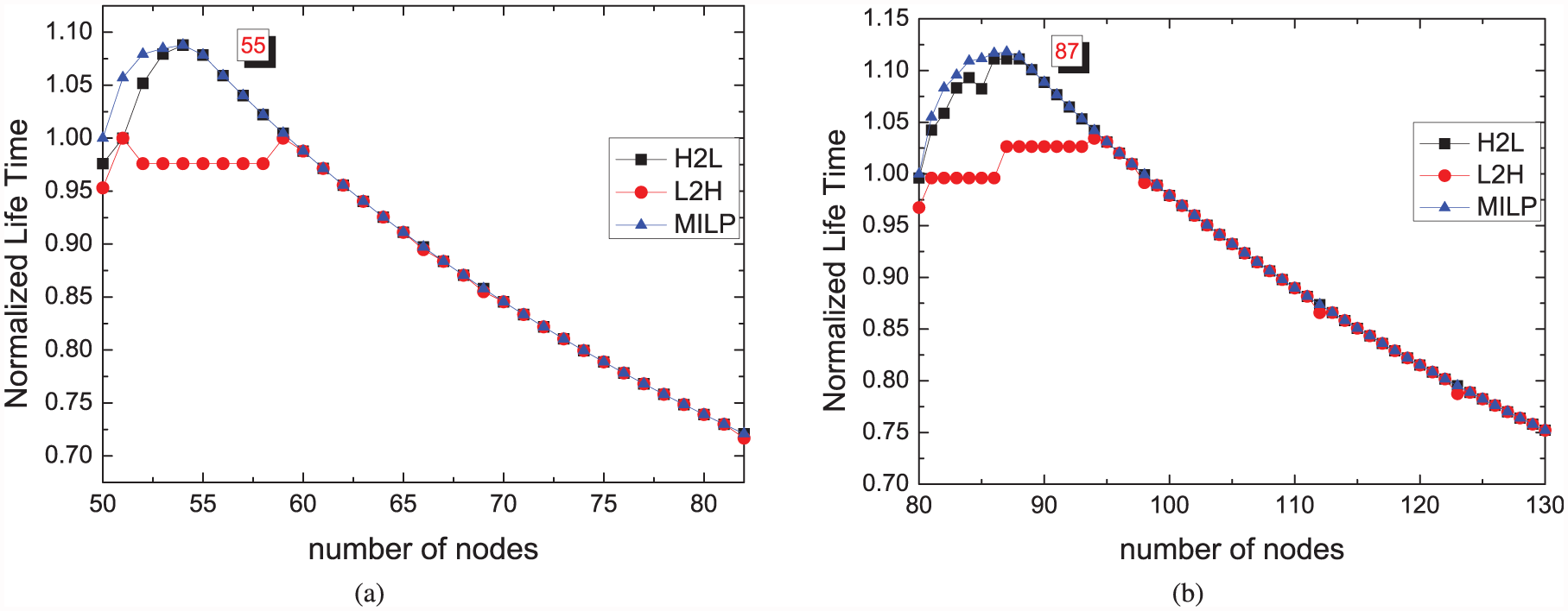
Normalized lifetime for two-step heuristic schemes and MILP. The optimal number of nodes is shown in shadowed text box: (a) T = 50, S = 15 and (b) T = 80, S = 15.

From the results, we can see that the WSN’s lifetime improves as the number of nodes increases. When it reaches an appropriate number of nodes, the WSNs lifetime can be improved by up to 10.6% compared to that for the minimum number when T = 80. However, if more than the appropriate number of nodes are deployed, the WSN’s lifetime reduces as the number of nodes increases due to more energy being consumed in the energy hole to transmit the additional data. Therefore, there is an optimal number of nodes to achieve the maximum lifetime of the WSN, such as 55 nodes for T = 50 and 87 nodes for T = 80, more nodes may not always help improve WSNs’ lifetime.

In addition, our two-step heuristic scheme combined with H2L, labeled as H2L in Figure 5, performs almost the same as the optimal MILP solution, while the one combined with L2H, labeled as L2H in the figure, performs slightly worse. To analyze the results, there are two questions here that we have to answer:

Why the heuristic combined with H2L is better than the one with L2H?

Why they still have very good performance even when considering those realistic constraints, such as requirements A1 and A2?

For the first question, the heuristic H2L aims at minimizing the energy consumption for the node that consumes the most energy in each iteration, which complies with the goal of the initial problem. While L2H follows a different direction by choosing the node that consumes the minimum energy and increasing its power level in each interaction, which leads to irreversible energy consumption jump. The similar reasons have also been presented for the result analysis in the previous work of Guo et al.²²

For the second question, there are three main reasons. First, we combine the two good heuristic schemes (H2L and L2H) into each step of recursion. Second is on our choice of when and where to conduct recursion. Since there are usually no enough nodes to cover those boxcars in the interval from the first null boxcar to the last boxcar when n is relatively small, the location of one node is fixed at the left or right wall of one boxcar in this interval, that is, its transmission level is also fixed after Step 1.4. Hence, we can only manage the transmission levels of nodes before the first null boxcar, and choose it as the last boxcar of the next sub-problem. In addition, when n is relatively large, it will conduct few recursions. Third, in Step 2, we move one node in-between two adjacent boxcars to avoid to generate a new energy hole as far as possible.

Real implementation

The Monitoring System for Long-Distance Goods Transportation consists of three layers: sensing layer, communication layer, and application layer, as shown in Figure 6. The collected data in the sensing layer are transmitted to the application layer through GPRS and Internet in the communication layer. The control center in application layer is implemented to store, analyze, and display data obtained from all trains monitored. In what follows, we will detail the local monitoring system for a train in sensing layer.

Figure 6.

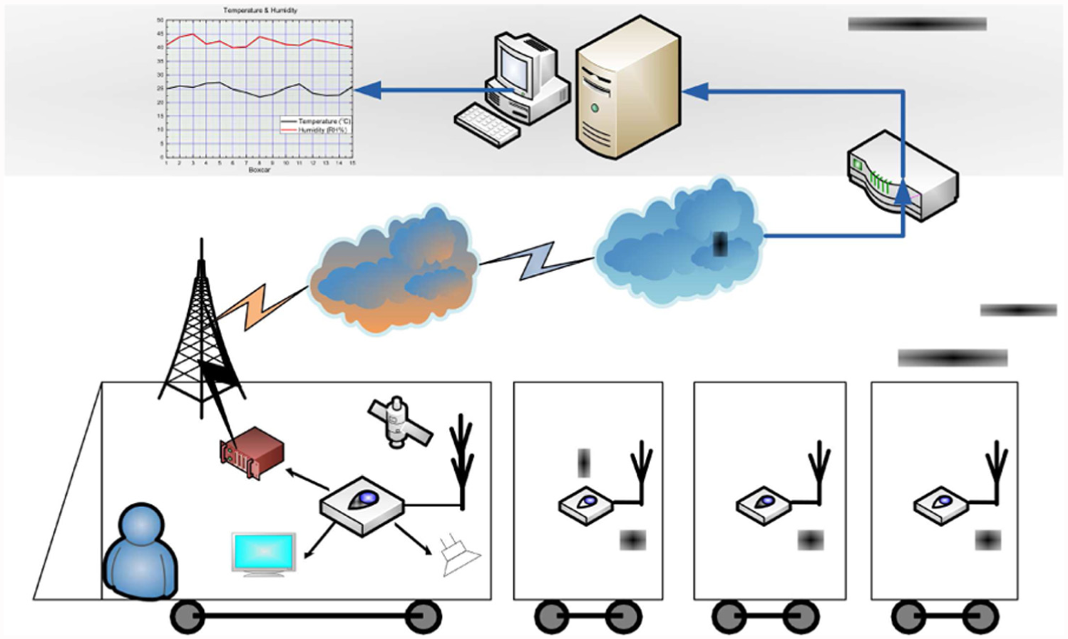
Monitoring system for long-distance goods transportation. Acquisition nodes are not shown.

We have designed and implemented two types of node: TYP1 and TYP2, as shown in Figure 7(a). TYP1 adopts a low-power MCU MSP430, CC1101 transceiver chip, and temperature and humidity sensor SHT15 and is powered by a high-temperature lithium battery. Besides an MCU MSP430 and transceiver CC1101, TYP2 also integrates a 64*128 dot matrix ST7565 LCD, GPS module Gstar-GS-89m-J, and GPRS module MC52i. TYP1 node limits the lifetime of the WSN in sensing layer. Collection and acquisition nodes in boxcars adopt TYP1, while the sink node employs TYP2. Currently, a set of collection nodes have been installed around air vents in boxcars following the solution derived by the proposed heuristic scheme. The acquisition nodes will be put into goods, such as cotton package, when to load them onto the boxcars.

Figure 7.

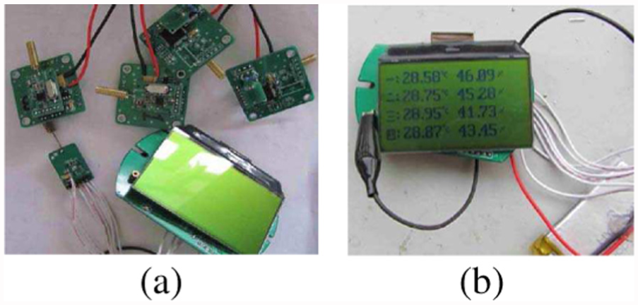
A tested experiment using one sink node and four collection nodes: (a) TYP1 and TYP2 nodes and (b) temperature and humidity data.

The temperature and humidity data are collected every 5 min and nodes switch to sleep mode for energy conservation after each round of data collection. Collection nodes forward these data to the sink node which provides several functions as follows:

Display the obtained data on site. On LCD, the first column is indices for boxcars, the second is for temperature data, and the last is for humidity data, as shown in Figure 7(b).

Examine the obtained data. If the temperature and/or humidity of one boxcar is higher or lower than a threshold, it sounds alarm and the worker may heat or cool the boxcar.

Insert the location information (longitude and latitude) into the data packet, which is then sent to the remote control center through GPRS module.

We have performed tested experiments for one sink node and four collection nodes, as shown in Figure 7(a). We numbered the four nodes and put them linearly at four different sites around our laboratory. Figure 7(b) shows the temperature and humidity of the four monitored sites, where the top row on LCD corresponds to data of the first node that is closest to the sink node, and the second row is for the second node, and so on. For an accelerated test, each node is set to transmit data continuously at maximum transmission level, where the lifetime of the WSN is around 1 day, for a battery with capacity of 1.2 Ah. This indicates that one WSN equipped with only collection nodes and consisting of 100 boxcars can operate for at least 1000 days under normal situation for the battery of same capacity when the data are collected in a period of 5 min.

Related work

In this section, we investigate existing works that study linear sensor deployment problem, which is the research thread most related to this work. Ganesan et al.¹⁸ consider the problem of jointly optimizing sensor placement and transmission structure for data collection. The authors propose an analytical solution for sensor networks with linear topology. Perillo et al.²⁰ investigate the transmission range distribution optimization problem with a goal to maximize the lifetime of many-to-one WSNs. The authors propose a solution that determines what fraction of packets each node should send over different distances. Liu and Mohapatra²¹ discuss how to deploy back-haul nodes for wireless networks with energy constraints. Specially, the studied problem is to achieve the minimum number of nodes needed to cover a back-haul network given the requirements of lifetime, energy, and covered area. The authors propose a greedy approach that has near-optimal performance. Jawhar et al.²³ consider the delay-tolerant linear sensor networks with mobile nodes and study different movement approaches for these nodes to optimize the delay of data collection. Alduraibi et al. ²⁶ investigate the optimization models for determining the sensor node density with three different objectives: achieving desired detection fidelity with the minimum number of nodes, determining nodes’ placement to maximize the coverage, and minimizing the number of nodes for non-uniform fidelity. The authors propose a general formulation framework that can solve all the three optimization models.

All works, including Ok et al.,¹⁹ Guo et al.,²² Wu et al.,²⁴ and Xia et al.,²⁵ study WSNs for pipeline monitoring but they have different focuses. Ok et al.¹⁹ consider self-sustainable sensors and try to minimize the number of sink nodes in the sensor network. Xia et al.²⁵ also consider self-sustainable sensors but try to minimize the cost of energy harvesting device. Guo et al.²² focus on battery-powered sensors and try to maximize the lifetime of the senor network. Wu et al.²⁴ discuss channel-aware relay node placement and try to minimize the power consumption of sensing nodes. All the above works study WSNs with linear topology, but confine to one continuous dimension, that is, nodes can be placed anywhere along the linear space. However, different with them, our work studies a disconnected dimension, where nodes can only be placed inside boxcars and not outside boxcars (i.e. the space between two boxcars). Because of this difference, existing approaches cannot be directly applied to our problem.

Conclusion

In this article, we have discussed the linear sensor deployment problem to maximize the lifetime of WSNs in trains for monitoring long-distance goods transportation. Taking account of several realistic requirements, we presented the lower and upper bounds for both the transmission range and the number of nodes, between which the optimal solution must fall. Based on this, we first formulated the problem as a MILP problem, and then proposed a two-step efficient heuristic scheme which met the requirements step-by-step. The evaluation results show that the proposed heuristic combined with H2L performed nearly the same as the optimal MILP solution, while the one with L2H performed slightly worse. In addition, the WSN with appropriate number of nodes can prolong its lifetime by up to 10.6% for a train with 80 boxcars. We also discussed a tested experiment in a laboratory environment, as well as the real implementation of the whole monitoring system. For our future work, we plan to study the multi-hop scheme with interleaved data forwarding and adapt our monitoring system to more real-life applications.

Footnotes

Academic Editor: Amiya Nayak

Declaration of conflicting interests

The author(s) declared no potential conflicts of interest with respect to the research, authorship, and/or publication of this article.

Funding

The author(s) disclosed receipt of the following financial support for the research, authorship, and/or publication of this article: This work was supported in part by the National Natural Science Foundation of China under grant numbers 61472072, 61528202, and 61502474.

References

Mainwaring

Culler

Polastre

. Wireless sensor networks for habitat monitoring. In: Proceedings of the ACM international workshop on wireless sensor networks and applications, Atlanta, GA, 28 September 2002, pp.88–97. New York: ACM.

Tolle

Polastre

Szewczyk

. A macroscope in the redwoods. In: Proceedings of the international conference on embedded networked sensor systems, San Diego, CA, 2–4 November 2005, pp.51–63. New York: ACM.

Chebrolu

Raman

Mishra

. Brimon: a sensor network system for railway bridge monitoring. In: Proceedings of the international conference on mobile systems, applications, and services, Breckenridge, CO, 17–20 June 2008, pp.2–14. New York: ACM.

Kong

Liu

. A survey on green-energy-aware power management for datacenters. ACM Comput Surv 2014; 47(2): 1–38.

Jin

Xia

. Mixed criticality scheduling for industrial wireless sensor networks. Sensors 2016; 16(9): 1–20.

Akyildiz

Sankarasubramaniam

. A survey on sensor networks. IEEE Commun Mag 2002; 40(8): 102–114.

Olariu

Stojmenovic

. Design guidelines for maximizing lifetime and avoiding energy holes in sensor networks with uniform distribution and uniform reporting. In: Proceedings the IEEE international conference on computer communications, Anchorage, AK, 6–12 May 2007, pp.1–12. New York: IEEE.

Vicaire

Cao

. Achieving long-term surveillance in vigilnet. ACM Trans Sens Netw 2009; 5(1): 1–39.

Basagni

Carosi

Melachrinoudis

. Controlled sink mobility for prolonging wireless sensor networks lifetime. Wirel Netw 2008; 14(6): 831–858.

10.

Gandham

Dawande

Prakash

. Energy efficient schemes for wireless sensor networks with multiple mobile base stations. In: Proceedings of the IEEE global telecommunications conference (vol. 1), San Francisco, CA, 1–5 December 2003, pp.377–381. New York: IEEE.

11.

Bozdag

Ekici

. Partitioning based mobile element scheduling in wireless sensor networks. In: Proceedings of the annual IEEE Communications Society conference on sensor and ad hoc communications and networks, Santa Clara, CA, 26–29 September 2005. pp.386–395. New York: IEEE.

12.

Yang

. SenCar: an energy-efficient data gathering mechanism for large-scale multihop sensor networks. IEEE T Parall Distr 2007; 18(10): 1476–1488.

13.

Wang

Srinivasan

Chua

. Using mobile relays to prolong the lifetime of wireless sensor networks. In: Proceedings of the annual international conference on mobile computing and networking, Cologne, 28 August–2 September 2005, pp.270–283. New York: ACM.

14.

Xing

Wang

Xie

. Rendezvous planning in mobility-assisted wireless sensor networks. In: Proceedings of the IEEE international real-time systems symposium, Tucson, AZ, 3–6 December 2007, pp.311–320. New York: IEEE.

15.

Zhao

Ammar

. Message ferrying: proactive routing in highly-partitioned wireless ad hoc networks. In: Proceedings of the IEEE workshop on future trends of distributed computing systems, San Juan, Puerto Rico, USA, 28–30 May 2003, pp.308–314. New York: IEEE.

16.

Jin

Zhang

Zeng

. Collision–free multichannel superframe scheduling for IEEE 802.15. 4 cluster–tree networks. Int J Sens Netw 2014; 15(4): 246–258.

17.

Zhu

Guo

Tosun

. Multi-path planning for mobile element to prolong the lifetime of wireless sensor networks. In: Proceedings of the IEEE international conference on embedded and real-time computing systems and applications, Beijing, China, 24–26 August 2009, pp.41–50.

18.

Ganesan

Cristescu

Beferull-Lozano

. Power-efficient sensor placement and transmission structure for data gathering under distortion constraints. In: Proceedings of the international symposium on information processing in sensor networks, Berkeley, CA, 26–27 April 2004, pp.142–150. New York: ACM.

19.

Thadakamalla

Raghavan

. Optimal transmission power in self-sustainable sensor networks for pipeline monitoring. In: Proceedings of the IEEE international conference on automation science and engineering, Scottsdale, AZ, 22–25 September 2007, pp.591–596. New York: IEEE.

20.

Perillo

Cheng

Heinzelman

. On the problem of unbalanced load distribution in wireless sensor networks. In: Proceedings of the IEEE global telecommunications conference workshops, Dallas, TX, 29 November–3 December 2004, pp.74–79. New York: IEEE.

21.

Liu

Mohapatra

. On the deployment of wireless data back-haul networks. IEEE T Wirel Commun 2007; 6(4): 1426–1435.

22.

Guo

Kong

Zhu

. Sensor placement for lifetime maximization in monitoring oil pipelines. In: Proceedings of the ACM/IEEE international conference on cyber-physical systems, Stockholm, 12–15 April 2010, pp.61–68. New York: ACM.

23.

Jawhar

Ammar

Zhang

. Ferry-based linear wireless sensor networks. In: Proceedings of the IEEE global communications conference, Atlanta, GA, 9–13 December 2013, pp.304–309.

24.

Chatzigeorgiou

Youcef-Toumi

. Channel-aware relay node placement in wireless sensor networks for pipeline inspection. IEEE T Wirel Commun 2014; 13(7): 3510–3523.

25.

Xia

Liu

Deng

. Cost minimization of wireless sensor networks with unlimited-lifetime energy for monitoring oil pipelines. IEEE/CAA J Automat Sin 2015; 2(3): 290–295.

26.

Alduraibi

Lasla

Younis

. Coverage-based node placement optimization in wireless sensor network with linear topology. In: Proceedings of the IEEE international conference on communications, Kuala Lumpur, Malaysia, 23–27 May 2016, pp.1–6.

27.

Rappaport

. Wireless communications: principles and practice. Upper Saddle River, NJ: Prentice Hall, 1996.

28.

TI RF Transceiver CC1101. http://focus.ti.com/docs/prod/folders/print/cc1101.html, 2010.