Sage Journals: Discover world-class research

Abstract

Robotic sensor deployment is fundamental for the effectiveness of wireless robot sensor networks-a good deployment algorithm leads to good coverage and connectivity with low energy consumption for the whole network. Virtual force-based algorithms (VFAs) is one of the most popular approaches to this problem. In VFA, sensors are treated as points subject to repulsive and attractive forces exerted among them-sensors can move according to imaginary force generated in algorithms. In this paper, a virtual spring force-based algorithm with proper damping is proposed for the deployment of sensor nodes in a wireless sensor network (WSN). A new metric called Pair Correlation Diversion (PCD) is introduced to evaluate the uniformity of the sensor distribution. Numerical simulations showed that damping can affect the network coverage, energy consumption, convergence time and general topology in the deployment. Moreover, it was found that damping effect (imaginary friction force) has significant influence on algorithm outcomes. In addition, when working under approximate critical-damping condition, the proposed approach has the advantage of a higher coverage rate, better configurational uniformity and less energy consumption.

Keywords

Robot Sensors Wireless Sensor Networks Sensor Deployment Virtual Force Spring Force

1. Introduction

Due to its low power consumption, low cost, and distributed and self-organizational properties, WSNs have became a technology with a wide range of potential applications in both civilian and military areas. WSNs typically consist of a large number of low-cost, low-power sensors with the ability to sense and communicate, and can be used for target tracking, environment monitoring, national defence and underwater detecting, etc. As such, it has been an active research area of interest recently [1,2]. Since robot sensors have the advantage of mobility, intelligence and flexibility, some researchers have considered the use of mobile robots as sensors, especially for hazardous and unmanned environments.

Sensors could be mounted on mobile robots which will then deploy themselves using specific algorithms. Sensor deployment is a key issue for WSNs. The goals of an intelligent sensor deployment algorithm can be summarized according to the following aspects. The first and most important aspect is the conservation of the energy of the sensors. The reduction of energy consumption indicates the extension of the lifetime of network systems. The energy stored in mobile sensors will be utilized for both movement and communication, such that the applied algorithm should be simple to implement and the distance travelled by the sensors should be restricted. The second goal is a uniform network topology, which could help in enlarging the coverage area as well as in reducing the difference in the energy consumption rate for sensing and communication, thus prolonging the lifetime of the whole network. A region with a larger-than-average node intensity will lead to the inefficient use of sensors and impair the detection of other regions. The last goal is shortening the duration of deployment process. Some time-critical applications of WSN detection, such as disaster detection and military usage, require the network to respond quickly to emergency events. Because of all the requirements listed above, the design of a sensor deployment algorithm becomes a challenging task.

With the motility of robot sensors, movement-assisted sensor deployment algorithms can be applied. In this kind of deployment algorithm, each sensor knows its position; the mobile sensors can communicate with each other and can move to other positions according to the information collected in order to improve the coverage ratio. Many approaches have been proposed for movement-assisted sensor deployment [3,4], such as virtual force-based [5 –13], swarm intelligence [14 –18], and computational geometry [19], or else some combination of the above approaches [20,21]. Among these, virtual force-based strategies have emerged as one of the most effective solutions. In this paper, a VFA-based sensor deployment algorithm using spring-like force is proposed and a shielding rule for choosing neighboring sensors is adapted. Mutual force will be generated between each pair of neighboring sensors and will push them to move. Virtual friction force (damping) plays a crucial role in the process of sensor deployment. Through theoretical analysis and computer simulation, we found that with a damping value around critical damping, the proposed algorithm has the best performance. A new metric called ‘pair correlation diversion’ is introduced to evaluate the uniformity of the node distribution. Simulation results showed that the proposed approach exhibited good performance in terms of coverage rate, convergence time and uniformity of configuration.

The rest of this paper is organized as follows: Section 2 introduces the basic concept of the virtual-force algorithm; Section 3 discusses the evaluation metric for the deployment algorithm; the proposed spring force-based algorithm is introduced in Section 4. A few simulation results are given in Section 5 to verify the effectiveness of the proposed algorithm. Finally, we discuss our future work and conclude the paper in Section 6.

2. VFAs

One of the most popular methodologies for sensor deployment is the VFA. With this kind of approach, the sensor nodes, obstacles and preferential areas are modelled as points subject to attractive or repulsive forces among themselves. Different force models can be applied to the deployment of sensor nodes, and their performances inherently vary.

Certain assumptions are made in VFAs [5]. First, each sensor node has a sensing range Rs and a communication range Rc. Within the sensing range, the sensor can detect the local environments' condition. Moreover, a node can communicate with other nodes falling within its communication range. Second, the position of all the nodes and the relative positions of every sensor node to every other node can be acquired. Third, all the nodes can move according to the calculation results of the algorithm. Fourth, all the nodes are homogeneous with omnidirectional sensors, which mean that the Rs is identical for all the nodes and that the area sensed is a circle with the node at its centre, as is the communication range. Fifth, all of the sensors have the ability to communicate with the other sensors.

2.1 Review of VFAs

The virtual force-based deployment approach is inspired by the artificial potential field-based techniques in the field of robotic obstacle-avoidance [22,23], in which, nodes are treated as virtual particles and the virtual forces due to potential fields repel the nodes and the obstacles-vicious force is considered to counteract the potential energy in order to achieve a static equilibrium. Based on disc packing and virtual potential theory, Zou et al. designed a VFA algorithm [5] in which each node s_i is subjected to three kinds of forces: (1) a repulsive force exerted by obstacles; (2) an attractive force exerted by areas of preferential coverage (sensitive areas where a high degree of coverage is required); and (3) an attractive or repulsive force by another node s_j depending on its distance and orientation from s_i. A threshold distance is defined between two nodes to control how close they can get to each other. The net force on a sensor s_i is the vector sum of all the above three forces. Heo et al. add some restrictions to the function of force [6]. Kribi et al. improved the original VFA and proposed Serialized VFA, Lmax_Serialized_VFA and Dth_Lmax_Serialized_VFA [7]. Garetto et al. proposed a distributed sensor relocation scheme based on virtual force, adding the restriction that there are at most only six nodes that can exert force on the current node, and simulation outcomes indicate a good coverage rate and quick response to regional events perceivable to sensors[8]. Yu et al. introduced the idea of Delaunay triangulation to define the adjacent relation to propose a virtual force approach and a better convergence time and coverage rate [9], and introduced van der Waals force to this problem [10]. An expression of an exponential function for the relationship of virtual force is proposed to converge rapidly in [11]. Li et al. proposed a sensor deployment optimization strategy based on a target involved VFA (TIVFA) [12]. Wang et al. proposed a virtual force-directed particle swarm optimization algorithm, combining a particle swarm optimization algorithm with virtual force to arrive at a better coverage rate [14].

2.2 Sensor Movement of the VFA

The virtual force between two nodes is mutual and conforms to Newton's law of motion. Each node is only capable of exerting force upon those nodes within its communication range. Starting from any initial deployment of the nodes, the network achieves a target structure at the equilibrium.

In VFA, time is divided into slot sequences, and in each time slot dt a sensor node is affected by a virtual force, which depends on the relative position of the other nodes and the damping resistance. Next, it moves at a velocity v and changes its position. The trajectory of node i at time slot t is driven by the following equation:

m \frac{d^{2} x_{i} (t)}{d t^{2}} = F_{i} (t) = F_{i}^{e} (t) + F_{i}^{f} (t) + F_{i}^{e v} (t)

(1)

where m is the imagined mass of a sensor node and F_i(t) is the virtual force acting on i at time t. F_i(t) can be defined as the sum of three components: F_i^e(t) denotes the exchange forces generated among the sensor nodes, F_i^f(t) is the friction force and F_i^ev(t) denotes the force caused by events taking place in the region of interest. Friction (or viscous force) is considered as counteracting the motion in order to achieve static equilibrium. In the absence of events of interest, only F_i^e(t) and F_i^f(t) are exerted on the sensor nodes, leading them to the desired network configuration. The most important parameter of F_i^f (t) is the coefficient of the friction. The determination of F_i^e(t) and F_i^f(t) is fundamental for the general network deployment (distinct from other studies where the friction force is determined through repeated simulation-in this paper we propose a method to analytically figure out the optimal friction coefficient value). A desirable friction coefficient is crucial for energy conservation, a uniform network topology and decreasing the length of time for deployment.

3. Evaluation of the VFA's performance

To objectively evaluate the performance of different VFAs, it is essential to have some measurements of their performance from various perspectives. The chosen measurements should be related with the three goals mentioned in the introduction. Several metrics are listed below.

3.1 Convergence Time

The convergence time for deployment is important, especially in many time-critical applications [6]. Moreover, in sensor networks, the sensors communicate with each other once at each step. So, a lower convergence time indicates lower energy consumption in communication.

3.2 Moving Distance

The distance moved by each node is related to the energy consumption for mobility. Therefore, the total distance moved indicates the total energy consumption in moving, and the variance of the travelled distance determines the fairness of the system's energy utilization. If the variance of the distance travelled is large, some nodes may exhaust their energy before the algorithm can implement itself completely.

3.3 Coverage

Good coverage is indispensable for the effectiveness of WSNs. The coverage ratio of the WSN is calculated by:

C R = \frac{\cup c_{i}}{A}, \begin{matrix} ​ & i \in S \end{matrix}

(2)

where c_i is the coverage of sensor i, S is the set of nodes, and A is the total size of the area of interest. The aim of the optimization technique is to maximize the coverage rate of the network.

However, the coverage rate is only effective for an indoor area. In open area, a theoretically optimal deployment should meet the requirement that among different sensing area by nodes, no overlapping area nor sensing “hole” is preferred. As such, a new metric must be used in this case.

3.4 Uniformity

A widely-used metric for evaluating the uniformity of a network is the average local standard deviation U of the distances between nodes [6]:

{\begin{cases} U = \frac{1}{N} \sum_{i = 1}^{N} U_{i} \\ U_{i} = (\frac{1}{K_{i}} \sum_{j = 1}^{K_{i}} {(D_{i, j} - M_{i})}^{2})^{\frac{1}{2}} \end{cases}

(3)

where N is the total number of nodes, K_i is the number of neighbours of the ith node, D_i,j is the distance between the ith and jth nodes, and M_i is the mean of intermodal distance between the ith node and its neighbours.

Based on the research findings of crystallization in dusty plasma [24,25], here we use a novel performance metric called ‘pair correlation diversion’ (PCD) [26] to evaluate the uniformity of the network configuration, which quantitatively analyses the proximity from a network topology to a perfect hexagonal configuration.

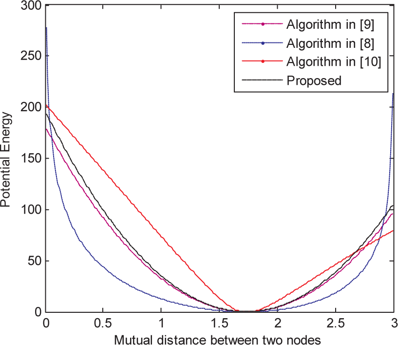
Firstly, we introduce the radial distribution function [24], denoted by g(r), to represents the probability of finding two adjacent nodes separated by a distance r. g(r) is commonly used to measure the translational order of a condensed system, and we adapt it here to the evaluation of the performance of the VFA. In two-dimensional space, it has the form:

g (r) = \frac{S}{N} \frac{N (r, Δ)}{2 π r Δ}

(4)

where S is the area covered by sensor nodes, N is the number of the sensor nodes, and N(r, Δ) denotes the number of nodes locating between r-Δ/2 and r+Δ/2.

Based on the definition of g(r), we further define a radial distance measurement between a network topology and a perfect hexagonal configuration as:

δ_{p c} (Ω, Ω_{H}) = \frac{{\int_{0}^{r_{B}} ‖ g_{Ω} (r) - g_{Ω_{H}} (r) ‖}^{2} d r}{\int_{0}^{r_{B}} {‖ g_{Ω_{H}} (r) ‖}^{2} d r}

(5)

where Ω denotes the resultant network topology, Ω_H denotes the topology of a perfect hexagonal configuration, and r_B is the bound of the radial distance. This distance measurement is called PCD. For a network the topology of which is approximate to a perfect hexagonal configuration, its PCD value should be small. A perfect configuration of a network has a PCD value of zero.

Moreover, the PCD can be applied for characterizing the convergence rate of a VFA. Starting from an initial node distribution, the pair-correlation diversion decreases as deployment progresses over time. When the network converges on a stable structure, the PCD value stabilizes.

4. Spring force algorithm

Inspired by elastic springs with damping in daily life, we introduce a novel VFA called ‘Spring Force Algorithm’ (SFA). F_i^e(t) and F_i^f(t) are specified in the SFA. It is a distributed algorithm in which the force exerted on a node is determined merely by the relative position of its neighbouring nodes. Imagine that a node is connected to its neighbouring nodes by imaginary springs. When the distance between two neighbourhoods is smaller than the original length of the spring – namely, the equilibrium's distance-the spring repels them; when the distance between two neighbourhoods is larger than the equilibrium's distance and within the communication range, the spring draws them closer. The frictional force in the spring system is also called ‘damping’.

4.1 Sensor Movement and Potential Field

Distinct from other algorithms where the formulae of F_i^e(t) and F_i^f(t) are given directly and separately, we analyse the movement of sensors in terms of a differential equation, in which F_i^e(t) and F_i^f(t) are jointly considered. In physics, the differential equation of a sensor node under SFA can be specified as follows:

m \frac{d^{2} x_{i} (t)}{d t^{2}} = - γ \frac{d x_{i} (t)}{d t} - k (x_{i j} (t) - D_{m})

(6)

where k is the elastic coefficient constant of the virtual spring, D _m is a vector with a length of the equilibrium distance and which has the same direction as x _ij(t). The first term on the right side is the viscous frictional force F_i^f(t) and γ is the coefficient of the friction. In the SFA, we can determine the theoretically-optimal friction coefficient and apply it to a network deployment. One of the advantages of SFA is that, instead of using computer simulation or experiment, the theoretically-optimal value of γ can be determined by applying knowledge of vibration in physics.

In a VFA, each node has both potential and kinetic energy: the former arises from the node's interaction with a potential field, the latter from the node's motion [22], Friction has the effect of removing mechanical energy from the system. The total energy will decreases monotonically over time and the total kinetic energy will asymptote to zero. Therefore, the entire system will converge on a static equilibrium.

4.2 Damping Effect

Let k / m = ω₀² and γ / m = 2β. ω₀² be related to the elasticity of the virtual spring. β is relevant to the damping effect and a larger β corresponds to the damping force with greater intensity. When β=0, the virtual spring works in a simple harmonic vibrational state and ω₀ is the vibrational frequency.

We define a new quantity ζ as:

ζ = \frac{γ}{2 \sqrt{k m}}

(7)

Different examples of the damping of spring vibration are depicted in Figure 1 according to Eq. (6). By applying the theory of damped vibration, we know that:

When β<ω₀ and ζ<1, the spring system operates in under-damping condition. The term “under-damping” derives from underdamping vibration of spring in physcis. The damping friction is not sufficient to offset the exchange force in short time and the entire system will experience oscillation for a period of time. The oscillation will cause longer travel distances for the nodes and greater energy consumption, which are undesirable. Moreover, the convergence time is prolonged, which means that more energy is consumed in sensor communication. The smaller that β is, the longer the duration of oscillation will be.

When β>ω₀ and ζ>1, the network system operates in over-damping condition. The frictional force is set so high that the entire system slowly transforms to a condition of equilibrium. As a result, more energy will be wasted on sensor communication. Moreover, the entire system responds slowly to unexpected events and cannot be used for time-critical applications.

When β=ω₀ and ζ=1, the network operates in critical damping condition. The motion is offset by the frictional force and the system will quickly transform to a state of equilibrium without unnecessary vibration or excessive energy usage. Under these circumstances, the value of the parameter γ is theoretically optimal. The relation between k and γ in critical damping condition is:

γ_{c r i t i c a l} = 2 \sqrt{k \cdot m}

(8)

Based on the analysis above, we set β=ω₀ and will apply it to the algorithm's simulation.

Figure 1.

Solution of Eq. (7) under different damping conditions

We restrict the exchange force to only those neighbouring nodes according the rule in [8]. For node i, we denote the set of its neighbouring nodes which could exert force on it as S_i(t). A node k belongs to S_i(t) if it locates within the communication range of node i and there are no other nodes k' shielding the mutual influence between node i and k. Node k' shields k if k' is closer to i and the angle formed by r_ik and r_ik, is smaller than 60°. Shielding plays a crucial role in constructing the regular hexagonal configuration of the network.

A second-order leap-frog scheme was utilized for the numerical solution of the differential equation. Mathematically, it is given by the following formula:

\begin{array}{l} x_{i} (t + 1) = x_{i} (t) + v_{i} (t) d t + \frac{a_{i} (t)}{2} (_{t}^{d)} \\ v_{i} (t + 1) = v_{i} (t) + \frac{(a_{i} (t) + a_{i} (t + 1))}{2} d t \end{array}

(9)

where v_i(t) and a_i(t) are the velocity and acceleration of node i at time slot t, respectively. The virtual force results in acceleration on the sensor nodes. Afterwards, acceleration accumulates to velocity and makes the nodes move.

5. Desirable damping

Frictional force is indispensable for a VFA. In a spring oscillator system, the frictional force is also called the ‘damping force’. Damping has the effect of removing energy from the system and making it converge in static equilibrium. In this section, we will analyse the effect of different damping intensities more specifically. Next, we will discover the optimal damping value or else a desirable damping combination.

5.1 The Fixed Damping Case

Firstly, we assume that the damping value is fixed in the process of sensor deployment. It has been proven that in order to achieve complete coverage while maximizing the network area covered by the given nodes, the distance between two sensor nodes should at least be √3r, i.e., | r_ij | ≥ √3Rs [8]. We set the total number of sensor nodes as 200. The equilibrium distance Dm is 1.732. Next, the sensing range of the sensor node is Dm/√3=1 and the communication range is 3. The elastic coefficient k is set as 20.

Through Eq. (8), we get the result that, under critical damping condition, γ_critical≈8.944. We apply those parameters in the simulation and obtain the PCD, convergence time and travel distance of the deployment process. For comparison, we set γ₁=0.8γ_critical, γ₂=1.5γ_critical and γ₃=2γ_critical, respectively, while the values of the other parameters remain unchanged. Simulation results and performance evaluation are also obtained.

Figures 2(a) and (b) give the initial and final distributions of the SFA in the case of critical damping. The circles around the nodes represent the sensing range Rs of the sensors. The deployment results of uncritical damping are similar to Figure 2(b), so for convenience we do not show them here.

Figure 2.

(a) Initial and (b) final distribution of the SFA in the case of critical damping

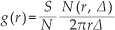
Figure 3 shows, with different damping, the improvement of network configuration from initial deployment in terms of PCD. The four curves exhibit performances of distinct algorithms in terms of uniformity and convergence times, as the deployments progress. We can conclude from this figure that:

When γ=0.8γ_critical, the network deploys in under-damping conditions. The PCD curve vibrates more drastically than the other curves do. A more drastic vibration indicates a greater travel distance and greater energy consumption, which is consistent with the statistics shown in Table 1. In this case, the final PCD value is the lowest among the four cases, so that the final topology is more uniform. However, additional waiting time is required before the network converges.

When γ=1.5γ_critical or 2.0γ_critical, the algorithm works in over-damping conditions. The curves decrease slowly and the final PCD values are higher, which indicates a slower deployment process. However, the average distance travelled by the nodes is shorter and less mobile energy is consumed.

For critical damping, the network topology converges in around 230 steps, which is faster than any other damping case, and the final PCD in this case is 0.4. In this case, the network responds quickly to emergency events. Energy consumption is moderate and the final topology is desirable.

Figure 3.

PCD of the network topology over time under different damping conditions

Table 1.

Average movement distance of the sensors under different damping conditions

γ Value	Average Travel Distance
γ_critical (critical damping)	11.55
γ₁ =0.8γ_critical	20.55
γ₂ =1.5γ_critical	7.16
γ₃ =2.0γ_critical	5.81

If we take all the performance indicators into consideration-including the convergence time, travel distance and uniformity-critical damping is desirable for the SFA.

5.2 The Dynamic Damping Case

In Section 5.1, the damping value remains constant during sensor deployments. In this subsection, we assume that the damping coefficient is dynamic and that it varies in different stages of deployment process. Each damping condition, with its unique characteristic, should play to its strengths in different deployment stages.

From Figure 3, we know that significant damping has the advantage of a faster convergence speed during the early stages and less vibration (lower energy consumption for moving sensors), while it has the disadvantage of a longer total convergence time (higher energy consumption for sensor communication) and worse topological uniformity. In contrast, a low level of damping has the advantage of better resultant topological uniformity, but has the disadvantage of serious early-stage chaos and more vibration.

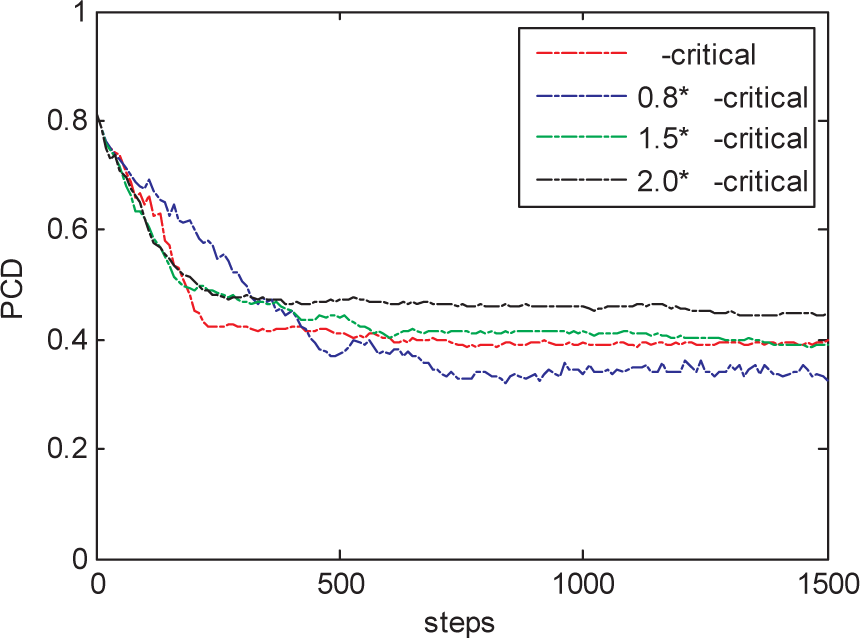
Based on the analysis above, we design a damping-switch scheme. During the early stages (0~250steps) of deployment, γ=1.1γ_critical>γ_critical, the network quickly converges on a desirable configuration; during the middle stages (251~700steps), γ=0.82γ_critical<γ_critical, the virtual energy slowly dissipates and deployment proceeds with minute adjustments; during the final stages (701~1500steps), γ=γ_critical, the entire system converges on a static equilibrium.

Figure 4.

PCD of dynamic damping compared with that of fixed damping

6. Comparison of simulation results

In this section, we verify the effectiveness of the proposed approach through the comparison of the simulation results. A binary detection model [5] is used here. A second-order leap-frog scheme was utilized for the computational solution of the differential equation. Firstly, we show some results of the deployment of sensor nodes under different VFAs in indoor examples, and we then use the coverage promotion over time to analyse the performance of different algorithms. Secondly, we compare the simulation results of SFA in outdoor cases with those of other algorithms, using the PCD for evaluation. In a critical-damping situation, more energy is saved, the topology converges quickly and a uniform configuration is achieved. We assume that the nodes will not run out of power during the deployment period. Nodes are randomly put into the target area and are guided by the virtual force.

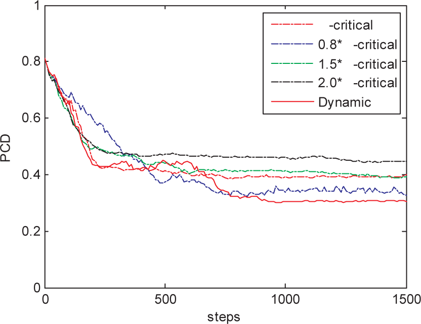
The simulation of the proposed approach in each case of the scenario is compared with that for [8 –10]. Figure 5, below, indicates how the potential energy varies with respect to the mutual distance between two neighbouring sensors for the four algorithms. The position where the potential energy diminishes to zero is the point of equilibrium. The distance between this point and the origin is Dm.

Figure 5.

Potential energy between two adjacent sensors with respect to mutual distance

6.1 The Indoor Case

In an indoor area-there are boundaries surrounding the area-the nodes are initially distributed randomly. The values of the equilibrium distance, sensing range and communication range are the same as for those in the previous section. However, we set an elastic coefficient value from 20 to 15. By referring to [5], we get:

D m^{2} = \frac{1}{ρ_{m} \sin 60^{\circ}} = \frac{S}{N \sin 60^{\circ}}

(10)

Because Dm=1.732 and N=200, we get S=520 while the length of the square side should be 22.8. However, due to the bound effect, we adjust the side length to 22.0 for simulation. Since we are not concerned with the effect of node mass here, we set it to 1 to all nodes for convenience. For the other algorithms being compared, we determine γ through repeated computer simulation tests.

Figure 6(a) and Figure 6(b) depict the random initial distribution and final distribution, respectively. Figure 6(c) plots the coverage variation over time under different algorithms, which shows that the SFA has a better coverage rate than the other algorithms.

Figure 6.

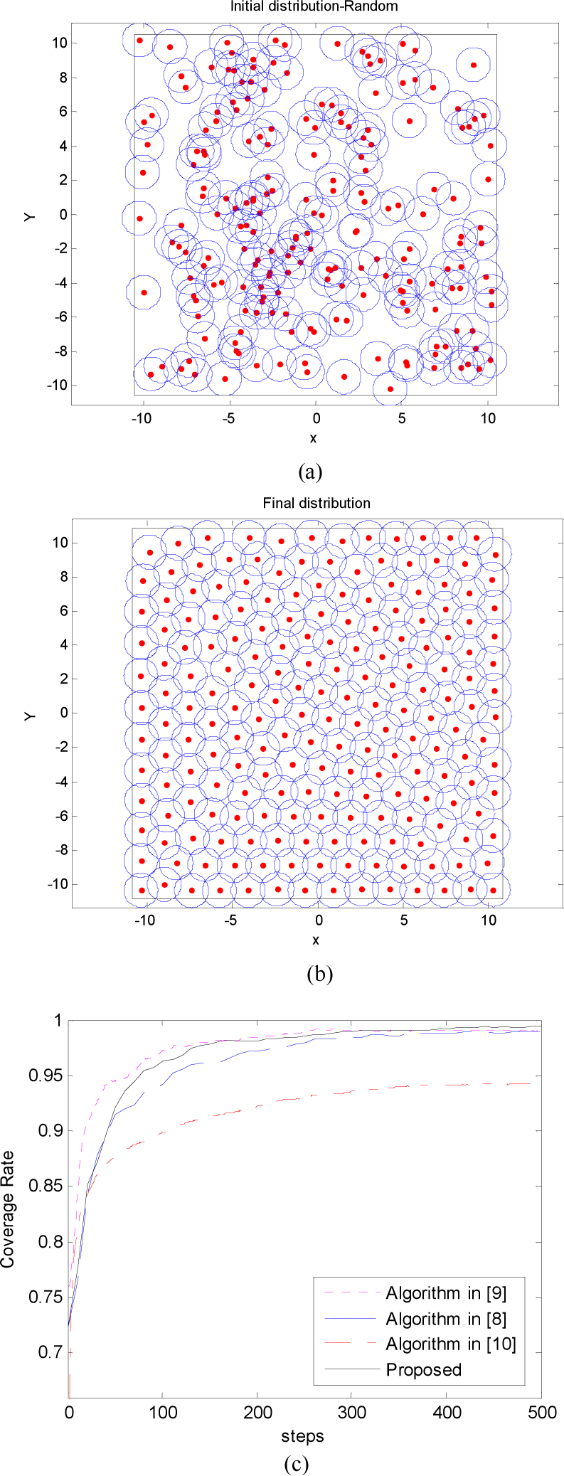
Simulation Results for the ideal indoor case: (a) random initial, (b) final distribution, (c) coverage rate comparison

In order to verify the effectiveness of the proposed algorithm in the more general case, an obstacle is placed in the area of interest. The simulation results are shown in Figure 7. Figures 7(b) and 7(c) show that the proposed algorithm works well for the initial distribution in Figure 7(a) and has better performance.

Figure 7.

Simulation results for the ideal indoor case: (a) random initial, (b) final distribution, (c) coverage rate comparison, (d) enlarged version of (c)

6.2 The Outdoor Case

We also performed simulations for open-area cases-the values of the parameters are the same as those in the indoor case. Figure 8 gives the initial and final distributions of the different algorithms. The average standard deviation of the distance between adjacent nodes for our proposed algorithm is 0.276 while for [8] it is 0.28, which indicates better uniformity in the proposed algorithm.

Figure 8.

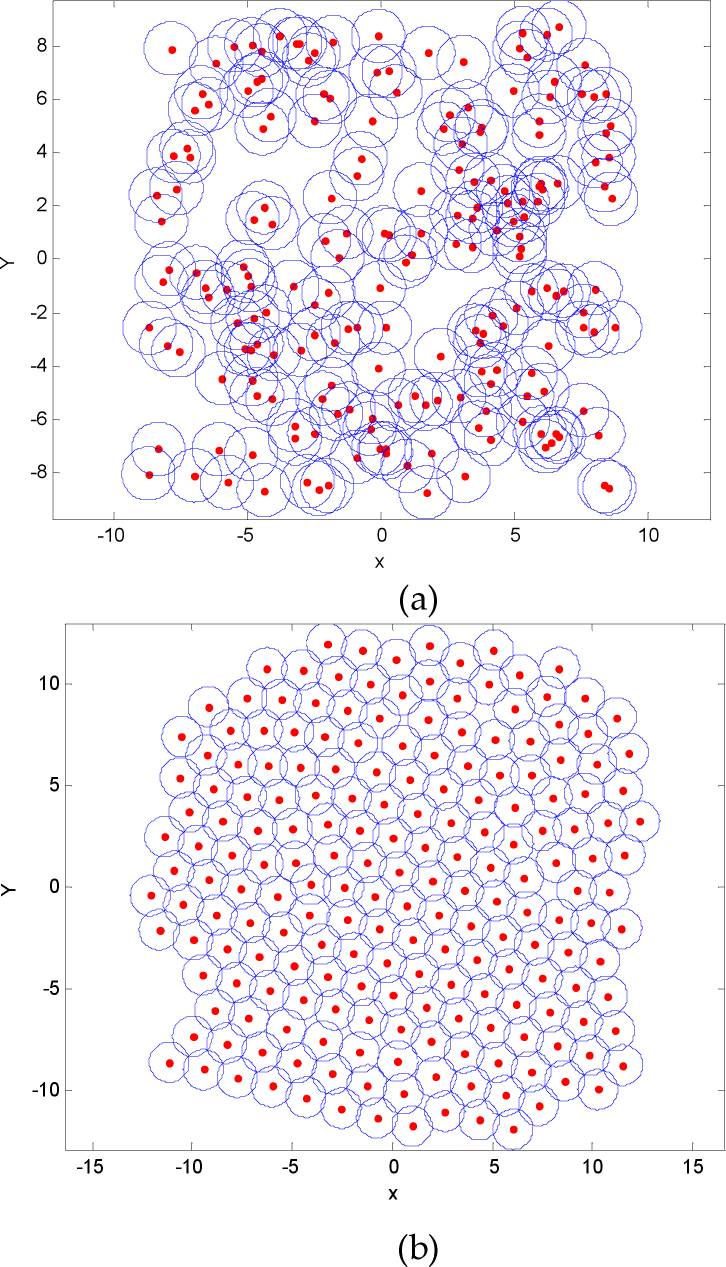
(a) Initial random distribution, (b) final distribution for the proposed approach for the ideal outdoor case

Figure 9 depicts the pair correlation [26] of the network topology under different algorithms. Through the comparison of the pair correlation, we are informed of the proximity between deployment result under each algorithm and the perfect hexagonal network, which indicates that the deployment under the proposed algorithm has the advantage of closer resemblance to a perfect hexagonal network.

Figure 9.

Comparison of the pair correlation of different deployment algorithms

Figure 10 depicts the improvement of the network's uniformity through the process of deployment. The curves of the proposed algorithms reach 0.32 in the end, which is superior to other approaches. Since the value of elastic coefficient manually set here is smaller than that in the previous subsection, the convergence speed of the spring force in Figure 10 is slower than in Section 5.

Figure 10.

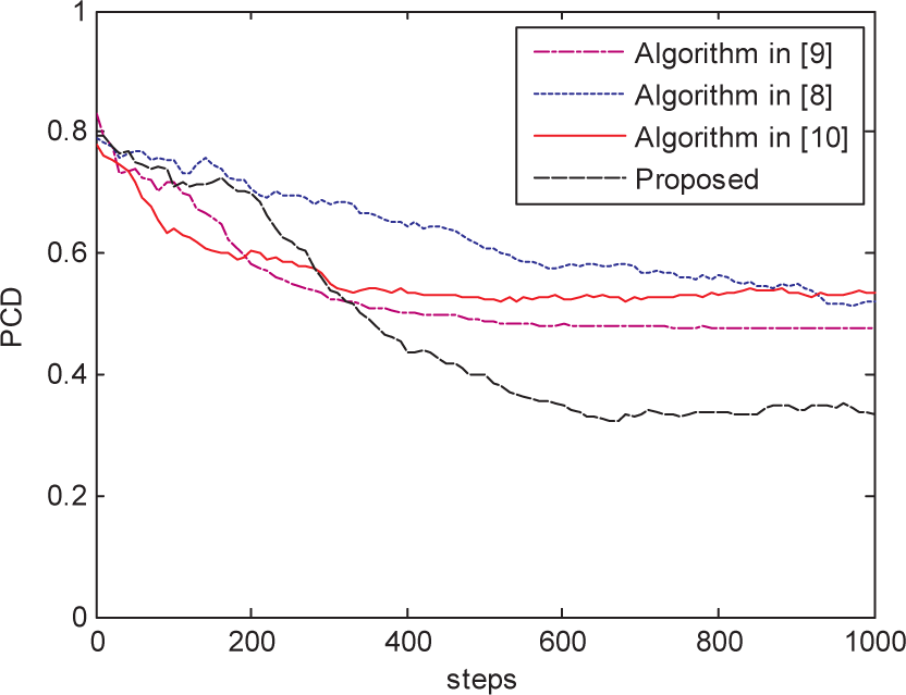
PCD promotion over time under different algorithms

Figure 11 simulates the case in which sensors are dropped by an airplane over an open area. Sensors initially lie almost in a straight line, and they deploy themselves in a better topology. The standard deviation of the distance between adjacent nodes for the proposed approach is 0.301 while for [8] is 0.317, which also means better uniformity in the proposed algorithm. The PCD improvement comparison in Figure 11(d) also illustrates this point. The curves of the proposed algorithms decline more significantly than for that of the algorithm in [8], although this distinction is not visually detectable in Figures 11(b) and 11(c).

Figure 11.

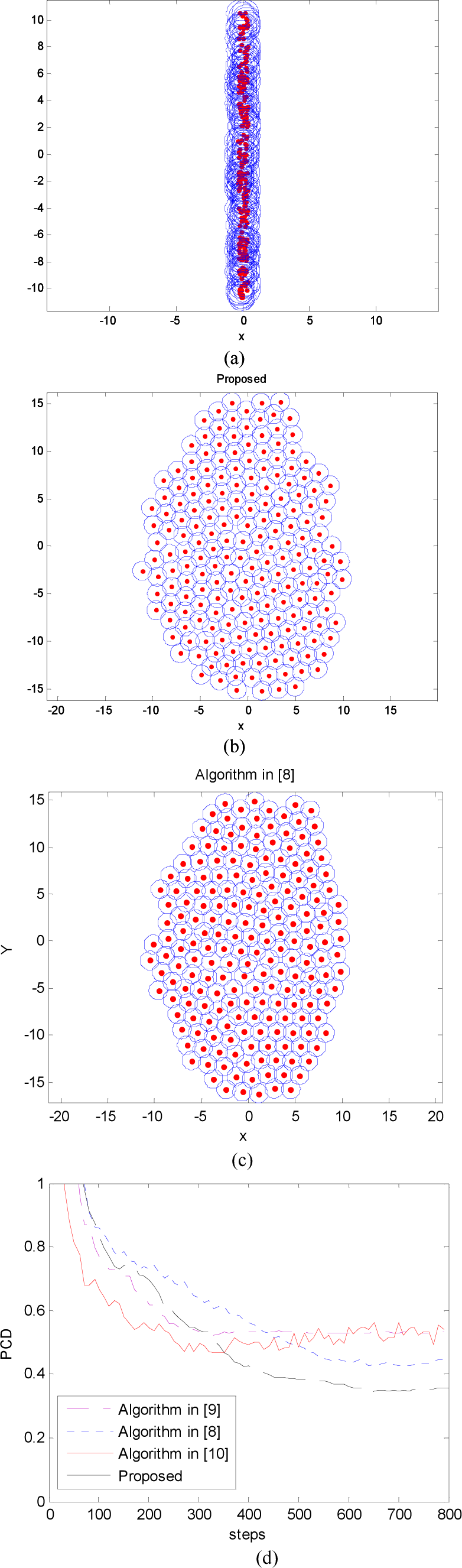
(a) Initial random distribution, final distribution for (b) final distribution for the proposed algorithm, (c) final distribution for algorithm in [8] and (d) PCD promotion over time under different algorithms

7. Conclusions

In this paper, a virtual force-based sensor deployment algorithm using a spring force model is proposed and a shielding rule that restricts the number of neighbours exerting force is adapted. A new metric called ‘pair correlation’ is introduced to evaluate the uniformity of the nodes' distribution. The simulation results indicate how proper damping conditions promote the algorithm's performance in terms of convergence time, coverage rate, topological uniformity and energy consumption. With the SFA, the amplitude of exchange force is linearly proportional to the distance between neighbouring nodes. In other algorithms, the exchange force may be nonlinear, but a similar damping selection method can be applied and further research is required. Irregular terrains and more complex situations will be considered in our future work.

Footnotes

8. Acknowledgements

This work was supported by the Foundation for National Natural Science Foundation of China (Grant No. 61201178), the Fundamental Research Funds for the Central Universities (Grant No. 2014ZZ0039), Distinguished Young Talents in Higher Education Guangdong China (Grant No. LYM10011), Scientific Project of Guangdong (No. 2010B010600019) and United Foundation Project of Guiyang University Guizhou (Grant No. QianKeHeJ-LKG[2013]36).

References

Zheng

Jamalipour

(2009) Wireless sensor networks: a network perspective. IEEE Press, NJ, 2009. p. 466.

Akyildiz

I.F

Sankarasubramaniam

Cayirci

(2002) Wireless sensor networks: a survey. Computer Networks. 38: 93–422.

Chen

Shen

Sun

(2009) The deployment algorithms in wireless sensor net works: a survey. Information Technology Journal. 8: 293–301.

Younis

Akkaya

(2008) Strategies and techniques for node placement in wireless sensor networks: a survey. Ad Hoc Networks. 6: 621–655.

Zou

Chakrabarty

(2003) Sensor deployment and target localization based on virtual forces. Proceedings of the IEEE INFOCOM. New York, USA: 1293–1303.

Heo

Varshney

P.K

(2005) Energy-efficient deployment of intelligent mobile sensor networks. IEEE Transactions on Systems, Man, and Cybernetics-Part A: Systems and Humans. 35: 78–92.

Kribi

Minet

Laouiti

(2009) Redeploying mobile wireless sensor networks with virtual forces. Wireless Days (WD), 2009 2nd IFIP: pp. 1–6.

Garetto

Gribaudo

Chiasserini

C.F

Leonardi

(2007) A distributed sensor relocation scheme for environmental control. IEEE International Conference on Mobile Ad-hoc and Sensor Systems (MASS): 1–10.

Huang

Lan

Qian

(2012) A novel virtual force approach for node deployment in wireless sensor network. Proceedings of IEEE International Conference on Distributed Computing in Sensor Systems, DCOSS 2012, Hangzhou, China: 359–363.

10.

Huang

Lan

Qian

(2012). A van der Waals force-like node deployment algorithm for wireless sensor network. Proceedings of the 8th International Conference on Mobile Ad-hoc and Sensor Networks, Chengdu, China: 218–221.

11.

Chen

Sun

(2007) Novel deployment schemes for mobile sensor networks. Sensors. 7: 2907–2919.

12.

Pan

(2005) Sensor deployment optimization for detecting manoeuvring targets. Information Fusion 2005, Philadelphia, PA, USA: 1629–1635.

13.

Zhang

B.H

Cui

L.G

Chai

S.C

(2012) An extended virtual force-based approach to distributed self-deployment in mobile sensor networks. International Journal of Distributed Sensor Networks. 2012, Article ID 417307, p. 14.

14.

Kukunuru

Thella

Davuluri

(2010) Sensor deployment using particle swarm optimization. International Journal of Engineering Science and Technology. 2: 5395–5401.

15.

Lei

(2009) Sensor node deployment in wireless sensor networks based on improved particle swarm optimization. In Proceedings of 2009 IEEE International Conference on Applied Super-conductivity and Electromagnetic Devices, Chengdu, China: 215–217.

16.

Liao

Kao

(2011) A sensor deployment approach using glowworm swarm optimization algorithm in wireless sensor networks. Expert Systems with Applications. 38: 12180–12188.

17.

Ozturk

Karaboga

Gorkemli

(2012) Artificial bee colony algorithm for dynamic deployment of wireless sensor networks. Lurk. J. Elec. Eng. and Comp. Sci. 20: 255–262.

18.

Ozturk

Karaboga

Gorkemli

(2011) Probabilistic dynamic deployment of wireless sensor networks by artificial bee colony algorithm. Sensors. 11: 6056–6065.sd.

19.

Wang

Cao

Porta

(2006) Movement-assisted sensor deployment. IEEE Transactions on Mobile Computing. 5: 640–652.

20.

Wang

J.J

(2007) An improved co-evolutionary particle swarm optimization for wireless sensor networks with dynamic deployment. Sensors. 7: 354–370.

21.

Han

Kim

Jeong

(2012) An energy-efficient self-deployment with the centroid-directed virtual force in mobile sensor networks. Simulation. 88: 1152–1165.

22.

Howard

Mataric

M.J

Sukhatme

G.S

(2002) Mobile sensor network deployment using potential fields: a distributed, scalable solution to the area coverage problem. Proceedings of the 6th International Conference on Distributed Autonomous Robotic Systems. Fukuoka: 299–308.

23.

Poduri

Sukhatme

G.S

(2004) Constrained coverage in mobile sensor networks. Proceedings of the IEEE International Conference on Robotics and Automation (ICRA). Los Angeles, CA: 40–50.

24.

Hua

J-J

Liu

Y-H

M-F

Wang

Zhang

Z-H

(2003) Structural and dynamical analysis of a two-dimensional dusty plasma lattice, Chinese Physics Letters. 20:155–157.

25.

Quinn

Cui

Goree

Pieper

J.B

Thomas

Morfill

G.E

(1996) Structural analysis of a Coulumb lattice in a dusty plasma. Phys. Rev. E. Stat. Phys. Plasmas Fluids Relat. Interdiscip. Topics. 53: 2049–2052.

26.

Wen

Qian

Song

Bartos

(2014) On virtual-force algorithms for coverage-optimal node deployment in mobile sensor networks. Unpublished work.

A Deployment Method Based on Spring Force in Wireless Robot Sensor Networks

Abstract

Keywords

1. Introduction

2. VFAs

2.1 Review of VFAs

2.2 Sensor Movement of the VFA

3. Evaluation of the VFA's performance

3.1 Convergence Time

3.2 Moving Distance

3.3 Coverage

3.4 Uniformity

4. Spring force algorithm

4.1 Sensor Movement and Potential Field

4.2 Damping Effect

5. Desirable damping

5.1 The Fixed Damping Case

5.2 The Dynamic Damping Case

6. Comparison of simulation results

6.1 The Indoor Case

6.2 The Outdoor Case

7. Conclusions

Footnotes

8. Acknowledgements

References