
Abstract
Reliable dissemination of bulk data is one of the important problems in sensor networks. For
example, programming or upgrading the software in sensors at run-time requires reliable
dissemination of a new program across the network. In this paper, we present
Infuse, a time division multiple access (TDMA) based reliable data dissemination
protocol. Infuse takes two input parameters: the choice of the recovery algorithm (from one of two presented in this paper) to deal with
unexpected channel errors (e.g., message corruption, varying signal strength), and whether a sensor should listen only to a subset of its neighbors to reduce the amount of active
radio time.
Based on these parameters, we obtain four possible versions of Infuse. We compare the performance of these versions to assist a designer in selecting the appropriate version based on the network characteristics. Furthermore, we demonstrate Infuse in the context of network programming.
Keywords
Introduction
Sensor networks have become popular due to their application in unattended tracking and detection
of undesirable objects, hazard detection, data gathering, environment monitoring, and so on.
Furthermore, due to their low cost and small size, it is easy to deploy them in large numbers.
Reliable dissemination of bulk data is one of the important problems in such networks. For example,
in sensor networks, reprogramming the sensors in place is often necessary since the
sensors are deployed in large numbers and in inaccessible fields. Moreover, the requirements of a
typical sensor network application (e.g., A Line in the Sand [1,2]) evolve over time and, hence, reprogramming or upgrading the software in the sensors
after deployment is necessary. Especially in the context of reprogramming, the problem of reliable
data dissemination has been studied in two main scenarios: reprogramming of sensors in a laboratory environment prior to deployment, and reprogramming of sensors in the field after deployment.
In this paper, we focus on the latter scenario.
Challenges in reliable data dissemination
One of the important challenges in reliable dissemination of bulk data is that the network is multishop in nature. The communication range of the sensors is limited and, hence, they need to collaborate with each other to forward the data across the network. As a result, approaches such as XNP [3], where the sensors are assumed to be within the communication range of the base station, are not suitable.
Another challenge in sensor networks is the nature of message communication. Specifically, the basic mode of communication in sensor networks is local broadcast with collision. In other words, when a sensor communicates, it can update the state of its neighboring sensors. However, if multiple messages are sent to a sensor simultaneously then, due to collision, it receives none. This can also occur due to the hidden terminal effect, where a given message may collide at one sensor and be correctly received at other sensors.
To provide reliable message communication, different medium access control (MAC) protocols are proposed for sensor networks. Collision-avoidance protocol like carrier-sense multiple access (CSMA) offers only probabilistic guarantees about message communication. Most of the existing solutions for multihop data dissemination (e.g., [4–9]) use CSMA and, hence, rely on other mechanisms such as acknowledgments/negative-acknowledgments, advertisements/request schemes, and/or error correcting codes.
Collision-free MAC protocol like time division multiple access (TDMA) offers deterministic guarantees about message communication and, hence, it is desirable for reliable data dissemination. Other collision-free protocols include frequency division multiple access (FDMA) and code division multiple access (CDMA). FDMA is often used with TDMA where each sensor knows when to listen to a particular frequency. CDMA requires special hardware for encoding/decoding messages and, hence, it is not desirable for resource poor sensors.
Contributions of the paper
With this background, in this paper, we propose Infuse,
1
a TDMA based data dissemination protocol for sensor
networks. Infuse can be used with any TDMA protocol (e.g., [10–12]). The main contributions
of the paper are as follows: We present Infuse a TDMA based reliable data dissemination protocol. Although
TDMA guarantees collision-free communication, in the presence of channel errors (e.g., message
corruption, varying signal strengths), random message losses occur during dissemination. To deal
with this problem, we consider two recovery algorithms based on the sliding window protocols [17, 14]. Specifically, we extend an instance of the sliding window
protocol from [13] where we use
implicit acknowledgments (received by listening to the transmissions of the
successors of a sensor) and messages that provide acknowledgments for several previous messages. We show that the active radio time during dissemination is significantly less than the latency.
We also present a simple heuristic to reduce the active radio time further. With this approach, a
sensor typically receives new messages from only one sensor. Moreover, we show that the active radio
time during dissemination is significantly less than that of the approaches proposed in [17, 9]. We verify that Infuse propagates data in a pipelined fashion. Also, we show that it does not have
the behavior expressed in Deluge [7],
where sensors along the edge of the network receive the data first before the diagonal. We also
implement Infuse in TinyOS [15] for
Mica-2 [16] and XSM [17] mote platforms.
Organization of the paper
In Section 2, we present the protocol and in Section 3, we discuss its properties. Then, in Section 4, we present the simulation results. In Section 5, we compare Infuse with other solutions. Subsequently, in Section 6, we show Infuse can be used in the context of network programming. Finally, in Section 7, we discuss some of the questions raised by this work and in Section 8, we make concluding remarks.
Infuse: Data Dissemination Protocol
In this section, first, we present the protocol architecture of Infuse. We assume that there is a base station that is responsible for communicating with the outside world. The base station initiates the bulk data transfer whenever it receives a startDissemination message from the outside world (e.g., the monitoring/visualization station in the Line in the Sand experiments [17, 2]). The data is split into fixed size packets called capsules. The start Dissemination message includes the ID of the new data and the number of capsules. Additionally, it may include the location (in EEPROM) where the sensors should store this data. Note that Infuse is not concerned with the contents of the data. For example, in difference-based reprogramming [18], the data is the difference between the old and the new programs. Moreover, the data could be encrypted (e.g., using link-layer encryption mechanism like TinySec [19]) to prevent malicious reprogramming or dissemination. Upon receiving the startDissemination message, the base station sends the startDownload message (that includes the ID of the new data, number of capsules, and optionally, the location where the sensors should store the data) to all its neighbors; these neighbors, in turn, forward it to their neighbors. Whenever a sensor receives the message, it initializes appropriate data structures in order to store the new data. Furthermore, it signals the application that a download is in progress. And, when the sensor receives the complete data, it signals the application that the download is complete. Figure 1 shows the Infuse protocol architecture.

Infuse protocol architecture.
TDMA Service
The dissemination layer relies on a TDMA service (e.g., [10–12]) that may in turn use a localization service (e.g., [20]). The TDMA service identifies the slots in which a sensor can transmit and the slots in which it should listen to its neighbors. We assume that the TDMA service provides a fair share of bandwidth to each sensor. One way to achieve this is to ensure that between every two slots assigned to a sensor, at least one slot is assigned to its neighbors. Also, we assume that the slots assigned to the sensors are periodically revalidated to deal with transient errors and/or clock drift. In Section 2.3, we recall the TDMA algorithm from [10] as an example that could be used with Infuse.
Ideal scenario
Once the base station sends the startDownload message, in its subsequent TDMA slots, it sends
data messages. Each message contains a capsule, say c
l
, its sequence
number, say n
l
, and information for providing recovery (cf. Section 2.1). Whenever a sensor receives a
capsule (say, c), it stores c at the appropriate location and enqueues it in the TDMA queue; thus, c
will be forwarded to additional sensors farther from the base station. Infuse takes two (compile
time) parameters: the choice of recovery algorithm, and whether a sensor should listen to only a subset of its neighbors to reduce active radio time (at
the cost of increasing the latency).
We describe the role of these parameters, next.
Parameter 1: Recovery algorithm. Although TDMA guarantees collision-freedom, background noise can cause random message losses. While dealing with these problems, the padding added to a message should be minimized since the payload size of a message is often limited (e.g., 29 bytes in Mica motes [16]). Also, the preamble added to a message in the lower layers of communication stack is high (e.g., 20 bytes in Mica). Hence, unnecessary communication (in terms of explicit acknowledgments) needs to be avoided.
During dissemination, whenever the successors of a sensor (say, j) forward the capsule (say, c), j gets an implicit acknowledgment for c. We use this information to recover from lost capsules. We compare two recovery algorithms based on the sliding window protocols [13,14]. The recovery algorithms use implicit acknowledgments unlike the explicit acknowledgments used in the traditional sliding window protocols. The first algorithm, Go-back-N (cf. Section 2.1.1), does not add any padding to a message. The second algorithm, selective retransmission (cf. Section 2.1.2), adds 2b bits to a message, where 2b is the size of the window.
Parameter 2: Selective listening to neighbors. In the context of bulk data dissemination, a sensor may receive a message several times, once from each of its neighbors. To reduce duplicate messages, it is desirable that a sensor listens to only a subset of its neighbors. However, in this case, the latency may increase since the duplicate messages may assist in dealing with random message losses. When such selective listening is desired, each sensor classifies its neighbors as predecessors and successors. Initially, all neighbors are (potential) predecessors as well as (potential) successors. Now, given two neighbors j and k, if k forwards a majority of new packets before j then j marks k as its predecessor (i.e., removes k from successor list) and k marks j as its successor (i.e., removes j from predecessor list). Once a sensor classifies its neighbors, it can choose to listen to 1 or more predecessors (for new capsules) and 0 or more successors (for implicit acknowledgments and recovery). (Note that when selective listening is not desired, all neighbors are treated as potential predecessors and successors.)
Based on these parameters, we obtain four possible versions of Infuse. Note that the version is selected at compile time, i.e., all sensors will be running the same version in any given experiment. In Section 4, we compare these versions to assist a designer in selecting the appropriate version based on the network characteristics. We describe the details of these versions, next.
In our protocol, each sensor transmits a capsule in its TDMA slot. In order to deal with channel errors, in this section, we consider two recovery algorithms; these algorithms identify the capsule a sensor should forward in its TDMA slot. This is unlike CSMA based dissemination protocols (e.g., Deluge [7], MNP [9]) where extra steps (e.g., mechanism to reduce concurrent senders, transmitting meta-data about the availability of new data using advertisements, etc) need to be taken to prevent congestion and reduce collisions. Since there is no collision with TDMA, there is no need for elaborate control and each sensor can independently decide what capsule to send in its TDMA slot.
Go-Back-N Based Recovery Algorithm
In this algorithm, a sensor transmits a capsule with sequence number nf if it has received all capsules with sequence number smaller or equal to n f . Thus when a sensor transmits a capsule with sequence number nf, it provides implicit acknowledgment for all capsules 0,…,nf. To provide recovery in the presence of channel errors, each sensor maintains (in RAM) a window of capsules with sequence number nia −1,…,nia + 2 b, where nia is the highest sequence number for which the sensor has received an implicit acknowledgment from all its successors and 2b is the size of the window. Note that some of the window locations may be empty, if the corresponding capsules are not yet received. When a sensor receives a capsule in this window, it stores the capsule both in its RAM and EEPROM. Now, a sensor (say, j) will forward capsule cf(with sequence number nf) only when all its neighbors have forwarded capsules with sequence number nf − b or higher (i.e., nia ≥ nf − b). Otherwise, j will start retransmitting its current window, i.e., it will transmit the capsule with sequence number n ia + 1. This creates a back pressure in the network and, hence, the rate of dissemination of new capsules is reduced during recovery (cf. Fig. 2 for the algorithm).

Implicit acknowledgments and Go-back-N algorithm.
As an illustration, consider the data dissemination process shown in Fig. 3, where the window size is 2. In Fig. 3(i), sensors transmit capsules 10,9,7,6 in time slots s1, s2, s3, s4, s1 < s2> s3 < s4, respectively. In Fig. 3(ii), the second sensor forwards capsule 8 in slot s2 + P, where P is the period between successive TDMA slots. This is due to the fact that the second sensor did not receive implicit acknowledgment for capsule 8 from its successor. Hence, instead of forwarding capsule 10, it goes back and starts retransmitting from capsule 8. Similarly, in Fig. 3(iii), the first sensor forwards capsule 10 instead of 12. Thus, lost capsules are recovered.
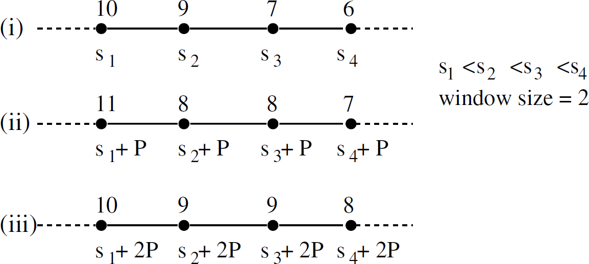
Illustration of Go-back-N algorithm on a linear topology.
Dealing with failed sensors. In the presence of failed sensors, neighboring sensors will not get implicit acknowledgments. To deal with this problem, whenever a sensor fails to get an implicit acknowledgment from its successors after a fixed number of retransmissions, it declares that neighbor as failed. Now, a sensor will retransmit a capsule only when it does not receive an implicit acknowledgment from its active neighbors.
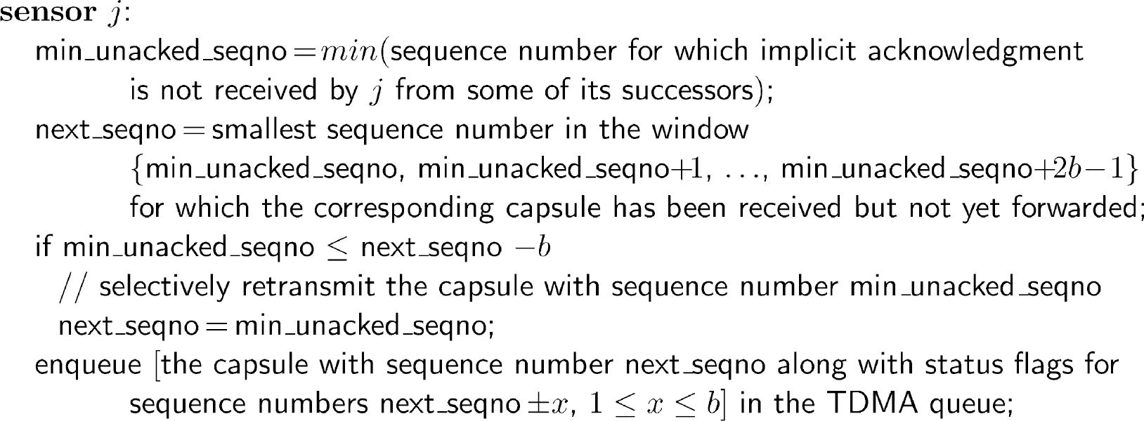
Similar to Go-back-N, in this approach, each sensor maintains a window of 2b capsules, where b is any integer. However, unlike Go-back-N, a sensor (say j) will transmit the capsule with sequence number nf even if it has not received some capsules with sequence number smaller than nf. (This can happen due to channel errors.) Rather, j transmits capsule with sequence number nf only if it has received all capsules with sequence number 0,…,nf−b−1. Also, the sensor piggybacks acknowledgments for capsules with sequence number nf−b,…,nf—1, nf+1,…,nf+b. The piggybacked acknowledgments are used by its predecessors to determine the highest sequence number for which acknowledgment is not yet received (nunacked) from some neighbor. To recover from lost capsules, j will forward capsule cf (with sequence number nf) only if nunacked > (nf − b). Otherwise, j will retransmit the capsule containing the sequence number nunacked. After retransmission, j will try to forward capsule with sequence number nf in its next TDMA slot. The intuition behind selective retransmission is that even if a sensor misses a capsule transmitted by one of its predecessors, it may still receive the capsule from other neighbors. (This is due to the fact the sensors may have more than one path to the base station.) Furthermore, the piggybacked acknowledgments update the predecessors about the missing capsules at the successors. This also allows the predecessors to listen infrequently to the implicit acknowledgment of successors. Thus, it can be used to reduce message communication and active radio time (cf. Fig. 4 for the algorithm).
Implicit acknowledgments and selective retransmission.
As an illustration, consider the data dissemination process in Fig. 5, where the window size is 2. Each sensor is shown transmitting c [m|n], where c is the actual capsule forwarded by the sensor, m and n are the piggybacked acknowledgments for capsules c − 1 and c + 1 respectively. If m (respectively, n) is c − 1 (respectively, c + 1), the predecessors get an implicit acknowledgment for the corresponding capsule. If m or n is represented as “X”, it indicates that the sensor is yet to receive that capsule. In Fig. 5(i), sensors forward capsules 10, 9, 7, 6 in time slots s1, s2, s3, s4, s1 < s2 < s3 < s4 respectively. The second sensor missed capsule 10 due to channel errors and it forwards 9[8|X] in slot s2. Since the window size is 2 (i.e., b=1), the first sensor cannot forward capsule 11 in slot s1 + P, where P is the period between successive TDMA slots. Hence, the first sensor retransmits capsule 10 (cf. Fig. 5(ii)). Similarly, the second sensor forwards capsule 9 in slot s2 + P and s2 + 2P (cf. Fig. 5(ii-iii)). Thus, lost capsules are recovered through selective retransmissions.

Illustration of selective retransmission based recovery algorithm on a linear topology.
Remark. In the presence of failed sensors, the modifications proposed for Go-back-N algorithm (cf. Section 2.1.1) can be applied for this approach as well. Also, we can make the recovery algorithms proposed in this section self-stabilizing using the framework for one-too-many sliding window protocol presented in [13].
As discussed earlier in this section, a sensor (say, j) classifies its neighbors as its predecessors and successors. Then, j selects one of the predecessors as the preferred predecessor. Note that the choice of preferred predecessor of one sensor is independent of that of others. This preferred predecessor is responsible for listening to implicit acknowledgments and recovering lost capsules at j. Now, whenever j forwards a capsule, it includes its preferred predecessor in the message. This can be achieved by log(q + 1) bits, where q is the number of neighbors that a sensor has (and the + 1 term is for the case where preferred predecessor is not yet chosen). Since the predecessors listen to the transmissions of their successors (to deal with channel errors), they learn about the sensors for whom they are the preferred predecessors. Once the preferred predecessor information is known, a sensor (say, k) will listen to the transmissions of j only if j's preferred predecessor is k. Otherwise, k will not listen in the time slots assigned to j. Thus, during data dissemination, the number of message receptions is reduced by allowing only the preferred predecessors to recover lost capsules at their successors.
However, if the preferred predecessor of j fails, j cannot recover from lost capsules. Towards this end, other predecessors will listen to the transmissions of their successors occasionally. In other words, a sensor (say, l) will listen in the time slots assigned to j with a small probability, if 1 is not the preferred predecessor of j. This will allow the successors to change their preferred predecessors and recover from lost capsules.
Remark. We note that the number of messages can be reduced even further as follows. If k is the preferred predecessor of j, k can choose to listen in the time slots assigned to j with a certain probability. This will allow k to listen to the transmissions of j occasionally. However, this is sufficient to recover lost capsules at j, since k learns about the lost capsules at j with the help of the implicit acknowledgments.
SS-TDMA: Broadcast Algorithm
In this section, we recall (from [10]) the self-stabilizing TDMA (SS-TDMA) service customized for broadcast. This service is
based on the radio model from [17, 22], where the authors have evaluated the
signal-to-noise ratio (SNR) of a given message based on the distance between the sending and the
receiving (Mica) sensors. Specifically, in [17, 22], the authors show that
up to a certain distance (communication range) the messages are received almost
with certainty. Also, after a certain distance (interference range), the message
reception is close to 0 and SNR is very low and, hence, the message is unlikely to
interferencerange affect any other communication. They also show that the value of
The protocol in [10] uses this communication range and interference range to assign timeslots for sensors arranged in a grid, where the base station is in top-left (north-west) corner (at location <0, 0>). They assume that for any sensor its neighboring sensors in the grid are within communication range and the sensors up to Manhattan distance of y hops are in the interference range, where y is called the interference ratio. For such a network, they show that if the sensor located at location (i, j) transmits at slot i + (y + 1) j + c∗ ((y + 1) 2 + 1), c ≥ 0, then the communication is collision free. Of these, i + (y + 1) j is the initial slot for the sensor whereas ((y + 1)2 − 1) is the period (P) between two slots assigned to a sensor. Based on the results from [17, 22], we use y = 4 in most of the simulations. For dense networks, where y is larger, we discuss the results in Section 7.
Note that in [10], the authors also present approaches for initial slot assignment and slot validation to deal with transient errors and/or clock drift. These issues are not relevant in this context and, hence, are not discussed here. Furthermore, Infuse does not depend on this algorithm; we only use this algorithm to illustrate (most of the) simulation results for Infuse, as the protocol from [10] is applicable in [2]. Other TDMA algorithms (e.g., [11]) can also be used with Infuse (cf. Section 4.6). The reader need not be familiar with these TDMA algorithms; it suffices for them to assume that the TDMA algorithm assigns slots in such a way that a sensor can communicate with its neighbors in a collision-free manner.
Infuse: Properties
In this section, first, we discuss how the data is propagated in a pipeline and estimate the latency in presence of no channel errors. Next, we argue that our approach is energy-efficient.
Pipelining
In Infuse, whenever a sensor receives a capsule, it stores the capsule in the flase at the appropriate address. Then, it forwards the capsule in the next TDMA slot. Hence, the capsules are forwarded in a pipeline fashion. If P is the period between successive TDMA slots, it takes at most d ∗ P time to forward one capsule across the network, where d is the diameter of the network (= 2(n − 1), in case of n × n grid network). If ctot is the number of capsules in the data, as a result of pipelining, once the first capsule is forwarded, the remaining capsules can be forwarded within (ctot − 1) ∗ P time. Thus, in the presence of no channel errors, the time required to disseminate data with ctot capsules is ((ctot − 1) + d) ∗ P. This provides an analytical estimate for the dissemination latency. For bulk data, ctot ≫ d. Therefore, dissemination latency is independent of the network size.
Energy-efficiency
In Infuse, the energy spent during dissemination is equal to the sum of energy spent in idle-listening, message receptions, message transmissions, and writing to EEPROM or external flash.
Since all the sensors are required to write the data to their external flash, the energy spent in writing to external flash is a constant across the network. Additionally, in Infuse, each sensor forwards every capsule at least once. Hence, the number of message transmissions remains almost a constant across the network. Finally, in most sensor network platforms (e.g., Mica-2 [16]), the energy spent in idle-listening is equal to the energy-spent in receiving a message. Therefore, the energy spent during dissemination is determined by the amount of active radio time.
With TDMA, a sensor remains in active mode only in its TDMA slots (if it needs to send any capsule) and in the TDMA slots of its neighbors. Hence, in the remaining slots, sensors can save energy by turning their radio off. Additionally, the use of preferred predecessor allows a sensor (say, j) to save energy by turning the radio off in the slots allotted to its successors for whom j is not the preferred predecessor. In case of Mica-2 sensors, the energy savings from turning the radio off in this manner is substantial, since the energy spent in the off state is only 3 μW whereas the energy spent in idle listening/message reception (respectively, message transmission) is 24 mW (respectively, 48 mW) [17]. Also, the Mica-2 sensors can switch to off (respectively, on or active) state instantaneously (respectively, in 2.5 ms) [17], whereas the timeslot interval in a typical TDMA algorithm is an order of magnitude more (e.g., 30 ms in SS-TDMA [10]).
Infuse: Results
We simulated Infuse in Prowler [23], a probabilistic wireless network simulator for Mica motes [16]. The goal of these simulations is to validate the properties from Section 3 and to evaluate the performance of different versions of Infuse to enable a designer to choose the appropriate version of Infuse based on the network characteristics. We use one of the TDMA algorithms from [10] (recalled in Section 2.3). We disseminate data consisting of 1000 capsules (unless specified otherwise) over a 3 × 3, 5 × 5, and 10 × 10 grid networks, where the base station is located at the top-left/north-west corner (i.e., location (0,0)).
Simulation model
Based on the discussion from Section 2.3, in our simulations, we assume that the inter-sensor separation is 10 m, communication range is 10 m, interference range is 32 m, interference ratio (i.e., y) used by the TDMA algorithm is 4, and the time slot interval is 30 ms. These values correspond to our experience in the Line in the Sand experiment [1,2].
In the absence of any interference, we have observed that the probability of successful communication is more than 98% among the neighbors. Since we use TDMA for message communication, interference from other sensors does not occur. However, random channel errors can cause the reliability to go down. Hence, we choose a conservative estimate of 95% link reliability in our simulations.
Infuse parameters
In our simulations, the capsule size is 16 bytes. To deal with failed sensors, whenever a sensor fails to receive implicit acknowledgment from its successor, it retransmits 5 times before declaring failure. In case of preferred predecessors, if l is not a preferred predecessor of j, l will listen to the slots assigned to j with a probability of 20%. The parameters used in our simulations are listed in Table 1.
Simulation parameters

Simulation parameters
Analytical estimate
Now, we compute the analytical estimates for dissemination using a specific TDMA algorithm [10] on a n ×
n grid. The estimate for latency is ((ctot−1) + d) ∗
P, where ctot is the number of capsules,
d=2 (n − 1) is the diameter of the network, and P is
the TDMA period, active radio time is 1 slot for forwarding the capsule and at most 4 slots for listening to the
grid neighbors per capsule, message transmissions are equal to the number of capsules, and message receptions are 1 reception from the predecessor and 2 receptions for implicit
acknowledgments from 2 sensors farther from the base station per capsule.
We use the analytical estimate to compare the simulation results.
In this section, we verify the pipelining property of Infuse and show that this result is different from the dynamic behavior discussed in Deluge [7]. Figure 6(a-b) shows the progress of data dissemination for a data sequence consisting of 1000 capsules with Go-back-N algorithm. The window size used in these simulations is 6. At 5% (respectively, 50%) of time taken to disseminate 1000 capsules, all sensors have received 49–50 capsules (respectively, 502–505 capsules). Thus, the program capsules are transmitted in a pipeline.
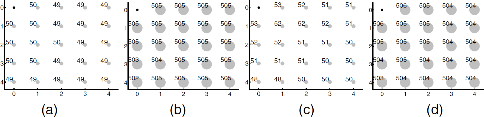
Dissemination progress for data of 1000 capsules with Go-back-N when (a) 5%, and (b) 50% of the time elapsed, and with selective retransmission when (c) 5%, and (d) 50% of the time elapsed. The radius of the circle at each sensor in the figure is proportional to the number of capsules received by the corresponding sensor.
The dissemination progress shown in Fig. 6(a-b) contradicts the dynamic behavior presented in Deluge [7]. Specifically, in [7], it has been shown that the data capsules reach the edge sensors in the network first before reaching the middle of the network. This dynamic behavior causes congestion (due to CSMA based MAC) in the middle and, hence, message communication and latency are increased. However, with Infuse (cf. Fig. 6(a-b)), we observe that all the sensors receive the data capsules at approximately the same time. And, Fig. 6(c-d) shows the dissemination progress with selective retransmission algorithm. Again, this result shows that the dissemination latency along the edges is similar to the latency along the diagonal.
In this section, we show that due to pipelining, dissemination latency remains almost the same for different network sizes, active radio time is significantly less than dissemination latency (and, hence, Infuse is
energy-efficient), and latency and active radio time grow linearly with respect to the data size.
Go-back-N algorithm. Figure 7 shows the results for dissemination with 1000 capsules for Go-back-N algorithm. With window size = 6, the latency is close to the analytical estimate (cf. Fig. 7(a)). If a sensor (say, j) missed a capsule, its predecessor (say, k) will retransmit the capsule. Since j could still get the same capsule from its other predecessors or its successors, unnecessary retransmissions are reduced with window size = 6. Furthermore, the latency and the active radio time remains almost the same for different network sizes. This result is also expected based on the pipelining property of the proposed protocol (cf. Section 4.1) and the analytical estimate, as ctot ≫ d. Additionally, when the window size increases, the sensors have to transmit more message during recovery, although most of the retransmissions may not be necessary. As a result, the recovery is too slow and, hence the latency increases. The same result can also be observed for message transmissions and receptions.
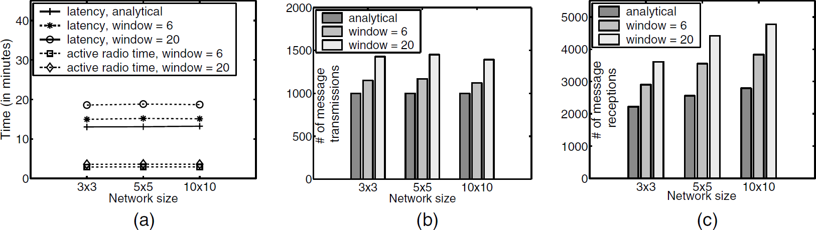
Simulation results for disseminating data with 1000 capsules using Go-back-N algorithm. (a) dissemination latency and active radio time, (b) number of message transmissions, and (c) number of message receptions.
Selective retransmission algorithm. Figure 8 shows the results for selective retransmission algorithm. Once again, the latency is close to the analytical estimate and remains almost the same for different network sizes (due to pipelining). If a sensor misses a capsule, its predecessors selectively retransmit the capsule, thereby reducing the number of retransmissions. Thus, the latency and the active radio time are reduced. Likewise, message transmissions/receptions are reduced.

Simulation results for disseminating data with 1000 capsules using selective retransmission algorithm. (a) dissemination latency and active radio time, (b) number of message transmissions, and (c) number of message receptions.
Latency and active radio time growth functions. Figure 9 shows how latency and active radio time grow with respect to the data size for both Go-Back-N and selective retransmission algorithms. As we can observe from the figure, both latency and active radio time grow linearly with respect to the data size.

Latency and active radio time growth functions for (a) Go-back-N based recovery algorithm and (b) selective retransmission based recovery algorithm.
Figure 10 shows the results for dissemination with 1000 capsules. The window size used in these simulations is 6. As expected, selective retransmission (SR) and selective retransmission algorithm with preferred predecessors (SR-PP) perform better than Go-back-N algorithm (GBN) and Go-back-N algorithm with preferred predecessors (GBN-PP) respectively (cf. Fig. 10(a)). This is due to the fact SR and SR-PP selectively retransmits lost capsules unlike GBN and GBN-PP. Moreover, the latency for SR-PP (respectively, GBN-PP) is more than SR (respectively, GBN).

Simulation results with preferred predecessors with 1000 capsules, (a) dissemination latency and (b) active radio time. Note that the scale is different for the two graphs.
For most situations, SR-PP (respectively, GBN-PP) has lower active radio time than SR (respectively, GBN). Thus, as expected, the use of preferred predecessor enables us to reduce the active radio time at the cost of increased latency. However, for large networks, the advantage of GBN-PP is no longer available; this occurs due to excessive retransmissions, as a sensor receives capsules from only one of its neighbors. By contrast, for GBN, the need for retransmissions is less, as a sensor receives redundant copies of a capsule. This effect is not seen while comparing SR and SR-PP, as unlike GBN and GBN-PP, a predecessor only retransmits the missing capsules and not the whole window. Hence, the effect of lost capsules in GBN-PP is more severe than that of SR-PP. With SR-PP, as the network size grows, active radio time reaches closer to that of SR, as the number of retransmissions in SR-PP is close to that of SR. (This is due to the fact the number of retransmissions by the preferred predecessors alone becomes closer to the number of retransmissions by all the predecessors of a sensor in SR.) Based on this result, we prefer SR and SR-PP compared to GBN and GBN-PP respectively. However, GBN and GBN-PP are easy to implement and GBN does not add any overhead to a message.
In these simulations, data consisting of 100 capsules are propagated across a 5 × 5 network. Fig. 11(a) shows the dissemination latency and active radio time for Go-back-N algorithm. With window size = 2, whenever a sensor (say, k) observes that its successor (say, j) misses a capsule, it initiates recovery by retransmitting the corresponding capsule. However, j can still receive the capsule from its other neighbors, as j has multiple paths to the base station. Hence, in this case, the recovery is initiated too early. Therefore, the latency is higher for window size = 2. For other values, predecessors allow the successors to recover from lost capsules through other neighbors. However, from Fig. 11(a), we observe that as the window size increases, the latency also increases. This is due to the fact if j misses a capsule, its predecessor k starts retransmitting the whole window from the lost capsule, although most of the retransmissions are not necessary. Thus, with Go-back-N, we observe that the window size should be chosen such that recovery is neither initiated too early nor too late. In Fig. 11(a), we note that with window size = 4, 6, …, 12, the latency remains almost the same.

Effect of window size. (a) Go-back-N and (b) selective retransmission algorithms.
Figure 11(b) shows the effect of window size on selective retransmission algorithm. In this figure, we observe that the dissemination latency (and active radio time) remains constant for window sizes ≥ 6. This is due to the fact that the predecessors selectively retransmit lost capsules, unlike Go-back-N algorithm. We note that the dissemination latency for window size = 2, 4 is slightly higher than that of other values. As discussed earlier in Go-back-N, in this case, if a sensor (say, j) misses a capsule, its predecessor (say, k) retransmits the corresponding capsule immediately, although j may receive the same capsule through other neighbors.
In these simulations, data consisting of 1000 capsules are propagated across the network. The window size used in these simulations is 6. The number of failed sensors in these simulations is 3 and 5 on a 5 × 5 network, and 3,5,10,20, and 27 on a 10 × 10 network. Figure 12 shows the effect of failed sensors on Go-back-N (GBN) and selective retransmission (SR) algorithms. From Fig. 12, the additional time required for dissemination in presence of failed sensors is small. When the number of failed sensors increases, this additional time also increases. This is due to the fact that the pipeline is disrupted when the sensors fail.

Effect of failed sensors. (a) Go-back-N and (b) selective retransmission. ∗ indicates bulk failure of 3 sub-grids of size 3 × 3.
With GBN, whenever a sensor observes that its successors miss a capsule, it retransmits the entire window. In other words, an inherent redundancy is available in GBN, where the sensor recovers all the successors (and possibly some predecessors) that have missed a capsule in the current window. However, with SR, in order to reduce the number of retransmissions, whenever a sensor observes that one of its successors has missed a capsule, it retransmits only the corresponding capsule. In other words, the level of redundancy is less in SR. Now, in the presence of failed sensors, the number of paths to base station is reduced. Due to the built in redundancy in GBN, the effect of the reduction in paths in GBN is less severe than that in SR (cf. Fig. 12).
Additionally, we did a simulation, where 3 sub-grids of size 3 × 3 are randomly selected as the failed sensors on a 10 × 10 network. From Figure 12, only 1.35 (respectively, 2.38) additional minutes are required to disseminate the data with GBN (respectively, SR). This value is close to the latency for dissemination in presence of 3 failed sensors. In other words, the cumulative effect of failure of nearby sensors shows up as a single disturbance in the pipeline. Therefore, the additional time required is less than the case where the failures are random.
Remark. In these simulations, we assumed that the sensors fail before the dissemination starts. Even if sensors fail during dissemination, the latency increases only by a very small percentage. Specifically, the latency is less than or equal to the latency in the case where the sensors have failed up front + the time required to detect the failure of sensors independently. Based on our simulations, the time required to detect failures is approximately 0.3 minutes. Thus, the latency in presence of dynamic failures increases only by a small percentage.
The goal of this section is to illustrate that Infuse could be used with different TDMA algorithms and with different topologies. In principle, it could be shown by changing one parameter at a time. We have performed simulations where we change one parameter (TDMA algorithm used with Infuse or the network topology) at a time and found that the results are consistent with the scenario where we change both the parameters. However, for brevity, we present the results where we used a different TDMA algorithm on a random deployment of 100 sensors.
We compare the performance of Infuse on a uniform deployment of 100 sensors in a 10 × 10 grid with a random deployment. For the uniform deployment, we use SS-TDMA [10], whereas we use the algorithm in [11] for random topology. (We note that the number of colors used to obtain TDMA schedule in both are approximately the same: 26 for grid topology and 31 for random topology.) The window size used in both simulations is 6. Table 2 summarizes the results of our simulations.
Infuse on a random topology using the TDMA algorithm from [11]

Infuse on a random topology using the TDMA algorithm from [11]
With Go-back-N algorithm (GBN), the latency required to disseminate 50 capsules on a random topology is 0.85 minutes and the active radio time is 0.14 minutes. In case of grid topology, the latency required is 0.78 minutes and the active radio time is 0.15 minutes. For disseminating data with 100 capsules, the latency required in grid topology is lesser than that of random topology. The active radio time in case of random topology is closer to that of grid topology and is less than that of selective retransmission (SR) algorithm.
With SR, for random topology, the latency required is higher than that of GBN. In case of GBN, during recovery, a sensor retransmits all the capsules in the window. Hence, it helps the successors that have missed a particular capsule in the current window to recover. By contrast, in case of SR, when a sensor detects that one of its successors lags behind, it retransmits the particular capsule. This helps only that successor to recover, unlike GBN, and, hence, the sensor has to learn the status of other successors in future slots. Thus, with random topologies, GBN performs better. We did not experience this behavior in case of grid topology as a sensor has at most two successors and, hence, retransmitting the whole window is expensive. Therefore, SR performs better on a grid topology and the active radio time is significantly less compared to random topology.
In this section, we summarize our results. First, in Section 4.1, we show that both Go-back-N and selective retransmission algorithms provide a uniform, fine-grained pipelining service. This ensures that Infuse does not have the dynamic behavior expressed in [7]. Also, in Section 4.2, we observe that the latency and the active radio time grow linearly with respect to data size for both the algorithms. Second, in Section 4.3, to our surprise, we observe that the use of preferred predecessors does not significantly improve the performance of Go-back-N algorithm. This is due to the fact that with preferred predecessors, duplicate sources are reduced. As a result, the probability of successfully retransmitting the entire window during recovery is reduced. By contrast, we do not observe this behavior with selective retransmission algorithm, as a sensor selectively retransmits only lost capsules during recovery. Third, in Section 4.4, we observe that the window size should be chosen carefully in case of Go-back-N. On the contrary, window size (≥ 6) does not affect the performance of selective retransmission algorithm. While selective retransmission performs better on a grid topology with no failures, from Sections 4.5 and 4.6, we observe that Go-back-N performs better in presence of failed sensors and on random topologies. Table 3 summarizes the results.
Comparison of recovery algorithms

Comparison of recovery algorithms
In general, in traditional networking, it is expected that selective retransmission be better than Go-back-N. From Table 3, we observe that for a grid topology with no failures, this is valid. However, if the network has a random topology or can be affected by failures, Go-back-N is better than selective retransmission. This is due to the fact that unlike SR, inherent redundancy is available in GBN, where a sensor recovers all the successors that have missed a capsule in the current window during recovery. Thus, this shows a somewhat counter-intuitive result that if the deployment may not be uniform or where sensors may fail, Go-back-N is preferable to selective retransmission.
Related work on dissemination has been addressed for wired networks in [24] where reliable transmission of multicast messages using multiple multicast channels is proposed. One of the important concerns in dissemination for wireless networks is the broadcast storm problem [25]. Specifically, in dissemination using naive flooding based algorithms, a broadcast storm is created where redundant broadcasts, contention, and collisions occur. Infuse is not affected by the broadcast storm problem since contention/collisions are managed by TDMA.
Network programming
Related work on dissemination protocols, especially for network programming in sensor networks, include Deluge [7] and multihop network reprogramming (MNP) [9]. Deluge is an epidemic protocol for disseminating large data objects that uses Trickle [26] to suppress redundant advertisements and requests, and to minimize the set of concurrent senders. MNP is a network reprogramming service that uses a sender selection algorithm to reduce the number of concurrent senders. Additionally, in MNP, sensors are allowed to turn their radio off whenever they are not transmitting or receiving new packets.
Comparison of Deluge and MNP with Infuse. In Table 4, we compare the simulation results of Deluge and MNP protocols with that of Infuse. Specifically, we compare the latency and the active radio time during dissemination of data of size 5.4 KB on a 10 × 10 network, where the interference ratio = 4. (We have chosen the data size as 5.4 KB based on the availability of results from [7,9].) The latency with Go-back-N (GBN) and selective retransmission (SR) algorithms is less than that of Deluge and MNP. Furthermore, the active radio time with Infuse (= 1.0 minutes for GBN) is significantly less than that of Deluge (= 11.67 minutes) and MNP (= 5.87 minutes). This is due to the fact that Infuse allows each sensor to turn its radio off in the slots not assigned to itself and its neighbors. In particular, for the grid topology, a sensor keeps its radio on only in the slots assigned to itself and to its 4 grid neighbors. Therefore, Infuse offers an energy-efficient dissemination service.
Go-back-N (GBN) and selective retransmission (SR) Vs. Deluge and MNP for dissemination on a 10
× 10 grid, where interference ratio = 4

Go-back-N (GBN) and selective retransmission (SR) Vs. Deluge and MNP for dissemination on a 10 × 10 grid, where interference ratio = 4
If the network density increases or the radio hardware is different then the interference ratio increases. Since Deluge and MNP use a CSMA based communication service, due to hidden terminal effect and network congestion, we expect that the latency and the active radio time would increase in such cases. In Infuse the TDMA period increases with interference ratio. As a result, the latency increases. However, the active radio time remains the same (cf. Table 5), as the sensor keeps its radio on only for 5 slots in each TDMA period.
Results for Go-back-N (GBN) and selective retransmission (SR) for dissemination of data of size 5.4 KB (=345 capsules) on a 10×10 network with different interference ratios (extrapolated from the results for interference ratio = 4)

Based on this comparison, we expect that Infuse will be highly beneficial in scenarios where the network is sparse and already deployed. However, in laboratory environments and in dense networks, the TDMA period may be very high. Hence, Infuse is not intended for such scenarios.
Other dissemination protocols
Other dissemination protocols include sensor protocols for information via negotiation (SPIN) [5], multihop over the air programming (MOAP) [6], and transport protocols [17, 28]. In SPIN, a 3-way handshake protocol (ADV/REQ/Data) is used to disseminate the data. Furthermore, meta-data (i.e. high-level descriptors of data) is used to declare the availability of new data. Infuse differs from SPIN in that no negotiations using meta-data are necessary and reliability is achieved through implicit acknowledgments. In MOAP, a publish-subscribe interface similar to [4] is used to provide dissemination (especially, reprogramming) service. In this scheme, a sensor has to receive the entire code before it can send meta-data about the availability of new code. MOAP uses sliding window mechanisms and negative acknowledgments for loss recovery. By contrast, with Infuse, each capsule is forwarded as soon as possible. And, Infuse uses sliding window mechanisms with implicit acknowledgments for loss recovery.
Work related to transport protocols in sensor networks is also used for data dissemination. Examples of transport protocols for sensor networks include pump slowly, fetch quickly (PSFQ) [28] and reliable multi-segment transport (RMST) [27]. These protocols rely on negative acknowledgments for loss recovery. By contrast, Infuse uses implicit acknowledgments in order to recover lost capsules. Additionally, Infuse takes advantage of the underlying TDMA based MAC in providing a pipelined service.
We implemented Infuse on TinyOS for Mica-2 and XSM motes. In the DARPA NEST meeting on extreme scaling in sensor networks (ExScal demonstration, Avon Park, FL, December 2004) [1], we demonstrated Infuse on Mica-2 motes to reprogram the network with a new program, using Go-back-N based recovery algorithm.
We demonstrated Infuse on a 5×5 grid with inter-sensor separation of 8 ft. We integrated Infuse with SS-TDMA [10] to assign time slots to each sensor. We used a conservative estimate of interference ratio, y=6. Initially, the base station contained the new data (i.e., new program for the sensors) The size of the new program was 2 KB (=128 capsules). First, the base station established the TDMA schedule according to the SS-TDMA algorithm. Then, it disseminated the program capsules, one in each of its TDMA slots. In this experiment, the disseminated the program capsules, one in each of its TDMA slots. In this experiment, the dissemination latency was 3.5 minutes. The active radio time during the dissemination process was approximately 25 seconds. These results are close to the analytical estimate for latency (= 3.37 minutes) and active radio time (= 19.2 seconds).
We found similar results in other experiments at Michigan State University. We have experimented with Infuse for reprogramming the network with programs of size from 2 KB–15 KB, interference ratio of 4–6 and window size of 6–12. In all these experiments, the results were consistent with the analytical estimate/simulation results.
Discussion
In this section, we discuss some of the questions raised by this work.
How does Infuse perform for different interference ranges or network densities?
In [21,22], it has been shown that a signal from a (Mica based) sensor (say, j) reaches a sensor within distance 10 m (called, connected region or communication range) with probability ≥ 98%. And, the sensors at distance 10–32 m (called, transitional region or interference range) receive the signal from j with a reduced probability. Finally, the sensors at distance > 32 m (called, disconnected region), do not receive the signal from the sender. Based on this discussion, the ratio of the interference range to communication range is around 3.2. If the network density increases (or a different sensor/radio hardware is used) then this ratio may increase. As a result, more sensors may fall in the transitional region. Therefore, the interference ratio would have to be increased. Figure 13 shows the performance of Infuse with different interference ratios. As the ratio increases, the latency also increases. For a given interference ratio, the latency grows linearly with respect to the data size. Moreover, in case of grid topology, the number of slots for which a sensor keeps its radio on is approximately 5 × the number of capsules (one slot to forward, 4 slots to listen to its grid neighbors). Hence, the active radio time is independent of the interference ratio.

Effect of interference ratio on dissemination latency.
In case of even larger values of interference ratio, the probability that a given message reaches a longer distance increases. Towards this end, we can use the SS-TDMA algorithm customized for larger communication ranges [10]. In this approach, not all sensors are required to forward the data. Specifically, the sensors that are farther away from the sender can forward the data. In case of random topologies, we can organize the network into clusters and clect cluster heads/leaders [12]. Alternatively, we can compute the minimum connected dominating set or MCDS (similar to Sprinkler [29]). Once the leaders or the sensors in MCDS are identified, we can establish a TDMA schedule (e.g., using [11,12]) for them. The remaining sensors can then listen to the slots assigned to their closest leaders or sensors in MCDS. Thus, Infuse can be easily modified to disseminate data in high density networks.
What is the tradeoff in using preferred predecessors?
In Section 2.2, we proposed a heuristic that allows the sensors to reduce the number of message receptions during the dissemination process. This heuristic allows each sensor to select one of its predecessors as its preferred predecessor. The sensor now listens to slots assigned to its preferred predecessor. This preferred predecessor is responsible for recovery from lost capsules at the sensor. Other predecessors can turn their radio off in the slots assigned to this sensor. Thus, the number of duplicate receptions are reduced. As a result, energy usage and number of message receptions during dissemination are reduced.
With this mechanism, the effective diameter of the network may be increased, since a sensor listens only to its preferred predecessor. However, as shown in Section 3, once the first capsule is propagated across the network, the rest of the capsules can be propagated in a pipeline fashion. As observed in Fig. 10(a), the dissemination latency for data containing 1000 capsules remains almost the same in 3×3, 5×5, and 10×10 networks. Hence, even if the diameter of the network increase, the dissemination latency does not increase significantly (cf. Section 4.3 for simulation results). However, in case of Go-back-N based recovery algorithm, the active radio time increases for larger networks as the sensors have to rely on their preferred predecessors for loss recovery, thereby, increasing the number of retransmissions. By contrast, the active radio time is reduced with selective retransmission based recovery algorithm. This is due to the fact that only the lost capsules are retransmitted by the preferred predecessors (unlike Go-back-N algorithm).
Can we use Infuse to disseminate data in large scale networks?
Yes. Towards this end, first, we note that the dissemination latency does not increase significantly as the network diameter increases (cf. Figure 10(a)). In applications such as [1,2], where 1000's of sensors are deployed in a large field, the network is typically partitioned into several sections. We can use Infuse to disseminate data in each section independently and simultaneously. Thus, the whole network can be updated with the new data in the time it takes to disseminate the data across a single section.
In this paper, we presented Infuse, a TDMA based data dissemination protocol for sensor networks. To deal with random message losses caused by varying link properties and message corruption, we considered two recovery algorithms based on the sliding window protocols that use implicit acknowledgments. The first algorithm, Go-back-N, adds no extra information to the payload of a message. With Go-back-N, we showed that the window size should be chosen carefully. And, we observed that Go-back-N tolerates failed sensors without significant degradation. The second algorithm, selective retransmission adds 2b extra bits to the message, where 2b is the size of the window. With selective retransmission, we showed that window size (≥ 6) does not affect the protocol. However, in the presence of failed sensors, we showed that it increases latency considerably. Thus, we find a somewhat counter-intuitive result that Go-back-N is preferable to selective retransmission if the topology is not uniform or if failures may occur.
In the presence of no channel errors, we estimated the dissemination latency. We showed that the data is propagated in a pipeline and, hence, the latency is reduced. We argued that Infuse is energy-efficient. Specifically, we showed that message transmissions/receptions are reduced. Since Infuse uses a TDMA based MAC protocol, sensors need to listen to the radio only in the slots assigned to their neighbors. In the remaining slots, sensors can turn off their radio. Moreover, we proposed an algorithm to reduce messages receptions and the active radio time further by using the notion of preferred predecessors.
Reliable data dissemination is a bandwidth intensive and time consuming operation. Hence, it has the potential to disrupt the communication of the underlying application. In a CSMA based network, this disruption is expected to be severe, as the network is highly congested. By contrast, a TDMA based protocol can provide some guarantees about the communication of the underlying application. Since the application messages (e.g., event messages) are rare and are time critical, the TDMA algorithm can be extended to provide high priority for such messages. The TDMA algorithm can also be customized (e.g., using [10]) for the communication pattern of the application. Thus, the TDMA algorithm can communicate such rare messages reliably. In this context, in [10], we have compared the performance of CSMA with SS-TDMA. Specifically, if the only communication consists of event messages, SS-TDMA improves the reliability from 50% to 100% with a small increase in the delay. It follows that if event messages have to compete with bandwidth intensive dissemination then a TDMA based service such as Infuse will be especially useful.
We have implemented Infuse in TinyOS [15] for Mica based sensor devices. We applied Infuse to reprogram a 5×5 network with a program of size from 2 KB-15 KB. The latency, active radio time, message transmissions/receptions are close to the simulation results discussed in this paper. We have demonstrated Infuse to the DARPA NEST team during the ExScal project demonstration in Avon Park, FL, December 2004 [1].