Maximizing Data Extraction in Energy-Limited Sensor Networks

Abstract

We examine the problem of maximizing data collection from an energy-limited store-and-extract wireless sensor network, which is analogous to the maximum lifetime problem of interest in continuous data-gathering sensor networks. One significant difference is that this problem requires attention to “data-awareness” in addition to “energy-awareness”. We formulate the maximum data extraction problem as a linear program and present a 1 + ω iterative approximation algorithm for it. As a practical distributed implementation we develop a faster greedy heuristic for this problem that uses an exponential metric based on the approximation algorithm. We then show through simulation results that the greedy heuristic incorporating this exponential metric performs near-optimally (within 1 to 10% of optimal, with low overhead) and significantly better than other energy aware routing approaches (developed mainly through intuition), particularly when nodes are heterogeneous in their energy and data availability.

Keywords

Sensor Networks Mathematical Programming/Optimization Network Flows

I. Introduction

In many sensor network applications involving environmental monitoring in remote locations, planetary exploration and military surveillance, it is neither necessary nor even possible for a user to obtain data from the network continuously, in real time. In such applications, the information from the entire network can be extracted en masse after a prolonged period of sensing and local storage. This process of extraction can be done by a stationary sink or a mobile sink (robot). However, since communication is often the most expensive operation for a sensor node, the limited batteries may make it impossible to collect all the data stored in the network. We examine the problem of maximizing the data extracted (by a stationary sink) from such an energy-limited sensor network consisting of heterogeneous nodes. The maximum data extraction problem is an analog of the maximum lifetime problem of interest in continuous data-gathering sensor networks [1], [2], [3], [4] that has been studied previously. However, this problem introduces an additional element of “data-awareness” that must be considered in addition to “energy-awareness”.

We first show how the maximum data extraction problem can be formulated as a linear program. We then adapt and extend techniques for multi-commodity flow problems first developed by Garg and Koenemann [5] to develop an iterative algorithm for our problem with a provable (1 + ω) approximation. This algorithm suggests a new link metric (involving the remaining energies of both sender and receiver nodes, the distance between them, and the data level at the sender) that we then used to develop a fast, practically implementable, distributed heuristic that we refer to E-MAX. The heuristic uses a selfish strategy in that each sensor gives priority to transmitting its data before relaying that of other nodes. Our simulations show that this sophisticated heuristic (obtained from the analysis) offers near-optimal performance under all conditions, and significantly better compared to other energy aware solutions (mainly developed by intuition) particularly when nodes are heterogeneous in their energy and data availability.

The rest of the paper is organized as follows. In section II, we discuss related work to place our contributions in context. We define the problem and present the LP formulation and its dual in section III. An interpretation of the LP dual suggests the 1 + ω iterative approximation algorithm that we present and analyze in section IV. We discuss the implementation of this algorithm in section V. We present fast implementable heuristics in section VI. Simulation results comparing these implementations are presented in section VII. Concluding comments are provided in section VIII.

II. Related Work

Our work is inspired by a vast body of literature related to optimizing the performance of ad hoc and sensor networks. We outline a few of these studies that are very close in spirit to our work.

A. Energy Aware Routing

Most of the literature in this area has focused on routing techniques that extend the life time of a sensor or ad hoc network by taking into account remaining battery energy. In [6], Toh has proposed the Conditional Max-Min Battery Capacity Routing (CMMBCR), which selects the shortest path for routing data from one node to the other in an ad hoc network such that all nodes on the path have remaining battery power above a certain threshold. Singh et al. [7] present an elaborate study of 5 different metrics which are all a function of the node battery power and conclude that these metrics can give significant energy savings over naive hop-count-based metrics. In [8], Kar et al. propose an online algorithm for routing messages in an ad hoc network, also based on the remaining battery energy of a node.

Energy efficient routing techniques have also been proposed in several studies on sensor networks. Heinzelman et al. propose a family of adaptive protocols called SPIN for energy efficient dissemination of information throughout the sensor network [9]. In [10], Heinzelman et al. propose LEACH, a scalable adaptive clustering protocol in which nodes are organized into clusters and system lifetime is extended by randomly choosing the cluster-heads. Lindsey et al. propose an alternative data gathering scheme called PEGASIS in [11], in which nodes organize themselves in chains, also with rotating elections, for communicating data. Lindsey et al [12] study data gathering schemes that explore the trade-off between energy consumed and delay incurred.

The problem of maximum data extraction introduces “data-awareness” as an important factor for routing data in addition to “energy-awareness” as we discuss in section II-B. This problem can also be formulated as a multi-commodity flow problem. There is a vast literature on algorithms for multi-commodity flow problems and their application to networking. Hence we next discuss studies in this area which are relevant to our work.

B. Multi-Commodity Flow Algorithms

The multi-commodity flow problem is of great practical importance and theoretical interest. The problem deals with finding a routing scheme to maximize the total quantity of several different commodities (each possibly having different sources and sinks) sent over a network with restricted capacity.

Maximizing the lifetime of a sensor (or ad hoc) network can be formulated as a multi-commodity flow problem. In [13] Chang et al. also use the multi-commodity flow formulation for maximizing the lifetime of an ad hoc network. They propose a class of flow augmentation and flow redirection algorithms that balance the energy consumption rates across nodes based on the remaining battery power of these nodes. This approach seems to considerably increase the network lifetime. Brown et al. propose a novel power aware routing objective i.e. the maximum flow life curve that maximizes traffic flow utility over time [14]. They propose an LP-based algorithm for maximizing this objective. Bhardwaj and Chandrakasan [3] examine feasible role assignments (FRA) of nodes as a means of maximizing the lifetime of aggregating as well as non-aggregating sensor networks, and also make use of linear programs based on network flows. Kalpakis et al. examine the MLDA (Maximum Lifetime Data Aggregation) problem and the MLDR (Maximum Lifetime Data Routing) problem in [2], again formulating it as an LP using multi-commodity network flows. They observe that as the network size increases, solving the LP takes considerable time and propose some clustering heuristics to achieve near-optimal performance.

As the size of the LP increases, it becomes desirable to solve this problem approximately but quickly. Garg et al. present an excellent discussion of the current fast approximation techniques for solving the multi-commodity flow problem [5]. They propose a simple polynomial time iterative algorithm that gives a (1 + ∊) approximation to the multi-commodity flow problem and some other fractional packing problems. The algorithm associates a length with each edge. In each iteration, the algorithm routes flow over the shortest path. After routing the flow, the algorithm increases the length of all the edges along the shortest path. This is done so that subsequent flow may be routed over an underutilized path. This process continues till the shortest path (using the length metric) exceeds 1. However, at this point, it is possible that some links might be over-utilized (i.e. in excess of their capacity). The algorithm then scales down all the flows by a factor of the maximum over-utilization. This is a beautiful algorithm that explains the nature of the routing scheme needed to maximize the flow in a multi-commodity flow problem. The algorithm as stated needs some modifications for it to be applied to an ad hoc network context. While Chang et al. in [1] have also previously applied the Garg-Koenemann algorithm to ad-hoc network lifetime maximization, there are significant difference between [1] and our work that we describe below.

In this paper, we modify and extend the application of the Garg-Koenemann algorithm to the problem of maximizing data collection in store-and-extract sensor networks. Receptions are assumed to consume battery power, unlike [1] [4]. Also, the above studies in the multi-commodity flow problem do not restrict the amount of flow of each commodity [1] [2] [4] [5] [13]. With unrestricted flows, the solution for the maximum data extraction problem would be trivial in that nodes near the sink would monopolize the entire flow. We are interested in the case where sensors generate a finite amount of data i.e. the flow of each commodity is finite. Thus as mentioned at the end of section II-A, the maximum data-extraction problem introduces the data availability at each node as an important routing concern, in addition to the “energy-awareness” previously discussed in the literature. A similar problem was quite recently studied by Hong et al. in the context of sensor networks that use short range communication [16]. They assume that while transmissions and receptions over all links cost the same, the capacity of a link decreases with distance. This formulation helps them to develop a completely decentralized algorithm which is a variant of the Push-Relabel algorithm [17]. However their algorithm may be unsuitable for the model used in this study where transmissions costs are a function of distance between the sender and the receiver.

In this paper, besides developing an LP formulation for the maximum data-extraction problem (using a radio model that includes both transmission and reception costs) and extending the application and analysis of the Garg-Koenemann approximation algorithm for it, we also present a practical distributed heuristic based on this algorithm that is shown to outperform other energy aware routing approaches, particularly in heterogeneous conditions where nodes have varying data and energy availability.

III. Problem Definition

Consider a scenario where several sensors that are deployed in a remote region have completed their sensing task and have some locally stored data. We are interested in collecting the maximum amount of data possible from all these sensors at a sink node T, given some remaining energy constraints in each of these sensors.

Figure 1 shows a sample scenario. Each node i is labelled with its (x,y) coordinates, its available data and remaining energy. The goal is to extract all this data to the sink node. The arrows and the indicated flows on each indicate the optimal solution for this particular example obtained by using the LP we describe in the next section.

Figure 1

Illustration of a sample scenario with optimal solution to the maximum data extraction problem. Solution assumes β_t = 32.4μJ/byte/km² and β_r = 400nJ/byte

We now present the formal model for the problem.

A. Model

Let N be the total number of sensors. Let T be the target (sink) to which the data is to be sent. Let $D_{m a x}^{j}$ be the amount of data (bytes) collected by sensor j, where $D_{m a x}^{j} > 0. e_{m a x}^{j}$ is the residual energy of sensor j. These sensors are arbitrarily deployed in a region. d_ij is the Euclidean distance between sensors i and j. A sensor i can communicate with any sensor j which is within the communication range R from it. Thus, this communicating range overlays a connectivity graph G = (V, E), where |V| = N. An edge (i, j) ∊ E if d_ij ≤ R.

The energy consumed in transmitting a unit byte from one sensor to the other depends on the distance between them. Tx_ij is the energy consumed in transmitting a single byte from sensor i to j. Tx_ij is assumed to be proportional to the $d_{i j}^{2} (i, e . {Tx}_{i j} = β_{i} d_{i j}^{2})$ , where β_t > 0. R_ij is the energy consumed at sensor j for receiving a single byte of data from sensor i. R_ij is assumed to be independent of the distance d_ij. Let R_ij = β_r where β_r > 0.

For the ease of modelling, we add a fictitious source S, such that there exists an edge from S to every other node in V, except T. Also, add an edge from T to S. Let this new graph be G′. Thus, G′ = (V′, E′), where V′ = V ∪ S and E′ = E ∪ {(S,i)} ∪ {(T,S)}, where i ∊ V, i ≠ T. As will be shown later in section III-B, the location of the fictitious source S can be arbitrary.

The problem of collecting the maximum possible data from these energy constrained sensor nodes can be formulated as multi-commodity flow problem. As shown later in sections III-B and III-C, the addition of S and its associated links simplifies the LP formulation for the multi-commodity flow problem and our analysis.

B. Linear Program (LP) Formulation

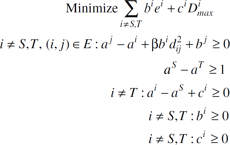
In this section, we formulate the maximum data collection problem as an LP. The constraints of the LP are

Flow Conservation: The amount of data transmitted by a node is equal to sum of the amount of data received by the node and the amount of data generated by the node itself.

Energy Constraint: The amount of data received and transmitted by a node is limited by the energy of the node. However, there are no energy constraints for the fictitious source S and the sink T.

Let f_i,j be the amount of data transmitted form node i to node j. The LP can now be formulated as follows:

\begin{aligned} Maximize f_{T, S} such that \\ \sum_{j = 1}^{N} f_{j, i} - \sum_{j = 1}^{N} f_{i, j} = 0 \\ i \neq S, T : β \sum_{(i, j) \in E} f_{i, j} d_{i, j}^{2} + \sum_{(j, i) \in E} f_{j, i} \leq e^{i} \\ i \neq S, T : f_{S, i} \leq D_{m a x}^{i} \\ (i, j) \in E^{'} : f_{i, j} \geq 0 \end{aligned}

(1)

where

β = \frac{β_{t}}{β_{r}}

(2)

i \neq S, T : e_{i} = \frac{e_{m a x}^{i}}{β_{r}}

(3)

Note that we have normalized the energy in terms of receptions i.e. each reception costs a unit of energy, while each transmission from (i, j) costs $β d_{i j}^{2}$ units, where β ≥ 1.

By adding the fictitious source S and its associated links, we have made the following transformations to the multi-commodity flow problem:

The amount of data transmitted by S to any node i is equal to the amount of data $D_{m a x}^{i}$ generated at node i. The reception of this data from S does not incur any energy consumption. Hence, as we mentioned in section III-A, the placement of S does not affect the solution.

Note that since the flow conservation is satisfied by both the fictitious source S and the target T, all the data received by the target will be transmitted to the source S, which in turn will be equal to the amount of data transmitted by the source S.

The problem now becomes one of maximizing the circulation of the commodities from S to T and back. The advantage of this will become apparent in section III-C.

The above LP can be solved to compute the maximum amount of data that can be collected from the N sensors. It would also give the amount of data (flow) that should be sent from sensor i to sensor j.

However, in this study we are interested in proposing a constructive algorithm that maximizes the amount of data collected. For this purpose, we attempt to understand the structure of the primal LP solution by examining the dual LP in section III-C.

C. Dual LP Formulation

The dual of the LP is as follows:

\begin{aligned} Minimize \sum_{i \neq S, T} b^{i} e^{i} + c^{i} D_{m a x}^{i} \\ i \neq S, T, (i, j) \in E : a^{j} - a^{i} + β b^{i} d_{i j}^{2} + b^{j} \geq 0 \\ a^{S} - a^{T} \geq 1 \\ i \neq T : a^{i} - a^{S} + c^{i} \geq 0 \\ i \neq S, T : b^{i} \geq 0 \\ i \neq S, T : c^{i} \geq 0 \end{aligned}

(4)

Let a, b, and c be vectors such that their i'th element is denoted by aⁱ, bⁱ and cⁱ respectively. Let

A (b, c) = \sum_{i \neq S, T} b^{i} e^{i} + c^{i} D_{m a x}^{i}

(5)

that is, A(b, c) is the objective function of the dual LP. The above dual has the following interesting interpretation:

Let l(b, c) be a length metric and let l_i,j (b, c) be the length of edge (i, j) in this metric.

Then, if

l_{i, j} (b, c) = {\begin{cases} β b^{i} d_{i j}^{2} + b^{j} & i f i \neq S \\ c^{i} & i f i = S, j \neq T \end{cases}

(6)

The dual LP can be re-written as follows:

\begin{aligned} Minimize A (b, c) such that \\ i \neq T, S : l_{i, j} (b, c) \geq a^{i} - a^{j} \\ a^{S} - a^{T} \geq 1 \\ l_{S, i} (b, c) \geq a^{S} - a^{i} \end{aligned}

(7)

Consider an arbitrary S-T path P. Let P be S, i₁, i₂, … i_k, T. Now, the length of path P can be written as follows:

\begin{aligned} l (P) & = l_{S, i} (b, c) + l_{i_{k}, T} (b, c) + \sum_{z = 1}^{k - 1} l_{i_{z}, i_{z + 1}} (b, c) \\ \geq (a_{S} - a_{i_{1}}) + (a_{i_{k}} - a_{T}) + a_{i_{1}} - a_{i_{k}} (from Eqn, 7) \\ \geq a_{S} - a_{T} \\ \geq 1 \end{aligned}

(8)

Thus, the length of any arbitrary S-T path in the l(b, c) metric is greater than or equal to 1, which implies that the length of the shortest path in the l(b, c) metric should also be greater than equal to 1. Thus, by transforming the primal LP in section III-B into a circulation problem, we get a very simple value (i.e., 1) for the length of the shortest path in the l(b, c) metric.

Let P(b, c) be the shortest path in the metric l(b, c) and α(b, c) be the length of this shortest path. Thus, the objective of the dual LP is to minimize A(b, c) such that α(b, c) ≥ 1. This is equivalent to minimizing $\frac{A (b, c)}{α (b, c)}$ .

Let

ς = M i n {\frac{A (b, c)}{α (b, c)}}

(9)

The above interpretation of the dual LP leads to a simple algorithm which approximates the optimal value of the primal. We specify the algorithm and analyze it in section IV.

IV. Approximation Algorithm

We propose an iterative algorithm which is a modification of the Garg-Koenemann algorithm [5]. Before proposing the algorithm, we introduce a few notations. Let

$b_{j}^{i}$ be the value of b_i in the j'th iteration. Initially, b₀ = c₀ = δ i.e., $\forall i : i \in V^{'} : b_{0}^{i} = c_{0}^{i} = δ$ . The choice of δ is discussed in section IV-B.

f_j be the total T-S (or S-T) flow till the j'th iteration. Initially, this flow is zero (i.e., f₀ = 0).

A(j) = A(b_j, c_j) be the value of the dual objective function after iteration j.

P_j = S, i₁, i₂, … i_k, T be the shortest S-T path in the l(b_j, c_j) metric (at iteration j)¹ On P_j, let i₀ = S and i_k+1 = T.

α(j) = α(b_j, c_j) be the length of the shortest S-T path after iteration j.

Moreover, ∀i ∊ V′, node i has a capacity associated with it. The capacity of a node depends on where it appears in an S-T path. Hence, we define the capacity of a node with respect to some path P = S, i₁, i₂, …i_k, T in which it appears. The capacity κ(i) of each node in this path is modelled as follows:

\begin{aligned} κ (S) & = D_{m a x}^{i_{1}} \\ κ (i_{1}) & = \frac{e_{m a x}^{i_{1}}}{β d_{i_{1}, i_{2}}^{2}} \\ κ (i_{2}) & = {\frac{e_{m a x}^{i_{z}}}{1 + β d_{i_{z}, i_{z + 1}}^{2}}} for 1 < z \leq k \end{aligned}

(10)

The algorithm is as follows:

j = 0

while (α (j) < 1) do

Select the shortest S-T path P_j.

Route c units of data along this path, where c is given as follows:

c = {Min}_{0 \leq z < k {κ (i_{z})}}

i.e., “saturate” the shortest path.

Update the vectors b and c as follows:

\begin{aligned} For 1 & < z \leq k, \\ b_{j}^{i_{z}} & = b_{j - 1}^{i_{z}} {1 + \frac{ε c β d_{i_{z}, i_{z + 1}}^{2}}{e^{i_{z}}}} + \frac{ε c}{e^{i_{z}}} \\ For z & = 1, \\ c_{j}^{i_{1}} & = c_{j - 1}^{i_{1}} {1 + \frac{ε c}{D_{m a x}^{i_{1}}}} \\ b_{j}^{i_{1}} & = b_{j - 1}^{i_{1}} {1 + \frac{ε c β d_{i_{1}, i_{2}}^{2}}{e^{i_{1}}}} \end{aligned}

f_j=f_j−1+c

j=j+1

On termination, f_j gives the value of the total data collected. While choosing the shortest S-T path, the algorithm accounts for the battery utilization (fraction of the battery power utilized) as well as the data utilization (fraction of the data sent) at each sensor. Thus, the algorithm, as mentioned earlier in section II is both “energy-aware” and “data-aware”.

We analyze the approximation ratio of the algorithm in section IV-A.

A. Analysis

Initially, the value of the objective function of the dual LP is given as

\begin{aligned} A (0) & = \sum_{i \neq S, T} b_{0}^{i} e^{i} + c_{0}^{i} D_{m a x}^{i} \\ = \sum_{i \neq S, T} δ e^{i} + δ D_{m a x}^{i} \end{aligned}

(11)

On a subsequent iteration j, the objective function is given as follows:

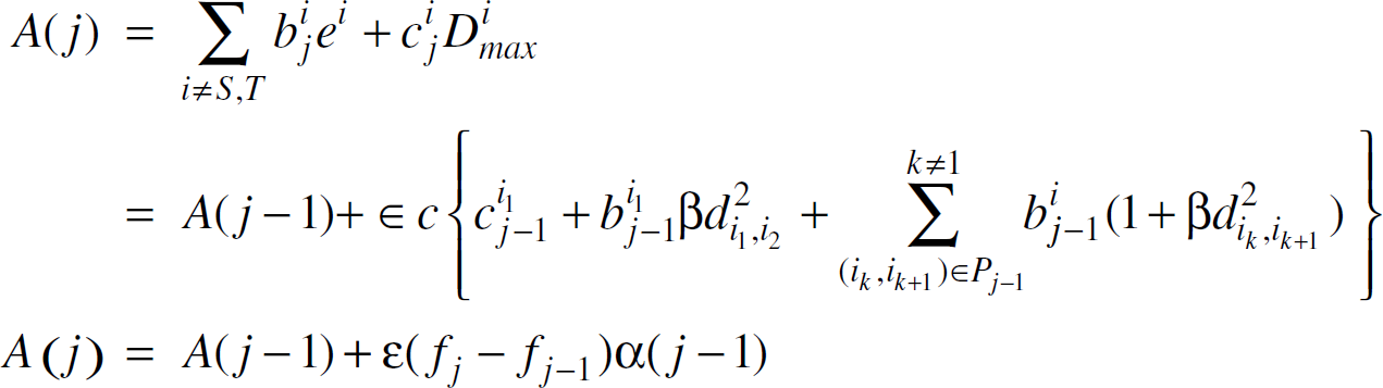
\begin{aligned} A (j) & = \sum_{i \neq S, T} b_{j}^{i} e^{i} + c_{j}^{i} D_{m a x}^{i} \\ = A (j - 1) + \in c {c_{j - 1}^{i_{1}} + b_{j - 1}^{i_{1}} β d_{i_{1}, i_{2}}^{2} + \sum_{(i_{k}, i_{k + 1}) \in P_{j - 1}}^{k \neq 1} b_{j - 1}^{i} (1 + β d_{i_{k}, i_{k + 1}^{2}})} \\ A (j) & = A (j - 1) + ε (f_{j} - f_{j - 1}) α (j - 1) \end{aligned}

(12)

Solving the above recurrence, we get

A (j) = A (0) + ε \sum_{l = 1}^{j} (f_{l} - f_{l - 1}) α (l - 1)

(13)

If each element of b_j and c_j is decreased by b₀ = c₀ = δ, then the objective function of the dual LP is given as follows:

\begin{aligned} A (b_{j} - δ, c_{j} - δ) & = \sum_{i \neq S, T} (b_{j}^{i} - δ) e^{i} + (c_{j}^{i} - δ) D_{m a x}^{i} \\ = \sum_{i \neq S, T} b_{j}^{i} e^{i} + c_{j}^{i} D_{m a x}^{i} - \sum_{i \neq S, T} δ e^{i} + δ D_{m a x}^{i} \\ A (b_{j} - δ, c_{j} - δ) & = A (j) - A (0) \end{aligned}

(14)

Let the shortest path P of length αj be S, i₁, i₂, … i_k, T. That is, α_j = l_P (b_j, c_j) Now, the length of P_j in the metric l(b_j – δ, c_j – δ) is given as follows:

\begin{aligned} l_{P_{j}} (b_{j} - δ, c_{j} - δ) = & l_{S, i_{1}} (b_{j} - δ, c_{j} - δ) + l_{i_{1}, i_{2}} (b_{j} - δ, c_{j} - δ) \\ + \sum_{(i_{k}, i_{k + 1}) \in P_{j}}^{k \neq 1} l_{i_{k}, i_{k + 1}} (b_{j} - δ, c_{j} - δ) \\ = & (c_{j}^{i_{1}} - δ) + (b_{j}^{i_{1}} - δ) β d_{i_{1}, i_{2}}^{2} + \sum_{(i_{k}, i_{k + 1}) \in P_{j}}^{k \neq 1} (b_{j}^{i_{k}} - δ) (β d_{i_{k}, i_{k + 1}}^{2} + 1) \\ = & α (j) - δ {1 + β d_{i_{1}, i_{2}}^{2} + \sum_{(i_{k}, i_{k + 1}) \in P_{j}}^{k \neq 1} (β d_{i_{k}, i_{k + 1}}^{2} + 1)} \end{aligned}

Thus,

α (b_{j} - δ, c_{j} - δ) \geq α (j) - δ L

(15)

where L is the largest value of

1 + β d_{i_{1}, i_{2}}^{2} + \sum_{(i_{k}, i_{k + 1}) \in P_{j}}^{k \neq 1} (β d_{i_{k}, i_{k + 1}}^{2} + 1)

Now, from Eqn. 9 in section III-C

\begin{aligned} ς & \leq \frac{A (b_{j} - δ, c_{j} - δ)}{α (b_{j} - δ, c_{j} - δ)} \\ \leq \frac{A (j) - A (0)}{α (j) - δ L} \\ α (j) & \leq δ L + \frac{\in}{ς} \sum_{i = 1}^{j} (f_{i} - f_{i - 1}) α (i - 1) \end{aligned}

(16)

Now, in order to get an upper bound on α(j), we let all the α(i)'s where 1 ≤ i ≤ j − 1 to be as large as possible, i.e., ∀i: 1 ≤ i ≤ j − 1,

α (i) = δ L + \frac{ε}{ς} \sum_{l = 1}^{i} (f_{l} - f_{l - 1}) α (l - 1)

(17)

Thus,

\begin{aligned} α (j) & \leq α (j - 1) + \frac{ε}{ς} (f_{j} - f_{j - 1}) α (j - 1) \\ \leq α (j - 1) (1 + \frac{ε}{ς} (f_{j} - f_{j - 1})) \\ \leq α (j - 1) e^{\frac{ε}{ς} (f_{0} - f_{j - 1})} \\ α (j) & \leq α (0) e^{\frac{ε}{ς} f_{j}} \\ α (j) & \leq δ L e^{\frac{ε}{ς} f_{j}} \end{aligned}

(18)

Thus, at iteration t, when the shortest S-T path has length greater than or equal to 1, the following inequality holds

\begin{aligned} 1 \leq α (t) \leq δ L e^{\frac{ε}{ς} f_{t}} \\ \frac{ς}{f_{t}} \leq \frac{ε}{l n (\frac{1}{δ L})} \end{aligned}

(19)

Thus, despite the modifications to the Garg-Koenemann algorithm to adapt it to our problem, we see that the bound obtained in the above inequality is exactly the same as that obtained in [5].

Although the algorithm chooses the shortest path based on data and energy utilization of nodes along the path, neither the remaining energy nor the remaining data at each sensor is actively monitored. Hence, it would be interesting to see if the flow f_t is feasible. We analyze the feasibility of the flow in section IV-B.

B. Scaling

Whenever bⁱ of a node i has increased, the node has been on a path whose length is strictly less than 1. If this had not been the case, the shortest S-T path had a length greater than 1 and the algorithm should have terminated. Moreover, the bⁱ is increased by a factor of at most (1 + ∊). Thus $b_{t}^{i} < (1 + ε)$ . Now, if bⁱ is increased x times during the execution of the algorithm, in the worst case all these x increase operations completely utilize the energy eⁱ of node i. Thus, in the worst case $b_{t}^{i} = δ (1 + ε)^{x} < 1 + ε$ , which implies that $x < l o g_{1 + ε} (\frac{1 + ε}{δ})$ . The factor by which the node i is over-utilized is i is x. Thus by scaling f_t down by a factor of $l o g_{1 + ε} (\frac{1 + ε}{δ})$ , we can ensure that the energy constraint is not violated.

If bⁱ is increased x times, cⁱ is also increased at most x times. Thus, it can be seen that even the data constraint is violated by at most a factor of $l o g_{1 + ε} (\frac{1 + ε}{δ})$ . Thus, a single scaling operation ensures that both the energy and the data constraints are satisfied.

Thus, there exists a feasible flow of value $\frac{f_{t}}{l o g_{1 + ε} (\frac{1 + ε}{δ})}$ .

Similar to [5], the ratio of the values of the dual to the primal solutions is

γ = \frac{ς}{f_{t}} l o g_{1 + ε} \frac{1 + ε}{δ}

As shown in [5], if

δ = (1 + ε) ((1 + ε) L)^{- \frac{1}{ε}}

(20)

γ \leq (1 - ε)^{- 2}

(21)

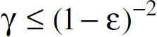
Thus to get within a factor of (1 + ω)of the optimal, ∊ is given as follows:

ε \leq \sqrt{\frac{1}{1 + ω}}

(22)

Thus, the algorithm mentioned in section IV can solve the multi-commodity flow problem and produce results arbitrarily close to optimum.

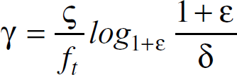
Number of Iterations

From the analysis in this section, we observe that the factor by which a node i's energy is over-utilized is at most $l o g_{1 + ε} \frac{1 + ε}{δ}$ . Thus, the number of iterations in which i is the bottleneck on the shortest path is at most $l o g_{1 + ε} \frac{1 + ε}{δ}$ . There are a total of N nodes, and thus, the total number of iterations is $O (N l o g_{1 + ε} \frac{1 + ε}{δ})$ .

In the next section, we discuss a few issues that might be important for the implementation of the approximation algorithm in a sensor network.

V. Implementation of Approximation Algorithm

We now describe an iterative implementation of the algorithm mentioned in section IV. We refer to this implementation as A-MAX. In this implementation, the edge length metric is the one used by the approximation algorithm. The energy of each node i is initialized to e², while the data of each node is initialized to $D_{m a x}^{i}, b_{0}^{i}$ , and $c_{0}^{i}$ are initialized to δ.

In each iteration the sink chooses a node with the shortest path to it as a candidate node. A sensor node is called active if it has been chosen by the sink as a candidate node at any iteration. Sensor nodes that are one hop away from the active nodes are called threshold nodes. Initially only the sink is active, while all the nodes within a distance R from the sink are threshold nodes. Each iteration k consists of the following steps:

The sink sends a message containing the iteration number k to its neighbors. It also advertises its shortest path to the sink having length 0.

Each neighbor i initializes its shortest path to the sink, i.e., $p_{k}^{i}$ to $β b_{k}^{i} d_{s i n k}^{2}$ .

The active and the threshold nodes execute a distance vector algorithm using $β b_{k}^{i} d_{i j}^{2} + b_{k}^{j}$ as the length of edge (i, j). Updates from downstream nodes are ignored to avoid loops. After the algorithm terminates, each of these nodes has the length of the shortest path and the next hop to the sink.

Each node i that is either a active or a threshold node sends a response towards the sink. This response contains the value of $p_{k}^{i} + c_{k}^{i}$ . The response is also used to find the capacity of the path also which it is forwarded. The capacity is found as per Eqn. 10 in section IV. The forwarding process sets up a reverse path state in all the nodes along the path.

The sink selects the node z with the minimum $p_{i}^{k}$ as a candidate node. If $p_{z}^{k}$ is greater than or equal to 1, the sink sends a message to all active nodes to scale down their flows by the scaling factor mentioned in section IV-B and then send their data towards the sink. In this case the algorithm terminates.

If $p_{z}^{k}$ is less than 1, the sink sends a message addressed to the node z containing c (i.e., the minimum capacity along the path). The message is forwarded based on the state created in an earlier step. As the message is being forwarded back along the reverse path, each node sets z to be downstream of itself. This is used to avoid loops. For each node i₁ along the path, the value of $b_{k + 1}^{i_{1}}$ is updated using the value of $b_{k}^{i_{1}}$ according to the algorithm.

The node z updates its routing table to augment the flow to its current next hop to the sink by c. It also updates $c_{k + 1}^{z}$ using $c_{k}^{z}$ according to the algorithm.

Go to step 1.

Message Complexity

In each iteration, in the worst case all the N nodes will participate in the distance vector algorithm. Thus, from standard analysis of distributed Bellman Ford algorithm, the number of messages exchanged due to the distance vector algorithm in each iteration is O(N|E|), where |E| is the number of edges in the graph G [18]. For step 4, the response of each active or threshold node would be forwarded O(N) times. Since, there are a total of N nodes, the total control overhead in step 4 is O(N²), Steps 5–6 in the implementation require O(E) messages in each iteration. Since |E| = O(N²), for each iteration, the total message complexity of A-MAX O(N³).

As shown in section IV-B, the number of iterations is $O (N {log}_{1 + ε} \frac{1 + ε}{δ})$ and hence the total message complexity of A-MAX is $O (N^{4} {log}_{1 + ε} \frac{1 + ε}{δ})$ .

A. Parameter Settings and Implementation Concerns

In A-MAX, each node i initializes $b_{0}^{i} = c_{0}^{i} = δ$ . As shown in Eqn. 21 in section IV-B, δ is dependent on ∊ an L. ∊ depends on the (1 + ω) approximation needed as shown in Eqn. 22 in section IV-B. As shown in section IV-A, L is the largest value of ${1 + β d_{i_{1}, i_{2}}^{2} + \sum_{(i_{k}, i_{k + 1}) \in P_{j}}^{k \neq 1} (β d_{i_{k}, i_{k + 1}}^{2} + 1)}$ . Thus, L depends on the topology of the network.

However, it is possible to get a loose bound on L given as follows:

L \leq (N - 1) {β R^{2} + 1}

(23)

i.e., L is maximum when all the nodes are arranged in a linear fashion and just within range of each other.

In simulating this implementation however, we find that this loose bound on L results in extremely small values of δ (in fact so close to 0 that it has to be manually set to an arbitrary small positive value to make it work). As a result, A-MAX takes a large number of iterations to converge for small values of ω. Hence, as we shall see in the simulations section VII, A-MAX may not be suitable for practical implementations. This motivated us to look for the fast, practical heuristics described in the next section.

VI. Fast Greedy Heuristics

A. Motivation

We can observe that the implementation of the approximation algorithm A-MAX consists of 2 phases. First, there is a negotiation phase, in which nodes do not actually transmit data but try to make decisions about how much data to send and how much data they will relay for other nodes. Since neither the remaining energy nor the remaining data at a sensor is actively monitored at the negotiations phase, some nodes may be over-committed (i.e., may have negotiated to send or receive more data than allowed by their energy and data constraints). In the second, data transmission phase, each node scales down the data that it has to send or receive from each of its neighbors to accommodate the constraints and only then starts the data transmission towards the sink (T). This cumbersome two-phase process is one reason A-MAX is inefficient in implementations.

Another observation that can be made about the maximum data extraction problem is that the reception costs make it expensive for nodes to relay other nodes' data. As a result, one of the characteristics of the optimal solution is that each node should only commit to relay another nodes' data if it has energy remaining after transmitting all its own data – in other words, it behaves selfishly.

Motivated by these observations, we seek to develop efficient heuristics that avoid the 2-phase overshoot and scale down iterations of A-MAX and incorporate selfish, greedy behavior. It turns out that these heuristics are much faster in implementation and with the right metric can perform very well in practice.

B. Description of Heuristics

The key features of the heuristics we develop are:

Each sensor is greedy. That is, if a sensor has the shortest path to the sink, it accords priority to sending its data first. If after sending its data, the sensor exhausts its battery, it disconnects itself from the network.

There is no scaling operation.

Each sensor actively monitors its remaining battery power and remaining data.

We explore three variants of the greedy strategy. Each variant differs from the other in the link metric it chooses for distance vector routing.

Exponential Metric

This metric is based on the algorithm mentioned in section IV. At iteration k, if a sensor i receives or sends data, it updates its bi as follows:

b_{k}^{i} = b_{k - 1}^{i} {e^{ε λ_{1}^{i}}}

(24)

where

λ_{1}^{i}

is the current battery utilization of sensor i, that is, the ratio of the battery power spent (till and including iteration k) to the total battery power. This update is approximately the same as that mentioned in section IV, when ∊ < 1 (as 1 + x ≈ e^x, for small x). If the data sent is its own data, the sensor i also updates its cⁱ in the same manner:

c_{k}^{i} = c_{k - 1}^{i} {e^{ε λ_{2}^{i}}}

(25)

where

λ_{2}^{i}

is the current data utilization of sensor i, that is, the ratio of quantity of its data sent (till and including iteration k) to its total data quantity.

However, the initial values of bⁱ, s and cⁱ, s are still to be chosen. Intuitively, if all sensors have the same value for the ratio of $\frac{D_{max}^{i}}{e^{i}}$ , all these sensors can be treated the same. However, if a few sensors have a low value for this ratio, which implies that they can carry data from other sensors, it would be advantageous to choose these sensors as the next hop towards the sink. Hence, we set the initial values of bⁱ, s and cⁱ, s are follows:

b_{0}^{i} = \frac{D_{m a x}^{i}}{e^{i}}

(26)

c_{0}^{i} = \frac{D_{m a x}^{i}}{e^{i}}

(27)

We will refer to the exponential metric based implementation as E-MAX. For this implementation we assume ∊ < 1.

To illustrate the importance of this metric, we choose two different sets of variants of the distance vector implementation. The first set consists of variants that are neither energy-aware nor data-aware. These are

DIST-MAX: The length of an edge (i, j) (such that d_ij ≤ R) is d_ij. This metric is constant across iterations. DIST-MAX finds the shortest path based on Euclidean distances.

H-MAX: The length of an edge (i, j) is 1 iff d_ij ≤ R. This metric is also constant across iterations. H-MAX finds the shortest path based on hop count.

As DIST-MAX and H-MAX do not use bⁱ, s, cⁱ's or the data levels at the nodes, they are neither energy-aware nor data-aware. We also consider a set of energy aware variants of the distance vector implementation proposed in [7]:

LINEAR-COST: The length of an edge (i, j) (such that d_ij ≤ R.) at iteration k is $b_{k}^{i} + b_{k}^{j}$ such that:

b_{k}^{i} = c {λ_{1}^{i}}

(28)

b_{0}^{i} = \frac{1}{e^{i}}

(29)

QUAD-COST: The length of an edge (i, j) (such that d_ij ≤ R.) at iteration k is $b_{k}^{i} + b_{k}^{j}$ such that:

b_{k}^{i} = c {λ_{1}^{i}}^{2}

(30)

b_{0}^{i} = \frac{1}{e^{i}}

(31)

Both LINEAR-COST and QUAD-COST assign cost (bⁱ) to a node i that is a function (linear and quadratic, respectively) of the current battery utilization $λ_{1}^{i}$ of node i. In our study, we set c = 0.5. Thus, both LINEAR-COST and QUAD-COST find the shortest path in terms of an appropriate function (linear and quadratic respectively) of the battery utilization of the nodes.

MIN-ENERGY: The length of an edge (i, j) (such that d_ij ≤ R) is $β d_{i j}^{2} + 1$ , which is the total energy spent in transmission and reception over link (i, j). MIN-ENERGY finds the shortest path in terms of energy expenditure.

It is interesting to note that the edge length metric $b^{i} β d_{i j}^{2} + b^{j}$ used by E-MAX is a hybrid of the edge length metrics used by LINEAR-COST (or QUAD-COST) and MIN-ENERGY. However, E-MAX uses bⁱ as an exponential function of the battery utilization of i. E-MAX also introduces an additional data-awareness by using cⁱ (in the path length from node i) and initializing bⁱ's depending on the data levels at the nodes.

Number of Iterations

In all the above greedy heuristics, at each iteration, a node i's energy or data is completely exhausted. Since, there are a total of N nodes, the number of iterations is O(N).

C. Implementation of Heuristics

The implementation mentioned in section V can be easily extended to incorporate the greedy heuristics with the appropriate edge length metrics. However, there are some differences:

Each node i uses the appropriate initializations for $b_{0}^{i}$ and $c_{0}^{i}$ . In E-MAX, Eqn. 26 and Eqn. 27 are respectively used. In LINEAR-COST (or QUAD-COST), Eqn. 29 (or Eqn. 31) is used. At each iteration k, E-MAX updates the value of $b_{k}^{i}$ and $c_{k}^{i}$ as per Eqn. 24 and Eqn. 25 respectively, while LINEAR-COST (or QUAD-COST) updates $b_{k}^{i}$ using Eqn. 28 (or Eqn. 30). H-MAX, DIST-XAM and MIN-ENERGY do not use the values of bⁱ's and cⁱ's.

Each node i actively monitors its remaining battery and remaining data levels. While calculating the capacity of the path, the remaining battery power and remaining data are used as opposed to cⁱ and $D_{m a x}^{i}$ used in A-MAX. If the battery level of a sensor hits 0, it ceases to be a part of the network and hence does not execute the distance vector algorithm.

While sending a response to the sink, each active and threshold node sends its remaining data in addition to the length of its path to the sink. The sink chooses a candidate from those nodes that still have remaining data to send.

At each iteration, the candidate node immediately sends data to the sink.

There is no scaling operation involved. The algorithm terminates if the sink detects that all the nodes² in the network do not have data to send or if the sink is disconnected from the network due to its first hop neighbors dying out.

Message Complexity

For these greedy heuristics, the message complexity at each iteration is the same as that for A-MAX, i.e., O(N³). Since, as shown section VI-B, the number of iterations is O(N), the total message complexity is O(N⁴).

In section VII, we describe our simulation scenarios used to compare the different approaches and the results.

VII. Simulations and Results

We simulated A-MAX and the heuristics (E-MAX, DIST-MAX, H-MAX, LINEAR-COST, QUAD-COST, and MIN-ENERGY) using a high level simulator. This simulator did not model MAC effects.

The simulation set up consists of 50 nodes randomly deployed in an area of 0.5 km × 0.5 km. 10 different random seeds are used in the simulations and the results are averaged across these runs.

Each node has a radio range of 0.2. We use the first order radio model used in [0]. In this model, a sensor consumes ∊_elec = 400nJ / byte for running the transmitter or receiver circuitry and ∊_amp = 800pJ / byte / m² for running the amplifier circuitry. Thus β_r = ∊_elec. In order to send a single byte, the sensor has to run its transmitter and amplifier circuitry. Now, a sensor can receive data only from sensors within its range i.e. within a distance of R. Hence,

β_{t} \approx \in_{e l e c} + \in_{a m p} R^{2}

Thus, using the definiton of β from Eqn. 2 in section III-B,

β \approx 1 + \frac{\in_{a m p}}{\in_{e l e c}} R^{2}

Converting distances into km units, for R = 0.2 km, we get β = 81. We use this value of β in our simulations. We assume that the maximum energy is 1J as in [2]. As we mentioned earlier in section III-A, our model assumes that a reception of a single unit(byte) consumes one unit of energy, we normalize the maximum energy in terms of bytes that can be received. From the value of ∊_elec, it can be shown that 1J of energy allows 1250K receptions. Thus, in our simulations we set the maximum energy to 1250K. The maximum data is set to 1000K bytes. We also count the number of transmissions and receptions due to exchange of control messages in the various implementations (that are appropriate modifications of A-MAX). These control messages include the distance vector updates (step 3), messages forwarded during the response of an threshold node or active node to the sink (step 4) and the messages forwarded during the response of the sink to the candidate node (step 5 and 6). These control messages are assumed to be of 1 byte. This is a reasonable assumption as the control messages usually contain a single real valued quantity. Moreover, if i transmits a control message to j, we compute the energy spent in the control message as $β d_{i j}^{2}$ for node i's transmission and 1 for nod j's reception. This helps us to quantify the overhead of A-MAX and the heuristics in terms of the percentage of energy at each node. As mentioned at the end of section II, the amount of data collected in our problem scenario is mainly dependent of the energy of the first hop sensors and the amount of data they have. Thus, in our simulations we define a few good nodes. A node i is a good node if it has a very low value of $\frac{D_{m a x}^{i}}{e^{i}}$ . These good nodes do not have any other special capabilities. For a good node i, eⁱ = 1250000 (1J of energy) and $D_{m a x}^{i} = 10$ (bytes) of For a node j that is not good, eⁱ = 1250 (0.01J of energy) and $D_{m a x}^{i} = 1000 K = 1 M$ (bytes). As we show in our results, when all nodes have the similar values of energy and data, the three heuristic implementations perform very similar and give close to optimal performance. Varying the energy and data levels of the good nodes, their number and their placement helps us to outline scenarios where E-MAX significantly outperforms the other heuristics.

A. Objectives

We were interested in studying the performance of A-MAX and the heuristics in terms of optimality of solution produced and the overhead. We compared the solutions produced by these implementations with that produced by solving the LP specified in section III-B using lp-solve. The objectives of our simulations were to study the following:

Effect of δ and ω on the performance of A-MAX.

Effect of good nodes on the performance of the heuristics.

Effect of density on the performance on the heuristics.

1) Effect of δ and ω on A-MAX

We discuss the scenario when there are 20 good nodes in the network and 4 of them are in range of the sink. However, the conclusions are applicable to most of the scenarios we examined.

For a given ω, ∊ can be easily determined using Eqn. 22 in section IV-B. We set ∊ to the maximum value permitted by Eqn. 22 for a given ω. In our case, if ∊ is very small, due to a very loose bound on L, δ ≈ 0. Hence, for the implementation to work correctly, we set δ to small non-Zero values. As mentioned in section V-A, the value of δ affects the number of iterations of A-MAX and the optimality of the solution produced.

For the aforementioned scenario, we use the following value of δ: 0.0000001, 0.000001, 0.0001, 0.01 and 0.1. We set ω = 0.1. We count the number of iterations taken by A-MAX across these values. We notice that as δ decreases, the number of iterations increases.

Figure 2 shows the effect of the number of iterations (by varying δ) on A-MAX. As the number of iterations increases (δ decreases), A-MAX produces solutions that are closer to the optimal.

Figure 2

Effect of number of iterations on the solution produced by A-MAX due to varying δ. The area of deployment is 0.5 km × 0.5 km R = 0.20 km. Number is nodes is 50. ω = 0.1.

We also varied ω by fixing δ = 0.0000001. Figure 3 shows the effect of the number of iterations (by varying ω) on the optimality of the solution produced by A-MAX. We used the following values of ω: 0.01, 0.1, 1, 3, 5, 7 and 10. As ω is increased, the number of iterations decrease. We also observe that at ω = 10, the solution produced by A-MAX is around 65% of the optimal, while ω = 7, the solution is around 80% of the optimal.

Figure 3

Effect of number of iterations on the solution produced by A-MAX due to varying ω. The area of deployment is 0.5 km × 0.5 km R = 0.20 km. Number is nodes is 50. δ = 0.0000001. The x-axis is plotted on a log-scale.

Figures 2 and 3 demonstrate the trade-off between the number of iterations and the quality of solution obtained by A-MAX. In general, for solutions that are arbitrarily close to the optimum, a greater number of iterations are needed. This translates to a higher number of control messages and hence a greater overhead. In all these scenarios, the overhead of A-MAX measured from simulations precludes its implementation in an energy constrained sensor network.

These curves justify the need for fast heuristics that we developed. Next, we evaluate the performance of the heuristics mentioned at the beginning of section VII.

2) Effect of good nodes on the heuristics

Our initial aim was to understand the effect of ∊ on E-MAX. In a sample scenario with 10 good nodes placed at random, we varied ∊ from 0.1 to 1 in steps of 0.2. Across all these scenarios, the solution produced by E-MAX remains unchanged. So, in the rest of our simulations with E-MAX, we arbitrarily set ∊ = 0.1.

From our preliminary study, we observe that if all the nodes in the network have similar amount of energy and data, then all these greedy implementations perform similarly. However, the importance of the exponential metric becomes apparent as we vary the energy, the data levels, the number and the placement of good nodes in the network.

Initially, we choose these good nodes at random. Figure 4 shows the effect of the energy of the good nodes. In this scenario, we fix the number of good nodes to be 20. We vary their energies (and appropriate reception units) from 1 times (i.e. 0.01 J) to 100 times (i.e. 1 J) of the energy of the other nodes (i.e. 0.01 J). We observe that the energy of the good nodes has a significant impact on the relative performance of the heuristics. At lower values (around 0.01 J) of energy for good nodes, all the heuristics perform similarly and closer to optimal (within 5%). The performance gap between E-MAX and the other heuristics increases (up to 250%) as the energy of the good nodes increases, all other factors remaining the same. DIST-MAX (and MIN-ENERGY) are seen to perform marginally better than H-MAX (and LINEAR-COST and QUAD-COST). It would be interesting to see if the significant difference between E-MAX and the other heuristics at high energy values of the good nodes is independent of other factors like the data levels of good nodes, fraction of good nodes and their placement. Hence in the subsequent simulations, we set the energy of the good nodes at 1J.

Figure 4

Effect of the energy of good nodes on the heuristics. The area of deployment if 0.5 km × 0.5 km. R = 0.20 km. Number is nodes is 50.

The effect of the data ratio of the good nodes is shown in Figure 5. In these scenarios, 20 good nodes are chosen at random as before. While the energy level of these good nodes is fixed at 1 J, the data levels of are varied from 10⁻⁵ time (i.e., 10 bytes) to 1 time (i.e., 1 MB) of the data levels of the normal nodes. As observed earlier, all heuristics perform similarly and quite close to the optimal (within 5 − 10%) when all nodes have the same amount of data (or when the data ratio is 1). However, E-MAX outperforms the other heuristics significantly (up to 300%) when the data ratio of the good nodes decreases.

Figure 5

Effect of the data ratio of the good nodes on the heuristics. The area of deployment is 0.5 km × 0.5 km. R = 0.20 km. Number is nodes is 50. The x-axis is plotted on a log-scale.

Figure 6 shows the effect of increasing the ratio of the good nodes in the network. In these scenarios, E-MAX produces solutions that are within 10% of the optimal. It also gives up to 450% improvement (more data collected) over the other heuristics. This happens when the fraction of good nodes is 0.8. At the extremes of the x-axis, when almost all nodes are similar in their energy and data levels, all the heuristics perform equally good and give very close to optimal solutions. As the fraction of good nodes increases beyond 0.8, the amount of data to be collected is far lower than the amount of energy in the network. Hence all the schemes yield close to optimal solutions. On the other hand, when the fraction of good nodes is close to 0, the amount of data to be collected by far exceeds the energy in the network. In such cases, nodes that are closer to the sink monopolize the flow of data and hence all heuristics perform the same. From the topology, we were able to deduce that the increase in the number of good nodes leads to an increase in the number of good nodes close to the sink. While E-MAX is able to take advantage of these nodes, the other heuristics do not.

Figure 6

Effect of fraction of good nodes on the heuristics. The area of development is 0.5 km × 0.5 km. R = 0.20 km. Number is nodes is 50.

These observations suggest that not only the fraction but also the placement of these good nodes relative to the sink affects the relative performance of these heuristics.

To understand the effect of the placement of the good nodes relative to the sink, we fix the number of good nodes to 15 and increase the number of good nodes within the range of the sink (in our random scenarios, the minimum number of neighbors of the sink was 8). These good nodes are chosen at random. Intuitively, as the number of good nodes within the range of the sink increases, the rest of the heuristics should perform as good as E-MAX. But Figure 7 shows otherwise. This illustrates the importance of the placement of the good nodes. If there is a connected “back-bone” of good nodes, that is, a series of good nodes in range of each other and in range of the sink, E-MAX is able to take advantage of them as opposed to the other heuristics. This “back-bone” helps in gathering more data. E-MAX is able to gather around 300% more data than the other heuristics (when the number of first hop good nodes is 3, 6 and 8). The metric used by E-MAX helps to route the data along such “back-bones”. Even if there are only up to 8 good nodes at the first hop, the high density of the scenario considered leads to the existence of such “back-bones”. It would be interesting to examine the relative performance of these heuristics in lower density deployment. Hence, we next vary the size of the deployment area and study the performance of the heuristics.

Figure 7

Effect of placement, of good nodes on the heuristics. The area of deployment is 0.5 km × 0.5 km. R = 0.20 km. Number is nodes is 50.

3) Effect of density on the heuristics

We randomly (using the same 10 random seeds as before) deploy 200 nodes using a communication range of 0.25 km in a bigger area 2 km × 2 km.

The performance trends shown in Figure 8 are very similar to those in Figure 6. Again E-MAX gives solutions that are within 10% of the optimal solution. E-MAX can also give more than 200% improvement over the other heuristics. This occurs when the fraction of good nodes is 0.8.

Figure 8

Effect of fraction of good nodes on the heuristics. The area of deployment is 2 km × 2 km. R = 0.25 km. Number is nodes is 200.

Across all of the scenarios mentioned in sections VII-A.2 and VII-A.3, the heuristics took significantly lesser number of iterations as compared to A-MAX. For example, in the scenario used for the performance of A-MAX in section VII-A.1, E-MAX took only 36 iterations and gives a solution that is 99.9% of the optimum. Such significant reduction in iterations were observed across all scenarios used in our study. The translated to an overhead in the range of 5–10%. This overhead shows that these greedy heuristics are suitable for implementation in an energy constrained sensor network.

When all nodes have similar data and energy levels, all these greedy implementations perform similarly. However, if there are nodes in the network with very high energy and low data, E-MAX (due to the metric based on the Garg Koenemann algorithm) significantly outperforms the other approaches. In some scenarios it results in collecting up to 450% more data than the other energy aware routing approaches. In most of the scenarios we used, E-MAX gives flows that are within 10% of the optimum.

VIII. Conclusions

In remote monitoring sensor network applications where data does not need to be gathered continuously, the key problem of interest is that of extracting the maximum information from the local storage of network nodes, post-sensing. We have formulated this problem as a linear program in this paper, and presented and analyzed a 1+ω iterative approximation algorithm for it. For ease of distributed implementation, we then developed a greedy heuristic that incorporates the link metric suggested by the approximation algorithm. Our simulation results enable us to conclude that this heuristic, the E-MAX algorithm, performs near-optimally (within 1 to 10% in most scenarios) and significantly better than other energy aware routing approaches that are mainly developed through intuition.

While the problem formulation we presented does not explicitly incorporate fairness, it could be extended with some modifications to incorporate different priorities or even equal priorities on the data from sensor nodes by varying the data constraints on individual nodes. A through examination of fairness issues is one of our areas for future work. While we have assumed that a node transmits at the maximum rate, it would be interesting to study the tradeoff between the data collected and the delay in cases where a node can tradeoff the transmission rate for a lower energy expenditure.

Other future work could involve the incorporation of data aggregation. Existing results pertaining to maximum lifetime problems with aggregation, such as [2] and [3], suggest ways in which our work may be extended in this direction.

Footnotes

1

The number of nodes along the shortest S-T path changes from iteration to iteration i.e. it should be k_j. However for notational convenience, we drop the subscript j.

2

This might need the sink to have an approximate estimate on the number of nodes in the network.

References

Chang

J. H.

and Tassiulas

. Fast Approximate Algorithm for Maximum Lifetime Routing in Wireless Ad-hoc Networks. Networking 2000, vol. 1815 of Lecture Notes in Computer Science, pp. 702–713, Paris, France, May 2000.

Kalpakis

Dasgupta

and Namjoshi

. Efficient Algorithms for Maximum Lifetime Data Gathering and Aggregation in Wireless Sensor Networks. To appear in the Computer Networks Journs 1. Also available as UMBC CS TR-02-13, 2002.

Bhardwaj

and Chandrakasan

A. P.

, Bounding the Lifetime of Sensor Networks Via Optimal Role Assignments. Infocom 2002.

Sankar

and Liu

. Maximum Lifetime Routing in wireless Ad-hoc Networks. IEEE INFOCOM 2004.

Garg

and Koenemann

. Faster and Simpler Algorithms for Multicommodity Flow and Other Fractional Packing Problems. FOCS 1998.

Toh

. Maximum Battery Life Routing to Support Ubiquitous Mobile Computing in Wireless Ad Hoc Networks. IEEE Communications Magazine, June 2001.

Singh

Woo

and Raghavendra

C. S.

. Power-Aware Routing in Mobile Ad Hoc Networks. Mobile Computing and Networking. 181–190 (1998).

Kar

Lakshman

T. V.

Kodialam

and Tassiulas

. Online Routing in Energy Constrained Ad Hoc Networks. IEEE Infocom 2003.

Heinzelman

Kulik

and Balakrishnan

. Adaptive Protocols for Information Dissemination in Wireless Sensor Networks. In Proceedings of 5′th ACM/IEEE Mobicom Conference, Seattle, WA, August 1999.

10.

Heinzelman

Chandrakasan

and Balakrishnan

. Energy-Efficient Communication Protocol for Wireless Microsensor Networks. In Proceedings of the Hawaii Conference on System Sciences, Jan. 2000.

11.

Lindsey

and Raghavendra

C. S.

. PEGASIS: Power Efficient Gathering in Sensor Information Systems. ICC 2001.

12.

Lindsey

Raghavendra

and Sivalingam

. Data Gathering Algorithms in Sensor Networks Using the Energy∗Delay Metric. In Proceedings of the IPDPS Workshop on Issues in Wireless Networks and Mobile Computing, 2001.

13.

Chang

and Tassiulas

. Energy Conserving Routing in Wireless Ad Hoc Networks. IEEE Infocom 2000. pp. 22–31.

14.

Brown

T. X.

Gabow

H. N.

and Zhang

. Maximum flow-life curve for a wireless Ad hoc network. MOBIHOC 2001. Long Beach, CA, USA.

15.

Aslam

and Rus

. Online Power-Aware Routing in Wireless Ad-Hoc Networks. Mobicom. pp 97–107. 2001.

16.

Hong

and Prasanna

V. K.

. Constrained Flow Optimization with Applications to Data Gathering in Sensor Networks. First International workshop on Algorithmic Aspects of Wireless Sensor Networks (ALGOSENSORS 2004). July 2004

17.

Goldberg

and Tarjan

. A new approach to the maximum-flow problem. Journal of the ACM (JACM). Vol. 35. no. 4. pp. 921–940. 1988.

18.

Cormen

T. H.

Leiserson

C. E.

Rivest

and Stein

. Introduction to Algorithms. Second Edition, Mc Graw Hill, 1998.