Sage Journals: Discover world-class research

Abstract

Wireless sensor network is a collection of small devices called sensors nodes, which are deployed in the sensing field to monitor physical and environmental information. Location information of sensor node is a critical issue for many applications in wireless sensor network. The main problem is to design a path for a mobile landmark to maximize the location accuracy as well as to reduce energy consumption. Different path planning schemes have been proposed for localization. Here, this study focused only on static path planning scheme. In this article, the performance of five static path planning schemes is evaluated, namely, random way point, Scan, D-Scan, Hilbert, and Circles based on three parameters such as location error ratio, energy consumption, and number of references. Network simulator-2 is used as a simulation tool. Simulation scenarios with three node densities are used in this research study such as sparse node density, medium node density, and dense node density. The analysis of simulation results concludes that random way point has higher performance efficiency compared to rest of the static path planning algorithms concerning location error ratio (accuracy), energy consumption, and number of references in medium and dense node density scenarios. Hilbert performance was found good only in sparse node density scenario.

Keywords

Wireless sensor networks localization mobile beacon trajectory reference nodes collinearity

Introduction

Traditional networks are replaced by the wireless network. Recently, a new type of wireless network emerged which is known as wireless sensor network (WSN). WSN is a group of small devices called sensor nodes. These nodes are deployed in a given region of interest (ROI), to monitor physical and environmental information such as object tracking, biological detection, and surveillance area. In WSN, the sensor is defined as a device that detects information from the physical environment and sending this information to sink nodes via multihop communication.¹ WSN has become one of the most interesting topics in research areas in the recent years. Sensor nodes are developed due to advancement in micro-electromechanical system (MEMS) technology, wireless communication, and digital electronics.²

WSN has a wide range of application areas in health, military, environmental monitoring, tracking, controlling security, household, and other commercial areas.^3–6 The majority of the applications require that the measured value is tagged with time and location information. Hence, the measured data are meaningless without knowing the location from where the data are obtained.⁷ WSN provide different types of services such as security,⁸ data collection,⁹ coverage,¹⁰ routing,¹¹ and the Internet of Things (IoTs)¹² and be matured enough. However, localization is a critical service and still requires further emphasis. The process of finding location information of unknown nodes in a given coordinate system is known as localization.¹³ In WSN, location-aware nodes are known as anchors or landmarks or seeds. On the other hand, the nodes with unknown coordinates are called non-anchors. Anchor position can be obtained either using a Global Positioning System (GPS) or by installing anchors with known coordinates.¹⁴

Different localization methods are used to find the position of the node. GPS is used to determine the location of a sensor node. The GPS-equipped sensor nodes are expensive and have higher energy consumption rate compared to the normal sensor nodes. The usage of GPS with each sensor node for localization decreases the lifetime of WSN. That is why GPS is not suitable for large-scale WSN where energy is a critical issue.^15,16

Several distributed localization schemes have been suggested to mitigate the above issues. One of the solutions is that some sensor nodes have GPS units that broadcast their coordinates to localize the remaining sensor in WSN. Another method is to use anchors that are deployed in ROI to provide information to unknown nodes, which are the nodes to be localized and to estimate their positions. This kind of method is more precise than anchor free method but more expensive. Anchors usually require manual deployment or to be attached with GPS device. To reduce the cost, the set of deployed anchors are replaced with one mobile anchor attached with a GPS unit. Anchor node covers the entire ROI using mobile anchor assisted localization (MAAL) algorithm.¹⁷ The limitation of the MAAL algorithm is that there is a need to design an efficient path planning scheme for the mobile landmark. An efficient path planning scheme helped the mobile anchor to travel along the sensing field to maximize the localization accuracy and reduced the required time to localize ROI. Another problem of MAAL algorithm is the localization method. According to this method, when mobile landmark travels in the monitoring area, unknown nodes receive beacon packets from mobile landmark to calculate their position.

Most of the application in WSN considered static landmarks in their works.^18–20 Localization through the use of mobile beacon is more accurate and cost-effective than localization using static beacons.^21,22 In this mechanism, only one mobile beacon is used to localize a large number of unknown nodes. Here, the mobile beacon traverses the network area and continuously broadcasts beacon messages with its position to localize unknown nodes to estimate their positions.^23–25

Compared to the static beacon, mobile beacon offers significant benefits. A fundamental research issue is to design a path for the mobile beacon to improve localization accuracy. The performance of the localization approach is directly affected by mobile beacon trajectory regarding localization accuracy, energy consumption, and localization success and time. To check the efficiency of the mobile beacon trajectory, five existing path planning schemes, namely, random way point (RWP), Scan, Double Scan, Hilbert, and Circles, are evaluated based on three parameters such as location error, energy consumption, and number of references.

The rest of the article is organized as follows. Section “Related work” summarizes the localization algorithms, mobile beacon trajectories, and some existing path planning schemes. RWP, Scan, Double Scan, Hilbert, and Circles are introduced in section “Static path planning of mobile beacon for localization.” Section “Results and discussion” is about simulation parameters, simulation scenarios, and their results with critical analysis. Finally, conclusion of this research study along with the future recommendation is mentioned in section “Conclusion.”

Related work

A large number of research is conducted on localization for WSN. The existing localization algorithms of WSN are categorized into two main classes: range-based^26,27 and range-free.^28,29 Range-based techniques use distance or angle to estimate their location, whereas range-free techniques only use connectivity information between unknown nodes and landmarks. In most of the WSN application areas, a fully static network is not practicable.³⁰ The localization algorithm is reclassified into four groups based on the mobility state of landmarks and unknown nodes as mentioned below:³¹

Localization algorithms for static anchors and static nodes;^32–34

Localization algorithms for static anchors and mobile nodes;^35,36

Localization algorithms for mobile anchors and static nodes;^37,38

Localization algorithms for mobile anchors and mobile nodes.^7,22

In this article, mobile beacons are used with static sensor nodes. Mobile beacons are used to propose an efficient localization algorithm or to develop a favorable path planning scheme. Classification of localization algorithm in WSN is shown in Figure 1.

Figure 1.

Classification of localization algorithm in WSN.

Mobile beacon trajectory

The mobile beacon trajectory plays a crucial role in localization. The performance of the localization approach is directly affected by mobile beacon trajectory regarding localization accuracy, energy consumption, and localization success and time. The path planning scheme is divided into two classes, random and planned trajectory. In random trajectory, the anchor node chooses a random path and moves toward the new path. On the other hand, in planned trajectory, the mobile beacon sticks to the predefined trajectory. Planned path mechanisms are further classified into the static or dynamic path. In static path planning scheme, the mobile landmark follows the predefined path. On the other hand, dynamic path planning scheme designs the trajectory dynamically or according to the observable environments. Each sensor node gathers its neighborhood information in real time and then sends it to the mobile beacon. In dynamic path planning, the mobile beacon can discover its path dynamically. The major flaw of dynamic path planning scheme is a large number of message exchanges and high energy consumption.³⁹ In this section, both classes are briefly described. Figure 2 denotes an overview of the proposed trajectories.

Figure 2.

Mobile beacon trajectories.

Static path planning

In static path planning, the mobile beacon sticks to the predefined trajectory. In this section, each category of the existing static path planning scheme is briefly mentioned for localization.

RWP mobility model is widely used in the research areas.¹⁶ The main issue of RWP mobility model is the assumption that it cannot cover the entire ROI to localize all unknown nodes. In RWP model, each point is traversed many times by the mobile beacons while some points never traverse.

One of the main issues of RWP mobility model is that it is not possible to predict the length of the path traveled by the mobile landmark during the given time. This issue of finding length of mobile landmark following RWP mobility in a WSN is solved by an adaptive localization approach based on Gauss-Markov mobility model.⁴⁰ Gauss-Markov mobility model used three strategies. These strategies are perpendicular bisector strategy, virtual repulsive strategy, and velocity adjustment strategy. The perpendicular bisector strategy adjusts the trajectory for mobile anchor node which ensures that all unknown nodes obtain enough non-collinear beacons as soon as possible. The virtual repulsive strategy forces the mobile node to leave the communication range of location-aware node or returns to the surveillance region after the mobile anchor node was out of boundary. The velocity adjustment strategy ensures that the mobile node automatically adjusts its velocity according to the environmental changes. This approach can cover more regions and consume less energy. D Koutsonikolas et al.⁴¹ proposed three different static path planning mechanisms for mobile landmark, namely, Scan, Double Scan, and Hilbert.

The Scan is a simple path planning scheme. The Scan can be implemented easily. The traveling trajectory of Scan is shortest. Here, the mobile anchor moves along a single dimension either along x-axis or y-axis. One of the main advantages of Scan is that it covers the whole network and has lowest localization error. Scan has the collinearity issue which mostly occurs due to the movement of mobile beacon in a straight line which degrades the localization accuracy. In Scan, all nodes will be able to receive beacons. Scan performs best when the distance between the sensor and the unknown node is small. To overcome the collinearity issue, Double Scan traverses the network region along both directions x-axis and y-axis. The collinearity problem is resolved in Double Scan, but Double Scan also has a drawback. Here, the path length is doubled; due to this, the energy also increases.

To overcome energy consumption, the authors proposed a mechanism known as Hilbert which mostly occurs due to the path length of the trajectory. Without increasing the path length, Hilbert makes many turns to reduce the collinearity issues, but it also has a potential drawback that is the mobile landmark will never traverse on the corner of the sensing field. So, the sensor close to the corner of the deployment area will hear beacon messages only from one direction, and their estimate will not be authentic. So, the whole network is not covered by this method because this localization error has been raised. Ignoring such critical issues makes it questionable for the mobile landmark in WSN. In the study by Bahi and coworkers,^42,43 the authors introduced three different curves to define the mobile beacon trajectory. These curves are known as a Scan-line curve, Peano curve, and Hilbert space-filling curve. The Scan-line is standard scanning method which traverses a frame line by line. It is a simple curve which moves in one direction parallel to y-axis or x-axis. The main disadvantage of this curve is that it creates collinearity issue. By increasing the scale of the curve, many nodes will receive collinear beacons which prevent the estimation of y or x coordinates. The Peano curve is a space-filling curve, and it is defined as a sequence of curves called S curves.

To reduce the collinearity issue, the authors introduced an innovative approach that avoids the collinearity issue by construction. This approach is known as Hilbert Space-filling curve. It performs two main tasks. First, a mobile beacon helps unknown nodes to localize themselves, and second to derive a valid activity (coverage) scheduling between them. The advantage of using this technique is a reduction of consumed energy. The Hilbert space-filling curve is a one-dimensional curve. Within two- or three-dimensional space, it visits every point exactly once without crossing itself. It is generated recursively and may be thought as a sequence of curves. Hilbert curve ordering, Hilbert keys, Unit Square (US), and Hilbert beacon are used to form a Hilbert space-filling curve.

In the study by Huang and Záruba,⁴⁴ the authors proposed two path planning schemes, namely, Circles and S-Curves, to reduce the collinearity issue. Here, the mobile anchor follows circular trajectory instead of straight line. It solves the collinearity issue, but do not cover the whole network effectively. Moreover, Circles has a scalability issue. When the sensing field extends, Circles becomes larger. When circles become larger, collinearity issues raise; due to this, the localization accuracy also reduces. While in S-Curves the mobile anchor follows S-shaped curves instead of straight line. S-Curve scans the deployment area from left to right, but it cannot guarantee that all sensor nodes can receive location information to estimate their positions.

In the study by Hu et al.,⁴⁵ the authors introduced a path planning scheme known as mobile anchor centroid localization (MACL) method which uses a single mobile anchor node. Here, the mobile landmark moves along a spiral trajectory and continuously broadcasts its location information. The unknown nodes estimate their position by averaging all coordinates value after receiving more than three locations information. In this way, collinearity issue is solved but does not cover the whole network efficiently.

In the study by Priyantha et al.,⁴⁶ the authors proposed a mobile-assisted localization (MAL) method. According to this mechanism, the mobile landmark is responsible for collecting the necessary pairwise distances from node to node. Here, the mobile node discovers all unknown nodes one by one. For vast scale network, this method is not energy efficient.

In the study by Benkhelifa and Moussaoui,⁴⁷ the authors presented three different static path types, namely, Squares, Archimedian Spiral, and Waves. In Square, the mobile anchor traverses the network area along two dimensions. The square trajectory is built based on Scan, straight line in Square path produces collinearity issue. Archimedian Spiral solves the collinearity issue, and all areas within the spires can be localized. However, Spiral cannot cover the whole area without adding massive spires, which could enlarge the path length. Moreover, Spiral has a scalability issue. To mitigate the scalability issue presented in Spiral, a new trajectory called Waves is proposed. Here, the mobile anchor traverses the area from the bottom to the top, and in each scan, the anchor travels along x-axis forming a half circle on a direction and another half circle on another direction and so on.

Circles or Spiral cannot cover the whole ROI entirely. In the study by Cui et al.,⁴⁸ five deterministic paths are proposed, namely, Layered-Scan, Layered-Curve, Triple-Scan, Triple-Curve, and 3D-Hilbert to satisfy the network coverage. Layered-Scan and Layered-Curve divide ROI into several layers along one axis. Using straight lines and S-Shaped repeatedly, the mobile anchor node moves the monitoring area along one dimension in each layer of Layered-Scan and Layered-Curve. Layered-Scan offers uniform coverage to the whole ROI, but it has collinearity problem. Layered-Curve overcomes collinearity issues, but it may also bring coplanarity, and during traversing ROI, the mobile anchor consumes much energy. Triple-Scan and Triple-Curve divide ROI into several layers along three axes to overcome the coplanarity problem. Both of them solve coplanarity issues, but some parts of the paths are scanned many times. 3D-Hilbert is the best path with the shortest length and minimal average localization error. It has more turns than Layered-Scan and Triple-Scan to overcome collinearity and coplanarity problem, but it has fewer turns than Layered-Curve and Triple-Curve which decrease the energy consumption in adjusting the attitude of the mobile anchor. Moreover, it does not scan each point in ROI repeatedly.

Ou and He²³ introduced a mobile anchor node–assisted localization algorithm, which applies the principle that the perpendicular bisector of a chord can pass through the center of the circle. It ensures minimum localization error and guarantees full coverage of all sensor nodes to determine their location. The mobile anchor broadcasts its coordinates periodically when moves through the monitoring area. To form chords, each sensor node selects suitable locations of the anchor nodes. When three beacon messages have been set up, the sensor node finds out its location by calculating the intersection point of the two perpendicular bisectors of the chords. Here, localization accuracy is dependent on the length of the chord. So, each chord length should surpass a certain threshold. The main drawback of this mechanism is beacon collision which mostly occurs when various beacon nodes move in the monitoring area. Another main issue is obstacle-resistant trajectory. Due to the presence of this obstacle, the path traversed by the mobile anchor is blocked. Thus, sensor node may not get enough beacon points for estimating their position.

Localization algorithm with a mobile anchor node based on trilateration (LMAT) is suggested as a path planning mechanism.⁴⁹ Trilateration is the main reason to use in LMAT to reduce collinearity problem and to provide a more accurate estimation. In LMAT, the mobile anchor will move an equilateral triangle path to relay its current beacon messages in the monitoring area. It can successfully handle the collinearity problem, but it cannot achieve the full coverage of ROI which in turn increases the localization error and path planning also increases.

In MAAL based on regular hexagon (MAALRH), the mobile anchor traverses the network region following the regular hexagon trajectory while broadcasting anchor packets.⁵⁰ Unknown nodes receive the anchor packets broadcasted by the mobile anchor and estimate its position using received signal strength indicator (RSSI) technique. Unknown nodes calculate its location using trilateration if three non-collinear anchors can form a regular triangle. Collinearity issue is solved, but it cannot cover the area around the corners which greatly affects the localization accuracy.

In Localization method for grid environment using single anchor (LUSA),⁵¹ sensor nodes areplaced in a grid pattern. Here, the localization process is achieved using a single anchor node. Three types of nodes are identified in this mechanism, namely, special node, anchor node, and unknown node. There are two special nodes for every anchor, and these nodes are placed perpendicular to the anchor node. Special nodes are localized concerning anchor nodes which used trilateration mechanism to localize the unknown nodes. Localization in LUSA is achieved using a single beacon node and two special nodes. This mechanism has lower localization error and time compared to others.

Z-curve is introduced to avoid the collinearity problems in localization.⁵² Z-curve is based on Z shape. The network is divided into three levels in Z-Curve, and in each level, the Z-shapes are connected to each other. Here, the mobile anchor traverses the Z-curve path to localize unknown nodes more accurately. Z-curve guarantees full coverage of sensor nodes in a network region by providing three non-collinear beacon points through the shortest possible paths. In the presence of an obstacle, the mobile anchor traveling along the path can be challenged. Due to the presence of obstacles, the path traversed by the mobile anchor is blocked.

Scan localization algorithm with a mobile anchor node based on trilateration (SLMAT) is used to ensure that each unknown node is covered by a regular triangle formed by beacons.⁵³ To save the energy, it reduced the number of corner along the path. While reducing energy consumption, it can accurately localize unknown nodes. Furthermore, the obstacle-resistant trajectory is handled in SLMAT mechanism. Han et al.⁵⁴ presented three network density–based mobile anchor nodes path planning (MAPP) algorithms. These algorithms are known as improved mobile anchor node path planning algorithm using network-density-clustering (IMAPP-NDC), single mobile anchor node path planning algorithm using network-density-clustering (SMAPP-NDC), and multiple mobile anchor path planning algorithm using network-density-clustering (MMAPP-NDC). To improve localization performance and utilization rate of beacons, the proposed MAPP algorithms combine network density–based clustering, inter-cluster path planning, and intra-cluster path planning together. In the proposed mechanism, SMAPP-NDC and MMAPP-NDC use obstacle avoidance technique to avoid the obstacle and also provide non-collinear beacon points around the obstacle.

Alomari et al.⁵⁵ introduced a new static path planning model called H-Curves, for mobility-assisted localization in WSN. The intended model is used to reduce the collinearity issues and to shorten the path. In H-Curves, the nodes localization process is done in three different steps: the mobility movement step, the localization information exchange step, and the localization estimation. In mobility movement step, the mobile anchor will start to move from the beginning point at the corner of the deployment area in straight lines. When mobile anchor reached the second corner point, it will take a step in other direction after completing the one-row movement. After two movements, the mobile anchor will return to its original direction but in the reverse direction. In information exchange step, the unknown nodes estimate its location after receiving three different points. When receiving points are less than three different points, the unknown node will wait till the mobile anchor provides three different points. After receiving three different points, each unknown node estimates its location. In this model, all unknown nodes can estimate their location with high accuracy and precision. The proposed method provides good coverage and low energy consumption. It also overcomes the collinearity issues which mostly occur during localization.

Dynamic path planning

Dynamic path planning scheme designed the trajectory dynamically or according to the observable environments. In dynamic path planning scheme, each sensor node gathers its neighborhood information and then sends it to the mobile beacon in real time. Li et al.⁵⁶ proposed several real-time (or dynamic) path planning schemes. In dynamic models, the direction of the mobile anchor and its movement path is dependent on real-time information. Thus, there is no specific path in advance. Dynamic path of mobile beacon (DPMB) is a kind of mobility used in localization. Hongjun et al.⁵⁷ proposed the backtracking-greedy (BTG) and the breadth-first (BRF) algorithms to convert the path planning issue into spanning trees of an undirected graph and traversing through the graph. These algorithms dynamically adjust the traveling trajectory based on graph theory.

Static path planning of mobile beacon for localization

This study focuses on the performance evolution of four famous static path planning algorithms (Scan, Double Scan, Hilbert, and Circle) with extensively used RWP mobility model in WSN. This section briefly discusses the four static path planning algorithms and RWP mobility model concerning the collinearity issue and their merits and demerits as mentioned below.

RWP

RWP mobility model is widely used in research areas because of its simplicity. The issue in random mobility model is that it cannot cover the whole ROI to localize all unknown nodes as shown in Figure 3. Here, each point is traversed many times by the mobile beacons while some points never visited. Another issue is that the path length travels by the mobile landmark is not possible to formulate in RWP. After a specific time, the movement would be terminated. The collinearity issues are expected to be minimum in RWP due to random movement of mobile beacon node.¹⁶

Figure 3.

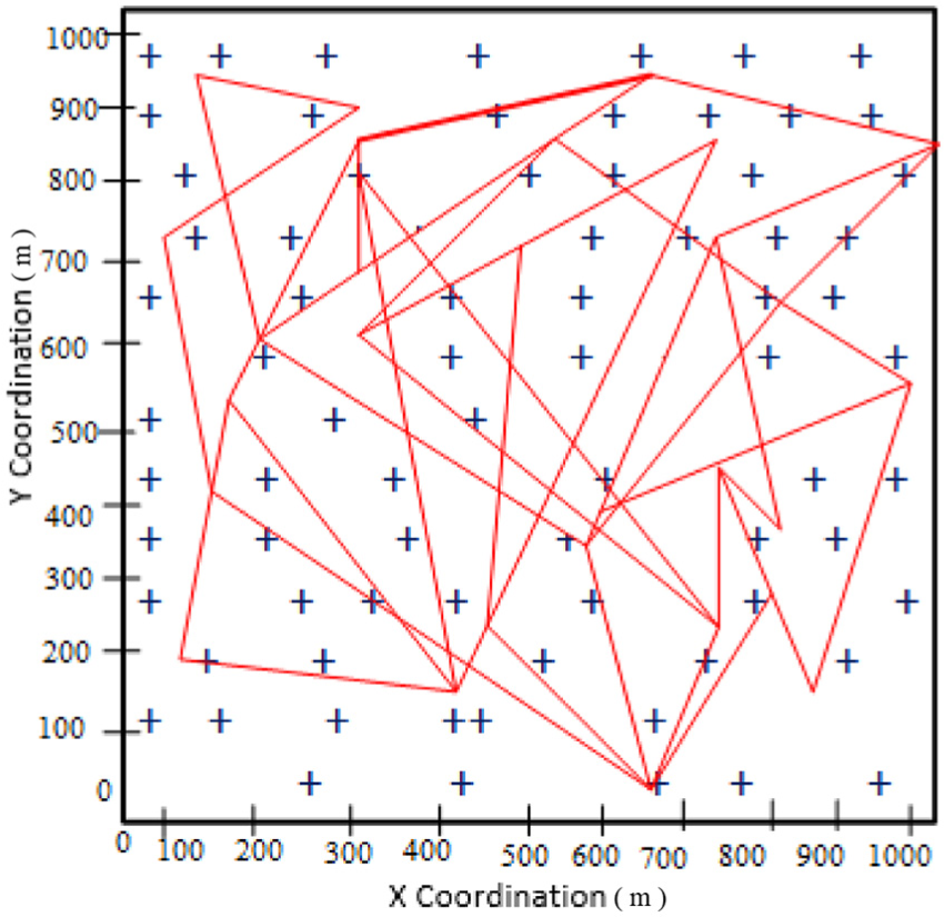
Random way point trajectory of mobile beacon.

Scan

The scan is a simple path planning scheme.⁴¹ The scan can be implemented easily. The traveling trajectory of Scan is shortest. Here, the mobile anchor moves along a single dimension either along x-axis or y-axis as mentioned in Figure 4. One of the advantages of Scan is that it covers the whole network and has lowest localization error. However, Scan has the collinearity issue which mostly occurs due to the movement of mobile beacon in a straight line, which degrades the localization accuracy. Here, the network is divided into $nxn$ sub-squares. The distance between two parallel lines to the Y-axis is defined as resolution denoted by $d$ . The resolution should be small to make sure that all sensors will be able to receive the beacon messages. The resolution should not be more than $d = 2 r$ , where $r$ denotes the communication range. Scan performs best when the distance between the sensor and the unknown node is small. The total distance (Dscan) traversed by the mobile landmark in Scan is calculated by

D_{Scan} = (4^{n} - 1) R

(1)

Figure 4.

Scan trajectory of mobile beacon.

Double Scan

To overcome the collinearity issues, Double Scan traverses the network region along both directions x-axis and y-axis as shown in Figure 5. The collinearity problem is resolved in Double Scan. Double Scan also has a drawback. Here, the path length is doubled; due to this, the energy consumption is also increased. The total distance traversed by the mobile landmark in Double Scan is calculated by

D_{DoubleScan} = (4^{n} + 2^{n} - 4) R

(2)

Figure 5.

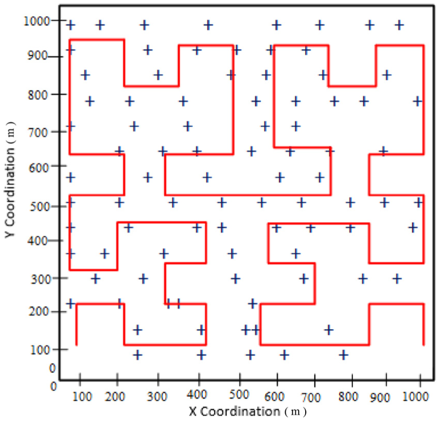
Double Scan trajectory of mobile beacon.

Hilbert

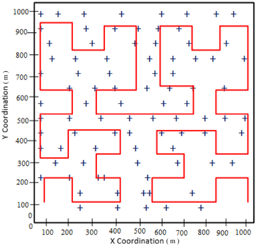
Hilbert makes many turns to minimize the collinearity issues without increasing the path length as shown in Figure 6.⁴¹ However, it also has a potential drawback that is the mobile beacon will never traverse on the corner of the sensing field. The sensor close to the corner will hear beacon points only from one direction, and their estimate will not be authentic. In Hilbert, the whole network is not covered and have higher chances of localization error. Hilbert curve divides the two-dimensional space into the $4^{n}$ square cell and connects the center of those cells using $4^{n}$ line segments. In the equation, $4^{n}$ is the level of Hilbert curve, and $R$ is the resolution of the trajectory. The entire distance traversed by the mobile anchor node in Hilbert is calculated by

D_{Hilbert} = 4^{n} R

(3)

Figure 6.

Hilbert trajectory of mobile beacon.

Circles

Circles path planning algorithm is used to reduce the collinearity issues as shown in Figure 7. Mobile anchor follows circular trajectory instead of a straight line to avoid the collinearity issues. Circle do not cover the whole network effectively. Moreover, Circles has a scalability issue. When the sensing field extends, Circles becomes larger. When circles become larger, collinearity issues raise and hence decreases the localization accuracy. The resolution d is defined as half of the radius of the innermost circle. Dividing the network size into $n \times n$ sub-squares, the total distance traversed by the mobile landmark in Circle can be represented as a function of d and n as follows

D = \frac{n^{2} π R}{4} + (\frac{n}{2} - 1) R

(4)

Figure 7.

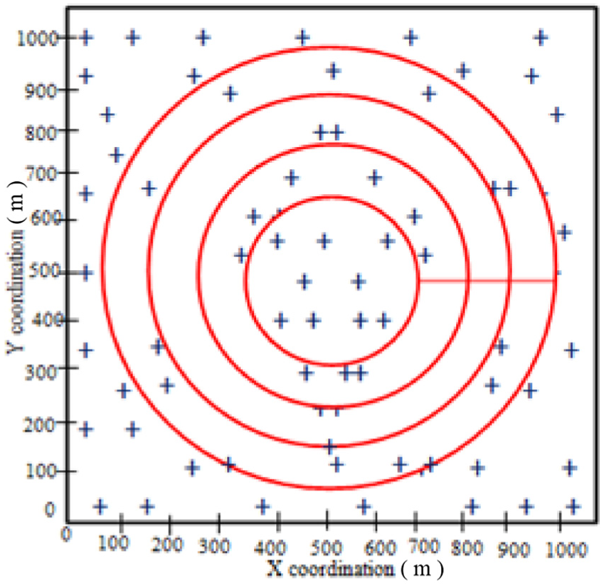
Circle trajectory of mobile beacon.

Results and discussion

In this section, the performance of the four static path planning algorithms and RWP are analyzed using performance analysis parameters such as accuracy, energy consumption, and number of references. Network simulator-2 is used as a simulation tool to implement the path planning algorithm and to design various network simulation scenarios. Three simulation scenarios of unknown sensor nodes such as sparse node density (20 nodes), medium node density (40 nodes), and dense node density (80 nodes) are used. These sensor nodes are randomly deployed in the sensing field with a single mobile beacon around them. The deployment area of the network is set equal to $1000 m^{2}$ . Here, in this scenario, the mobile beacon speed is set to 10 m/s while the simulation time is 1000 s as mentioned in Table 1.

Table 1.

Parameters configuration of simulation scenarios.

Parameter	Value
Simulation area	1000 × 1000 m²
Simulation time	1000 s
Beacon node	1
Beacon speed	10 m/s

Performance analysis parameters

Three performance analysis parameters such as accuracy, energy consumption, and number of reference nodes are used to evaluate the static path planning algorithms. These analysis parameters are used to find the effectiveness of the selected five path planning algorithms as mentioned below.

Location error ratio (accuracy)

Location error is one of the main critical issues in WSN. Localization algorithm and sensor mobility are the main reasons due to which location error occurs. Location error is the average difference between the estimated and actual sensor node location. The average localization error is considered to analyze the accuracy of the estimated locations. The location error for the unknown sensor is calculated by measuring the distance between the actual location of the nodes $(x_{i}, y_{i})$ and its estimated location $(x_{ei}, y_{ei})$ ³⁹ Mathematical formula of the average location error $(L_{e})$ for the total number of n unknown node is mentioned below

L_{e} = \frac{\sum_{i = 1}^{n} Error (i)}{n}

(5)

Erro r_{(i)} = \sqrt{{(x_{ei} - x_{i})}^{2} + {(y_{ei} - y_{i})}^{2}}

(6)

The variable $(x_{ei}, y_{ei})$ is used to represent estimated location of nodes, and the variable $(x_{i}, y_{i})$ is for the actual location of the nodes. The variable $L_{e}$ indicates the location error while $n$ is the number of unknown nodes.

Figure 8 shows the accuracy of path planning algorithms in terms of location error ratio with increasing number of nodes. Hilbert outperforms in sparse node density scenario by having minimum location error ratio. In case of medium and dense node density scenarios, the RWP has lowest location error ratio. RWP has the lowest localization error compared to other trajectories because it moves in a random direction with random speed. RWP has successfully overcome the collinearity issues. Accuracy decreases and location error ratio increases with the increase in the number of nodes. The increased number of nodes impacts both the absolute values for the localization errors and the relative performance of the trajectories.

Figure 8.

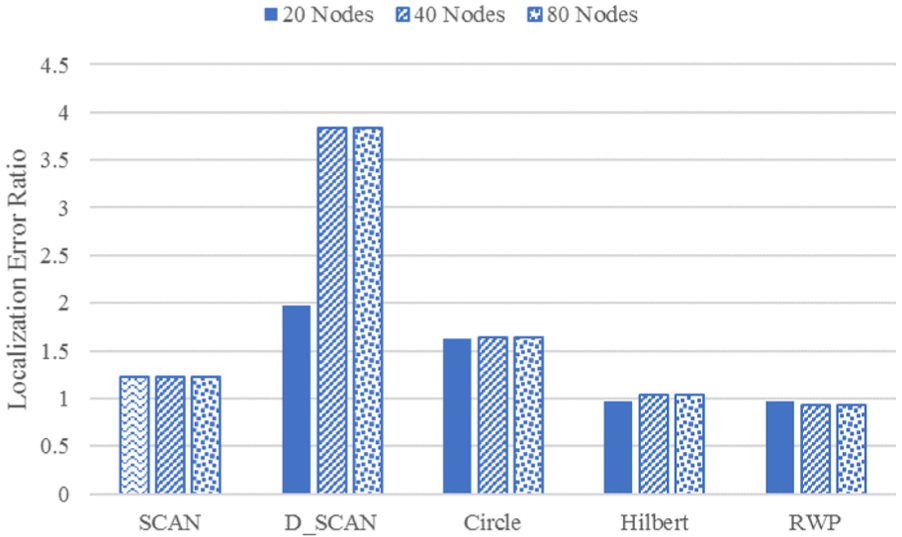
Accuracy (location error ratio) of Scan, D_Scan, Circle, Hilbert, and RWP with increasing number of nodes.

The increase in number of nodes has no significant impact on Scan. Scan covers the whole network. Scan has collinearity issues due to movement of beacon node in straight line. Double Scan has the largest location error compared to another path planning scheme. It is observed that RWP outperforms Scan, Double Scan, and Circle by having lowest localization error.

Energy consumption

Energy consumption is the amount of energy consumed or used by a sensor node during localization. Energy consumption is measured in joules. During localization, the energy is consumed in two ways. In the first case, the energy is consumed by the mobile beacon. In the second situation, energy is consumed by unknown nodes for localization. The mobile beacon energy consumption is divided into two domains: the energy consumption for sending messages $(E_{send})$ and the energy required for traveling along the trajectory $(E_{travel})$ . Unknown nodes also consume energy during localization. Due to a large number of sensors, more energy is consumed which influences the lifetime of the sensor.³⁹ The total energy consumed by both the mobile anchor node and unknown sensors is shown mathematically as

E_{total} = \frac{E_{beacon} + E_{sensor}}{Number of localized sensors}

(7)

Here, the variable E_total denotes the total energy. Energy consumed by mobile beacon and sensor are denoted by E_beacon and E_sensor, respectively.

Figure 9 shows energy consumption of path localization algorithms with respect to sparse, medium, and dense node density scenarios. Hilbert has lowest energy consumption in sparse node density scenario. RWP maintains its minimum energy consumption in medium and dense node density scenarios. SCAN consumes more energy to localize the nodes compared to other trajectories in sparse, medium, and dense node density scenarios.

Figure 9.

Energy consumption of Scan, D_Scan, Circle, Hilbert, and RWP with increasing number of nodes.

Number of references

Localization accuracy of a unknown node improves with the increase in number of references $(R_{n})$ in WSN. This increase in number of references also creates computations complexity. Mathematically, the average number of references $(R_{n})$ is shown as⁵⁸

R_{n} = \frac{1}{n} \sum_{1}^{n} C (S_{i})

(7)

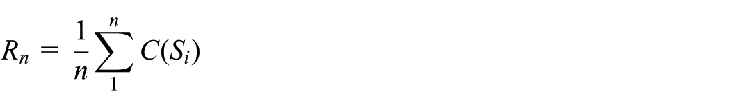
where the total number of localized nodes is $n$ during time t and $S_{i}$ is the total number of references used to localized unknown node $i$ . $C (S_{i})$ is the cardinality of set $S_{i}$ . Figure 10 shows the average number of references used by each algorithm.

Figure 10.

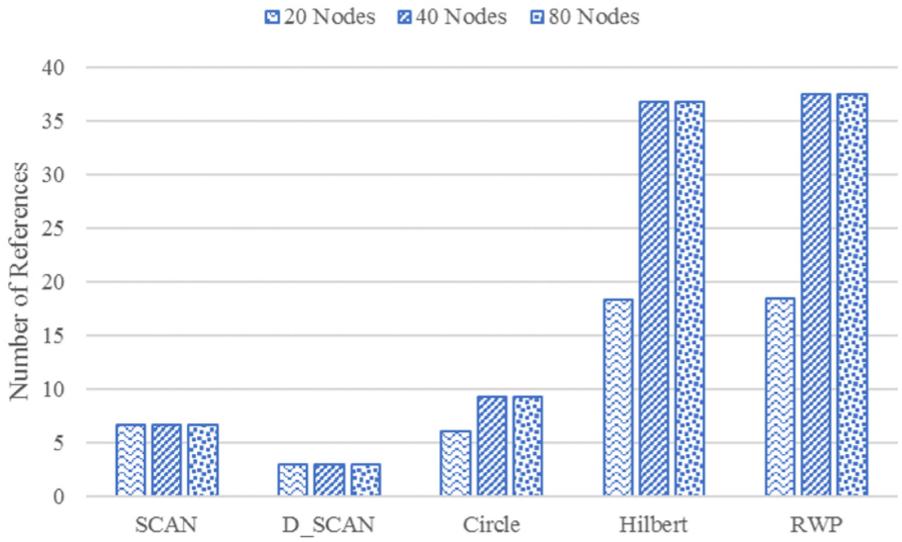
Number of reference nodes of Scan, D_Scan, Circle, Hilbert, and RWP with increasing number of nodes.

Figure 10 shows the average number of references used by static path planning algorithms. RWP outperformed by having a higher number of references in sparse, medium, and dense node density scenarios. D-Scan has the lowest number of references in sparse, medium, and dense node density scenarios. In short, RWP outperformed in medium and dense node density scenarios by having higher accuracy, minimum energy consumption, and higher number of references. Hilbert has comparatively higher accuracy, minimum energy consumption, and higher number of references in sparse node density scenario.

Conclusion

In this article, five path planning schemes, namely, RWP, Scan, D-Scan, Hilbert, and Circles, are evaluated using three performance analysis parameters, that is, location error ratio, energy consumption, and number of references. The simulation results revealed that RWP has comparatively higher performance efficiency in terms location error ratio (accuracy), energy consumption, and number of references in medium and dense node density scenarios. Localization error ratio of RWP in medium and dense node density scenarios is decreased by 52.51% of maximum possible localization error of SCAN. Energy consumption of RWP in medium and dense node density scenarios is decreased by 1.72% of maximum possible energy consumption of SCAN. Number of references of RWP is increased by 1147.66% in medium and dense node density scenarios compared to the number of references of D-SCAN. Hilbert performs well in sparse node density scenario. Hilbert has a decrease of 50.97% in location error ratio compared to location error ratio of SCAN in sparse node density scenario. Energy consumption of Hilbert in sparse node density scenario is decreased by 0.42% of maximum possible energy consumption of SCAN. Number of references of Hilbert is increased by 515.70% in sparse node density scenarios compared to D-SCAN. The performance of localization of a beacon node in RWP can be further improved by avoiding the repeated visit of mobile beacon node to same unknown sensor nodes. In future, it is necessary to handle obstacle-resistant trajectory in the sensing field. There is a need to find the optimal transmission power used by mobile landmark concerning the distance from unknown nodes to enhance the energy efficiency and localization accuracy.

Footnotes

Handling Editor: Gianluigi Ferrari

Declaration of conflicting interests

The author(s) declared no potential conflicts of interest with respect to the research, authorship, and/or publication of this article.

Funding

The author(s) received no financial support for the research, authorship, and/or publication of this article.

References

Liu

Yang

Wang

et al . Location, localization, and localizability. J Comput Sci Technol 2010; 25(2): 274–297.

Ahmed

Kanhere

Jha

. The holes problem in wireless sensor networks: a survey. ACM SIGMOBILE Mob Comput Commun 2005; 9(2): 4–18.

Katiyar

Chand

Soni

. A survey on clustering algorithms for heterogeneous wireless sensor networks. Int J Adv Netw Appl 2011; 2(4): 745–754.

Akyildiz

Sankarasubramaniam

et al . Wireless sensor networks: a survey. Comput Netw 2002; 38(4): 393–422.

Maraiya

Kant

Gupta

. Application based study on wireless sensor network. Int J Comput Appl 2011; 21(8): 9–15.

Arampatzis

Lygeros

Manesis

. A survey of applications of wireless sensors and wireless sensor networks. In: Proceedings of the intelligent control and international symposium on, Mediterranean conference on control and automation, Limassol, Cyprus, 27–29 June 2005, pp.719–724. New York: IEEE.

Huang

Záruba

. Monte Carlo localization of wireless sensor networks with a single mobile beacon. Wirel Netw 2009; 15(8): 978–990.

Perrig

Szewczyk

Tygar

et al . SPINS: security protocols for sensor networks. Wirel Netw 2002; 8(5): 521–534.

Xiang

Luo

Vasilakos

. Compressed data aggregation for energy efficient wireless sensor networks. In: Proceedings of the 8th annual communications society conference on sensor, mesh and ad hoc communications and networks, Salt Lake City, UT, 27–30 June 2011, pp.46–54. New York: IEEE.

10.

Lin

Chen

. Improving the coverage of randomized scheduling in wireless sensor networks. IEEE T Wirel Commun 2008; 7(12): 4807–4812.

11.

Zeng

Xiang

et al . Directional routing and scheduling for green vehicular delay tolerant networks. Wirel Netw 2013; 19(2): 161–173.

12.

Sheng

Yang

et al . A survey on the IETF protocol suite for the Internet of Things: standards, challenges, and opportunities. IEEE Wirel Commun 2013; 20(6): 91–98.

13.

Zeng

Cao

Hong

et al . Secure localization and location verification in wireless sensor networks: a survey. J Supercomput 2013; 64(3): 685–701.

14.

Han

Duong

et al . Localization algorithms of wireless sensor networks: a survey. Telecommun Syst 2013; 52(4): 2419–2436.

15.

Kumar

Lobiyal

. Power efficient range-free localization algorithm for wireless sensor networks. Wirel Netw 2014; 20(4): 681–694.

16.

Camp

Boleng

Davies

. A survey of mobility models for ad hoc network research. Wirel Commun Mob Comput 2002; 2(5): 483–502.

17.

Halder

Ghosal

. A survey on mobile anchor assisted localization techniques in wireless sensor networks. Wirel Netw 2016; 22(7): 2317–2336.

18.

Stoleru

Stankovic

. Probability grid: a location estimation scheme for wireless sensor networks. In: Proceedings of the 1st annual communications society conference on sensor and ad hoc communications and networks, Santa Clara, CA, 4–7 October 2004, pp.430–438. New York: IEEE.

19.

Huang

Blum

et al . Range-free localization schemes for large scale sensor networks. In: Proceedings of the 9th annual international conference on mobile computing and networking, San Diego, CA, 14–19 September 2003, pp.1–16. New York: ACM.

20.

Shang

Ruml

. Improved MDS-based localization. In: Proceedings of the 23rd annual joint conference of the IEEE computer and communications societies, Hong Kong, China, 7–11 March 2004, pp.2640–2651. New York: IEEE.

21.

Lee

Kim

et al . Localization with a mobile beacon based on geometric constraints in wireless sensor networks. IEEE T Wirel Commun 2009; 8(12): 5801–5805.

22.

Qian

H-Y

. Localization of wireless sensor networks with a mobile beacon. Inf Technol J 2013; 12(11): 2251–2255.

23.

. Path planning algorithm for mobile anchor-based localization in wireless sensor networks. IEEE Sens J 2013; 13(2): 466–475.

24.

Galstyan

Krishnamachari

Lerman

et al . Distributed online localization in sensor networks using a moving target. In: Proceedings of the 3rd international symposium on information processing in sensor networks, Berkeley, CA, 27 April 2004, pp.1–16. New York: IEEE.

25.

Corke

Peterson

Rus

. Networked robots: flying robot navigation using a sensor net. In: Dario

Chatila

(eds) Robotics research. The 11th international symposium (Springer tracts in advanced robotics). Berlin: Springer, 2005, pp.234–243.

26.

Han

Lee

et al . Node distribution-based localization for large-scale wireless sensor networks. Wirel Netw 2010; 16(5): 1389–1406.

27.

Salih

Wang

C-X

et al . Deterministic process-based generative models for characterizing packet-level bursty error sequences. Wirel Commun Mob Comput 2015; 15: 421–430.

28.

Rezazadeh

Moradi

Ismail

. Message-efficient localization in mobile wireless sensor networks. J Comm Comput 2012; 9: 340–344.

29.

Shu

Zhang

Liu

et al . Cluster-based three-dimensional localization algorithm for large scale wireless sensor networks. J Comput 2009; 4(7): 585–592.

30.

Rezazadeh

Moradi

Ismail

. Mobile wireless sensor networks overview. Int J Comput Commun Netw 2012; 2(1): 17–22.

31.

Halder

Ghosal

. A survey on mobility-assisted localization techniques in wireless sensor networks. J Netw Comput Appl 2016; 60: 82–94.

32.

Patwari

Ash

Kyperountas

et al . Locating the nodes: cooperative localization in wireless sensor networks. IEEE Signal Process Mag 2005; 22(4): 54–69.

33.

Rezazadeh

Moradi

. Efficient localization via middle-node cooperation in wireless sensor networks. Int Conf Electr Control Comput Eng 2011; 2011: 410–415.

34.

Patwari

Hero

Perkins

et al . Relative location estimation in wireless sensor networks. IEEE T Signal Proces 2003; 51(8): 2137–2148.

35.

Chang

T-C

Wang

Hsieh

Y-L

. Enhanced color-theory-based dynamic localization in mobile wireless sensor networks. In: Proceedings of the wireless communications and networking conference, Kowloon, China, 11–15 March 2007, pp.3064–3069. New York: IEEE.

36.

Chen

Shi

Tan

et al . Mobile element assisted cooperative localization for wireless sensor networks with obstacles. IEEE T Wirel Commun 2010; 9(3): 956–963.

37.

Ssu

Jiau

. Localization with mobile anchor points in wireless sensor networks. IEEE T Veh Technol 2005; 54(3): 1187–1197.

38.

Wang

Zhu

. Sequential Monte Carlo localization in mobile sensor networks. Wirel Netw 2007; 15(4): 481–495.

39.

Rezazadeh

Moradi

Ismail

et al . Impact of static trajectories on localization in wireless sensor networks. Wirel Netw 2015; 21(3): 809–827.

40.

Zhong

Luo

D-Y

Liu

S-Q

et al . An adaptive localization approach for wireless sensor networks based on Gauss-Markov mobility model. Acta Autom Sin 2010; 36(11): 1557–1568.

41.

Koutsonikolas

Das

. Path planning of mobile landmarks for localization in wireless sensor networks. Comput Commun 2007; 30(13): 2577–2592.

42.

Taylor

Bahi

Makhoul

et al . Hilbert mobile beacon for localization and coverage in sensor networks. Int J Syst Sci 2008; 39(11): 37–41.

43.

Bahi

Makhoul

Mostefaoui

. Localization and coverage for high density sensor networks. Comput Commun 2008; 31(4): 770–781.

44.

Huang

Záruba

. Static path planning for mobile beacons to localize sensor networks. In: Proceedings of the 5th annual international conference on pervasive computing and communications workshops, White Plains, NY, 19–23 March 2007, pp.323–328. New York: IEEE.

45.

Song

et al . Localization in wireless sensor networks using a mobile anchor node. In: Proceedings of the IEEE/ASME international conference on advanced intelligent mechatronics, Xi’an, China, 2–5 July 2008, pp.602–607. New York: IEEE.

46.

Priyantha

Balakrishnan

Demaine

et al . Mobile-assisted localization in wireless sensor networks. In: Proceedings of the 24th annual joint conference of the IEEE computer and communications societies, Miami, FL, 13–17 March 2005, pp.172–183. New York: IEEE.

47.

Benkhelifa

Moussaoui

. APPL: anchor path planning based localization for wireless sensor networks. In: Proceedings of the 4th international conference on communications, computers and applications, Istanbul, Turkey, July 2011, pp.48–53. Istanbul: Mosharaka for Researches and Studies.

48.

Cui

Wang

Cuia

et al . Path planning of mobile anchor in three-dimensional wireless sensor networks for localization. J Inform Comput Sci 2012; 8(8): 2203–2210.

49.

Han

Jiang

et al . Path planning using a mobile anchor node based on trilateration in wireless sensor networks. Wirel Commun Mob Comput 2013; 13(14): 1324–1336.

50.

Han

Zhang

Lloret

et al . A mobile anchor assisted localization algorithm based on regular hexagon in wireless sensor networks. Sci World J 2014; 2014: 1–13.

51.

C-H

. Localization of wireless sensor networks using a single anchor node. IEEE Sens J 2011; 11(7): 1607–1616.

52.

Rezazadeh

Moradi

Ismail

et al . Superior path planning mechanism for mobile beacon-assisted localization in wireless sensor networks. IEEE Sens J 2014; 14(9): 3052–3064.

53.

Han

Yang

Liu

et al . A disaster management-oriented path planning for mobile anchor node-based localization in wireless sensor networks. IEEE Trans Emerg Top Comput 2017; 1–12. DOI: 10.1109/TETC.2017.2687319.

54.

Han

Zhang

Jiang

et al . Mobile anchor nodes path planning algorithms using network-density-based clustering in wireless sensor networks. J Netw Comput Appl 2017; 85: 64–75.

55.

Alomari

Comeau

Phillips

et al . New path planning model for mobile anchor-assisted localization in wireless sensor networks. Wirel Netw 2017; 1–19. DOI: https://doi.org/10.1007/s11276-017-1493-2.

56.

Kong

Lowe

. Dynamic path determination of mobile beacons employing reinforcement learning for wireless sensor localization. In: Proceedings of the 26th international conference on advanced information networking and applications workshops, Fukuoka, Japan, 26–29 March 2012, pp.760–765. New York: IEEE.

57.

Hongjun

Jianwen

Xun

et al . Real-time path planning of mobile anchor node in localization for wireless sensor networks. In: Proceedings of the international conference on information and automation, Changsha, China, 20–23 June 2008, pp.384–389. New York: IEEE.

58.

Abu-Mahfouz

Hancke

Isaac

. Positioning system in wireless sensor networks using NS-2. Softw Eng 2012; 2(4): 91–100.

On precise path planning algorithm in wireless sensor network

Abstract

Keywords

Introduction

Related work

Mobile beacon trajectory

Static path planning

Dynamic path planning

Static path planning of mobile beacon for localization

RWP

Scan

Double Scan

Hilbert

Circles

Results and discussion

Performance analysis parameters

Location error ratio (accuracy)

Energy consumption

Number of references

Conclusion

Footnotes

Declaration of conflicting interests

Funding

References