Sage Journals: Discover world-class research

Abstract

This paper reviews some of the recent advances in the development of algorithms for wireless sensor networks. We focus on sensor deployment and coverage, routing, and sensor fusion.

Keywords

Wireless sensor networks algorithms routing coverage fusion

1. Introduction

A wireless sensor network may comprise thousands of sensor nodes. Each sensor node has a sensing capability as well as limited energy supply, compute power, memory, and communication ability. Besides military applications, wireless sensor networks may be used to monitor microclimates and wildlife habitats [45], the structural integrity of bridges and buildings, buildings security, location of valuable assets (via sensors placed on these valuable assets), traffic, and so on. However, realizing the full potential of wireless sensor networks poses myriad research challenges ranging from hardware and architectural issues, to programming languages and operating systems for sensor networks, to security concerns, to algorithms for sensor network deployment, operation, and management. Iyengar and Brooks [20], [21] and Culler and Hong [8] provide good overviews of the breadth of sensor network research topics as well as of applications for sensor networks.

This paper focuses on some of the algorithmic issues that arise in the context of wireless sensor networks. Specifically, we review algorithmic issues in sensor deployment and coverage, routing, and fusion. There is an abundance of algorithmic research related to wireless sensor networks. At a high level, the developed algorithms may be categorized as either centralized or distributed. Because of the limited memory, compute, and communication capability of sensors, distributed algorithms research has focused on localized distributed algorithms—distributed algorithms that require only local (e.g., nearest neighbor) information.

2. Sensor Deployment and Coverage

In a typical sensor network application, sensors are to be placed (or deployed) so as to monitor a region or a set of points. In some applications, we may be able to select the sites where sensors are placed, while in others (e.g., in hostile environments), we may simply scatter (e.g., airdrop) a sufficiently large number of sensors over the monitoring region with the expectation that the sensors that survive the airdrop will be able to adequately monitor the target region. When site selection is possible, we use deterministic sensor deployment, and when site selection is not possible, the deployment is nondeterministic. In both cases, it is often desirable that the deployed collection of sensors be able to communicate with one another, either directly or indirectly via multihop communication. So, in addition to covering the region or set of points to be sensed, we often require the deployed collection of sensors to form a connected network. For a given placement of sensors, it is easy to check whether the collection covers the target region or point set and also whether the collection is connected. For the coverage property, we need to know the sensing range of individual sensors. (We assume that a sensor can sense events that occur within a distance r, where r is the sensor's sensing range.) For the connected property, we need to know the communication range, c, of a sensor. Zhang and Lou [60] have established the following necessary and sufficient condition for coverage to imply connectivity.

Theorem 1

(Zhang and Lou [60]) When the sensor density (i.e., number of sensors per unit area) is finite, c ≥ 2r is a necessary and sufficient condition for coverage to imply connectivity.

Wang et al. [49] prove a similar result for the case of k-coverage (each point is covered by at least k sensors) and k-connectivity (the communication graph for the deployed sensors is k connected).

Theorem 2

(Wang et al. [49]) When c ≥ 2r, k-coverage of a convex region implies k-connectivity.

Notice that k-coverage with k > 1 affords some degree of fault tolerance. We are able to monitor all points so long as no more than k − 1 sensors fail. Huang and Tseng [19] develop algorithms to verify whether a sensor deployment provides k-coverage. Other variations of the sensor deployment problem are also possible. For example, we may have no need for sensors to communicate with one another. Instead, each sensor communicates directly with a base station that is situated within the communication range of all sensors. In another variant [17], [18], the sensors are mobile and self-deploy. A collection of mobile sensors may be placed into an unknown and potentially hazardous environment. Following this initial placement, the sensors relocate so as to obtain maximum coverage of the unknown environment. They communicate the information they gather to a base station outside of the environment being sensed. A distributed potential-field-based algorithm to self-deploy mobile sensors under the stated assumptions is developed in [18], and a greedy and incremental self-deployment algorithm is developed in [17]. A virtual-force algorithm to redeploy sensors so as to maximize coverage is developed by Zou and Chakrabarty [61]. Poduri and Sukhatme [38] developed a distributed self-deployment algorithm that is based on artificial potential fields and that maximizes coverage while ensuring that each sensor has at least k other sensors within its communication range.

2.1 Deterministic Deployment

2.1.1 Region Coverage

Kar and Banerjee [25] examined the problem of deploying the fewest number of homogeneous sensors so as to cover the plane with a connected sensor network. They assumed that the sensing range equals the communication range (i.e., r = c). Figure 1 gives their deployment algorithm. One may verify that the sensors deployed in Step 1 are able to sense the entire plane. So, these sensors satisfy the coverage requirement. However, the sensors placed in Step 1 define many rows of connected sensors with the property that two sensors in different rows are unable to communicate (i.e., there is no multihop path between the sensors such that adjacent sensors on this path are at most c apart). Step 2 creates a connected network by placing a column of sensors in such a way as to connect the connected rows that result from Step 1.

Figure 1

Kar and Banerjee's [25] sensor-deployment algorithm.

Kar and Banerjee [25] have shown that their algorithm of Fig. 1 has a sensor density that is within 2.6% of the optimal density. This algorithm may be extended to provide connected coverage for a set of finite regions [25].

2.1.2 Point Coverage

Figure 2 gives the greedy algorithm of Kar and Banerjee [25] to deploy a connected sensor network so as to cover a set of points in Euclidean space. This algorithm, which assumes that r = c, uses at most 7.256 times the minimum number of sensors needed to cover the given point set [25]. It is easy to see that the constructed deployment covers all of the given points and is a connected network.

Figure 2

Greedy algorithm of [25] to deploy sensors.

Grid coverage is another version of the point coverage problem. In this version, Chakrabarty et al. [5], we are given a two- or three-dimensional grid of points that are to be sensed. Sensor locations are restricted to these grid points, and each grid point is to be covered by at least m, m ≥ 1, sensors (i.e., we seek m-coverage). For sensing, we have k sensor types available. A sensor of type i costs c_i dollars and has a sensing range r_i. At most, one sensor may be placed at a grid point. In this version of the point coverage problem, the sensors do not communicate with one another and are assumed to have a communication range large enough to reach the base station from any grid position. So, network connectivity is not an issue. The objective is to find a least-cost sensor deployment that provides m-coverage.

Chakrabarty et al. [5] formulated this m-coverage deployment problem as an integer linear program (ILP) with O(kn²) variables and O(kn²) equations, where n is the number of grid points. Xu and Sahni [54] reduce the number of variables to O(kn) and the number of equations to O(n). Also, their formulation does not require the sensor locations and points to be sensed to form a grid. Let s_ij be a 0/1-valued variable with the interpretation s_ij = 1 iff a sensor of type i is placed at point j, 1 ≤ i ≤ k, 1 ≤ j ≤ n. The solution to the following ILP describes an optimal sensor deployment.

\begin{aligned} minimize \sum_{i = 1}^{k} (c_{i} \sum_{j = 1}^{n} s_{i j}) \\ \sum_{i = 1}^{k} \sum_{a \in X (i, j)} s_{i a} \geq m, 1 \leq j \leq n \\ \sum_{i = 1}^{k} s_{i j} \leq 1, 1 \leq j \leq n \end{aligned}

where X(i,j) = {all points within r_i of point j}.

Even with this reduction in the number of variables and equations, the ILP is practically solvable only for a small number of points n. For large n, Chakrabarty et al. [5] proposed a divide-and-conquer “near-optimal” algorithm in which the base case (small number of points) is solved optimally using the ILP formulation.

2.2 Maximizing Coverage Lifetime

When sensors are deployed in difficult-to-access environments, as is the case in many military applications, a large number of sensors may be airdropped into the region that is to be sensed. Assume that the sensors that survive the airdrop cover all targets that are to be sensed. Because the power supply of a sensor cannot be replenished, a sensor becomes inoperable once it runs out of energy. Define the life of a sensor network to be the earliest time at which the network ceases to cover all targets. The life of a network can be increased if it is possible to put redundant sensors (i.e., sensors not needed to provide coverage of all targets) to “sleep” and awaken these sleeping sensors when they are needed to restore target coverage. Sleeping sensors are inactive, while sensors that are awake are active. Inactive sensors consume far less energy than active ones.

Cardei and Du [3] proposed partitioning the set of available sensors into disjoint sets such that each set covers all targets. Let T be the set of targets to be monitored, and let Si denote the subset of T in the range of sensor i, 1 ≤ i ≤ n. Let P₁, P₂, …, P_k be disjoint partitions of the set of n sensors such that $\cup_{j \in P_{i}} S_{j} = T, 1 \leq i \leq k$ . Then, the set of sensors in each P_i covers all targets. We refer to the set of P_is as a disjoint set cover of size k. Moreover, by going through k sleep/awake rounds, where in round i only the sensors in P_i are awake, we are able to monitor all targets in each round and increase the network life to almost kt, where t is the time it takes a sensor to deplete its energy when in the awake mode. Because sensors deplete energy even when in the sleep mode, the life of each round is slightly less than that of the preceding round. Cardei and Du [3] have shown that deciding whether there is a disjoint set cover of size k for a given sensor set is NP-complete. They develop a heuristic to maximize the size of a disjoint set cover. An experimental evaluation of this heuristic reveals that it finds about 10% more disjoint covers than does the best algorithm of Slijepcevic and Potkonjak [43]. However, the algorithm of Cardei and Du [3] takes more time to execute.

Several decentralized localized protocols to control the sleep/awake state of sensors so as to increase network lifetime have been proposed. Ye, Zhong, Lu, and Zhang [58] proposed a simple protocol. In this protocol, the set of active nodes provides the desired coverage. A sleeping node wakes up when its sleep timer expires, and it broadcasts a probing signal a distance d (d is called the probing range). If no active sensor is detected in this probing range, the sensor moves into the active state. However, if an active sensor is detected in the probing range, the sensor determines how long to sleep, sets its sleep timer, and goes to sleep. Techniques to dynamically control the sleep time and probing range are discussed in [58]. Simulations reported in [58] indicate that this simple protocol outperforms the GAF protocol of [55]. However, experiments conducted by Tian and Georganas [46] reveal that the protocol of Ye et al. [58] “cannot ensure the original sensing coverage and blind spots may appear after turning off some nodes.” Tian and Georganas [46] proposed an alternative distributed localized protocol that sensors may use to turn themselves on and off. The network operates in rounds, where each round has two phases—self-scheduling and sensing. In the self-scheduling phase, each sensor decides whether or not to go to sleep. In the sensing phase, the active/awake sensors monitor the region. Sensor s turns itself off in the self-scheduling phase if its neighbors are able to monitor the entire sensing region of s. To make this determination, every sensor broadcasts its location and sensing range. A back-off scheme is proposed to avoid blind spots that would otherwise occur if two sensors turn off simultaneously, each expecting the other to monitor part or all of its sensing region. In this back-off scheme, each active sensor uses a random delay before deciding whether or not it can go to sleep without affecting sensing coverage.

The decentralized algorithm OGDC (optimal geographical density control) of Zhang and Hou [60] guarantees coverage, which by Theorem 1 implies connectivity, whenever the sensor communication range is at least twice its sensing range. Experimental results reported in [60] suggest that when OGDC is used, the number of active (awake) nodes may be up to half that when the PEAS [57] or GAF [55] algorithms are used to control sensor state. The Coverage Configuration Protocol (CCP) to maximize lifetime while providing k-coverage (as well as k-connectivity when c ≥ 2r, Theorem 2) is developed in [49]. A distributed protocol for differentiated surveillance is proposed by Yan, He, and Stankovic [56].

Assume that the probability that sensor s detects an event at a distance d is P(s,x) = 1/(1 + αd)^β. The probability P(x) that an event at x is detected by the sensor network is

P (x) = 1 - Π (1 - P (s, x))

where the product is taken over all sensors in the network. The coverage, C, of the sensor network (overall network coverage) is the sum of P(x) over all points in the sensing region. Let C′(s) be the overall coverage when sensor s is removed from the network. The sensing denomination [29] of a sensor s is its contribution, C - C′(s), to overall network coverage. Lu and Tatsuya [29] use the sensing denomination of a sensor to obtain a distributed localized self-scheduling algorithm to schedule the sleep/awake states of sensors so as to increase network lifetime. In their algorithm, each sensor periodically makes a decision to either go to sleep or be active. Sensors with higher sensing denominations have a higher probability of being active.

2.3 Deployment Quality

The quality of a sensor deployment may be measured by the minimum k for which the deployment provides k-coverage as well as by the minimum k for which we have k-connectivity. By Theorem 2, the first metric implies the second when the communication range c is at least twice the sensing range r. Meguerdichian et al. [33] formulated additional metrics suitable for a variety of sensor applications. In these applications, the ability of a sensor to detect an activity a distance d from the sensor is given by the function α/(1 + d),^β where α and β are constants. So, sensing ability is at a maximum when d = 0 and declines as we get farther from the sensor.

Let P be a path that connects two points u and v. (These points may be within or outside the region being sensed.) The breach weight, BW(P, u, v), of P is the closest path P gets to any of the deployed sensors. The breach weight, BW(u, v), of the points u and v is the maximum of the breach weights of all paths between u and v:

B W (u, v) = max {B W (P, u, v) ∣ P is a path between u and v}

The breach weight or breachability, BW, of a sensor network is the maximum of the breach weights of all point pairs:

B W = max {B W (u, v) ∣ u and v are points on the boundary of the sensing region}

When the ability of a sensor to detect an activity is inversely proportional to some power k of distance, sensor deployments that minimize breach weight are preferred. The breachability of a network gives us an indication of how successful an intruder could be in evading detection. Suppose we have an application in which items are being transported between pairs of points, and our sensors track the progress of these shipments. Now we wish to use maximally observable paths, that is, paths that remain as close to a sensor as possible. Let d(x) be the distance between a point x and the sensor nearest to x. Meguerdichian et al. [33] define the support weight, SW(P, u, v), of a path P between u and v as

S W (P, u, v) = max {d (x) ∣ x is a point on P}

SW(u, v) is now defined as

S W (u, v) = min {S W (P, u, v) ∣ P is a path between u and v}

and the support weight (or simply support), SW, of the sensor network is

S W = max {S W (u, v) ∣ u and v are points on the boundary of the sensing region}

Although Meguerdichian et al. [33] developed centralized algorithms to compute BW(u, v) and SW(u, v), these algorithms are flawed [28]. Li, Wan and Frieder [28] described a distributed localized algorithm to determine SW(u, v). This algorithm is given in Fig. 3. In this algorithm, |sa| is the Euclidean distance between the sensors s and a. The algorithm assumes that u and v are in the convex hull of the sensor locations.

Figure 3

Distributed algorithm of [28] to compute SW(u, v).

Because there may be several paths with the computed SW(u, v) value, we may be interested in finding, say, a best support path from u to v that has minimal length. Li et al. [28] developed a localized distributed algorithm to find an approximately minimal length path with support SW(u, v).

The exposure E(P, u, v) of a path P from u to v is defined as

E (P, u, v) = \int_{u}^{v} S (x) d x

where S(x) is a sensing function, and the integral is computed over the path P. Meguerdichian et al. [34] suggested two sensing functions. One is simply the sensing ability of the closest sensor to x; the other is the sum of the abilities of all sensors to detect activity at x. An intruder who wishes to minimize the risk of detection would take a minimal exposure path to get from u to v. Figure 4 gives the algorithm of [34] to find an approximation to the minimal-exposure path between u and v. This algorithm overlays an undirected weighted graph over the sensing region and then finds a shortest path from the graph vertex nearest to u to the graph vertex nearest to v. This shortest path may be found using Dijkstra's shortest-path algorithm. By increasing the number of vertices and edges used in Step 1, the accuracy of the approximation is increased. For the overlay graph, [34] considers a uniform two-dimensional grid arrangement of the vertices and a variety of options for edges (e.g., edges connect a vertex to its north, south, east, west, northwest, northeast, southeast, and southwest neighbors). Sensor deployments that maximize minimal-exposure are preferred.

Figure 4

Algorithm of [34] to find an approximate minimal-exposure path.

Veltri et al. [47] developed a distributed localized algorithm to find an approximate minimal-exposure path. Also, they showed that finding a maximal-exposure path is NP-hard, and they proposed several heuristics to construct approximate maximal-exposure paths. Additionally, a linear programming formulation for minimal- and maximal-exposure paths was obtained. Kanan et al. [23] developed polynomial time algorithms to compute the maximum vulnerability of a sensor deployment to attack by an intelligent adversary, and they used this to compute optimal deployments with minimal vulnerability.

3. Routing

Traditional routing algorithms for sensor networks are datacentric in nature. Given the unattended and untethered nature of sensor networks, datacentric routing must be collaborative as well as energy-conserving for individual sensors. Kannan et al. [22], [24] have developed a novel sensor-centric paradigm for network routing using game theory. In this sensor-centric paradigm, the sensors collaborate to achieve common network-wide goals, such as route reliability and path length, while minimizing individual costs. The sensor-centric model can be used to define the quality of routing paths in the network (also called path weakness). Kannan et al. [24] described inapproximability results on obtaining paths with bounded weakness along with some heuristics for obtaining strong paths. The development of efficient distributed algorithms for approximately optimal strong routing is an open issue that can be explored further.

Energy conservation is an overriding concern in the development of any routing algorithm for wireless sensor networks. This is because such networks are often located where it is difficult, if not impossible, to replenish the energy supply of a sensor. Three forms—unicast, broadcast, and multicast—of the routing problem have received significant attention in the literature. The overall objective of these algorithms is to maximize the lifetime (earliest time at which a communication fails) or the capacity of the network (amount of data traffic carried by the network over some fixed period of time).

Assume that the wireless network is represented as a weighted directed graph G that has n vertices/nodes and e edges. Each node of G represents a node of the wireless network. The weight w(i,j) of the directed edge (i,j) is the amount of energy needed by node i to transmit a unit message to node j.

In the most common model used for power attenuation, signal power attenuates at the rate a/r^d, where a is a media-dependent constant, r is the distance from the signal source, and d is another constant between two and four [39]. So, for this model, w(i, j) = w(j, i) = c ∗ r(i, j)^d, where r(i,j) is the Euclidean distance between nodes i and j, and c is a constant. In practice, however, this nice relationship between w(i,j) and r(i,j) may not apply. This may, for example, be due to obstructions between the nodes that may cause the attenuation to be larger than predicted. Also, the transmission properties of the media may be asymmetric, resulting in w(i, j) ≠ w(j, i).

3.1 Unicast

In a unicast, we wish to send a message from a source sensor s to a destination sensor t. Singh, Woo, and Raghavendra [42] proposed five strategies that may be used in the selection of the routing path for this transmission. The first of these is to use a minimum-energy path (i.e., a path in G for which the sum of the edge weights is minimum) from s to t. Such a path may be computed using Dijkstra's shortest-path algorithm [40]. However, because, in practice, messages between several pairs of source–destination sensors need to be routed in succession, using a minimum-energy path for a message may prevent the successful routing of future messages. As an example, consider the graph of Fig. 5. Suppose that sensors x, b₁, …, b_n initially have 10 units of energy each and that u₁, …, u_n each have one unit. Assume that the first unicast is a unit-length message from x to y. There are exactly two paths from x to y in the sensor network of Fig. 5. The upper path, which begins at x, goes through each of the u_is, and ends at y, uses n + 1 energy units; the lower path uses 2(n + 1) energy units. Using the minimum-energy path depletes the energy in node u_i, 1 ≤ i ≤ n. Following the unicast, sensors u₁, …, u_n are unable to forward any messages. So, an ensuring request to unicast from u_i to u_j, i < j will fail. On the other hand, had we used the lower path, which is not a minimum-energy path, we would not deplete the energy in any sensor, and all unit-length unicasts that could be done in the initial network also can be done in the network following the first x to y unicast.

Figure 5

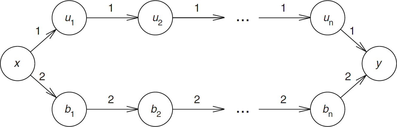
A sensor network.

The remaining four strategies proposed in [42] attempt to overcome the myopic nature of the minimum-energy-path strategy, which sacrifices network lifetime and capacity in favor of total remaining energy. Because routing decisions must be made in an online fashion (i.e., if the ith message is to be sent from s_i to t_i, the path for message i must be decided without knowledge of s_j and t_j, j > i), we seek an online algorithm with a good competitive ratio. It is easy to see that there can be no online unicast algorithm with constant competitive ratio with respect to network lifetime and capacity [1]. For example, consider the network of Fig. 5. Assume that the energy in each node is one unit. Suppose that the first unicast is from x to y. Without knowledge of the remaining unicasts, we must select either the upper or lower path from x to y. If the upper path is chosen and the source–destination pairs for the remaining unicasts turn out to be (u₁, u₂), (u₂, u₃), …, (u_n−1, u_n), (u_n, y), then the online algorithm routes only the first unicast, whereas an optimal off-line algorithm would route all n + 1 unicasts, giving a competitive ratio of n + 1. The same ratio results when the lower path is chosen and the source–destination pairs for the remaining unicasts are (b₁, b₂), (b₂, b₃), …, (b_n−1, b_n), (b_n, y).

Theorem 3

There is no online algorithm to maximize lifetime or capacity that has a competitive ratio smaller than Ω(n).

To maximize lifetime and capacity, we need to achieve some balance between the energy consumed by a route and the minimum residual energy at the nodes along the chosen route. Aslam, Li, and Rus [1] proposed the max–min zP_min-path algorithm to select unicast routes that attempt to make this balance. This algorithm selects a unicast path that uses, at most, z ∗ P_min energy, where z is a parameter to the algorithm, and P_min is the energy required by the minimum-energy unicast path. The selected unicast path maximizes the minimum residual energy fraction (energy remaining after unicast/initial energy) for nodes on the unicast path. Notice that the possible values for the residual energy fraction of node u may be obtained by computing (ce(u) – w(u, v) ∗ l)/ie(u), where l is the message length, ce(u) is the (current) energy at node u just before the unicast, ie(u) is the initial energy at u, and w(u, v) is the energy needed to send a unit-length message along the edge (u, v). This computation is done for all vertices v adjacent from u. Hence, the union, L, of these values taken over all u gives the possible values for the minimum residual-energy fraction along any unicast path. Figure 6 gives the max–min zP_min algorithm.

Figure 6

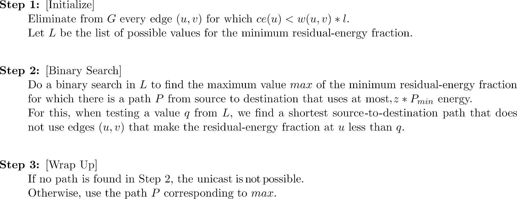
The max–min zP_min unicast algorithm of [11].

Several adaptations to the basic max–min zP_min algorithm, including a distributed version, are described in [1]. Kar et al. [42] developed an online capacity-competitive algorithm, CMAX, with a logarithmic competitive ratio. On the surface, this would appear to violate Theorem 3. However, to achieve this logarithmic competitive ratio, the algorithm CMAX does admission control. That is, it rejects some unicasts that are possible. The bound of Theorem 3 applies only for online algorithms that must perform every unicast that is possible.

Let ce, E, and l be as for the max–min zP_min algorithm. Let α(u) = 1 – ce(u)/ie(u) be the fraction of u's initial energy that has been used so far. Let λ and σ be two constants. In the CMAX algorithm, the weight of every edge (u, v) is changed from w(u, v) to w(u, v) ∗ (λ^α(u) − 1). The shortest source-to-destination path P in the resulting graph is determined. If the length of this path is more than σ, the unicast is rejected (admission control); otherwise, the unicast is done using path P. Figure 7 gives the algorithm.

Figure 7

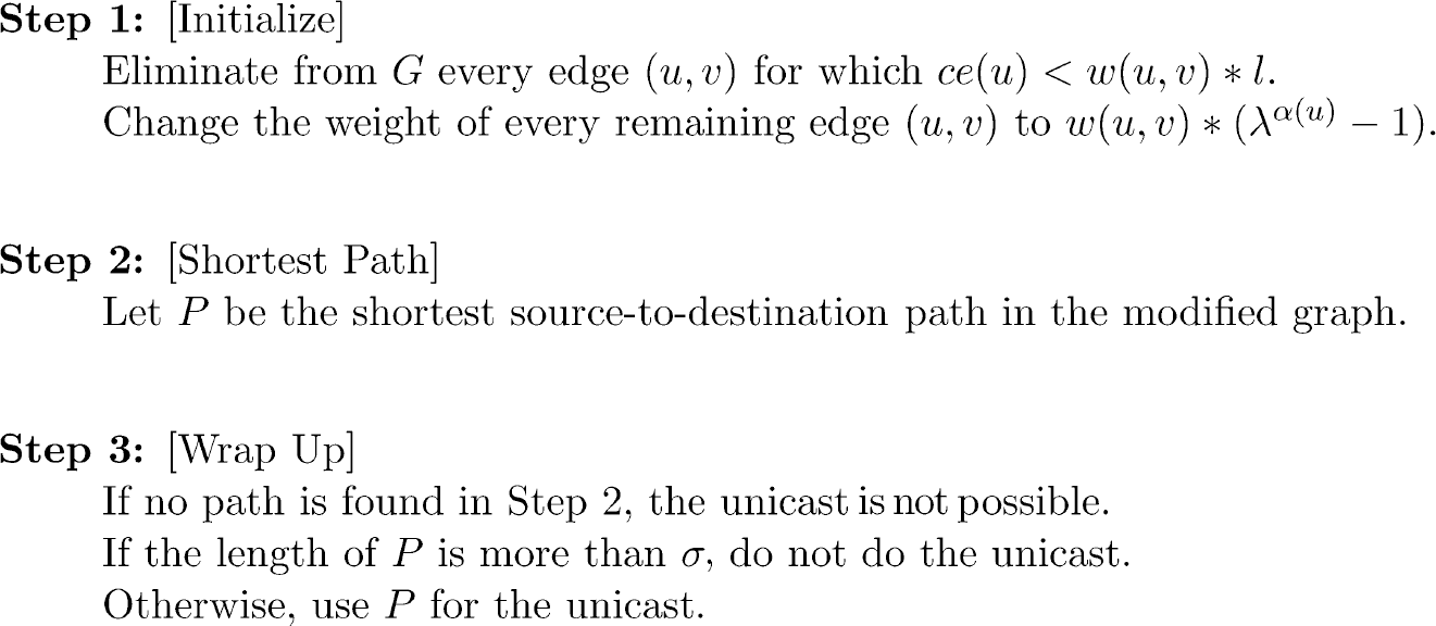
CMAX algorithm of [26] for unicasts.

The CMAX algorithm of Fig. 7 has a complexity advantage over the max–min zP_min algorithm of Fig. 6. The former does only one shortest-path computation per unicast, while the latter does O(logn), where n is the number of sensor nodes. Although admission control is necessary to establish the logarithmic competitive-ratio bound for CMAX, we may use CMAX without admission control (i.e., route every unicast that is feasible) by setting σ = ∞. Experimental results reported in [26] suggest that CMAX with no admission control outperforms max–min zP_min on both the lifetime and capacity metrics.

In the MRPC lifetime-maximization algorithm of Misra and Banerjee [36], the capacity, c(u, v) of edge (u, v) is defined to be ce(u)/w(u, v). Note that c(u, v) is the number of unit-length messages that may be transmitted along (u, v) before node u runs out of energy. The lifetime of path P, life(P) is defined to be the minimum edge capacity on the path. In MRPC, the unicast is done along a path P with maximum lifetime. Figure 8 gives the MRPC unicast algorithm. A decentralized implementation as well as a conditional MRPC in which minimum-energy routing is used so long as the selected path has a lifetime that is greater than or equal to a specified threshold. When the lifetime of the selected path falls below this threshold, we switch to MRPC routing.

Figure 8

MRPC algorithm of [36] for unicasts.

Chang and Tassiulas [6], [7] developed a linear-programming formulation for lifetime maximization. This formulation requires knowledge of the rate at which each node generates unicast messages. Wu, Gao, and Stojmenovic [53] proposed unicast routing based on connected dominating sets to maximize network lifetimes. Stojmenovic and Lin [44] and Melodia et al. [35] developed localized unicast algorithms to maximize lifetime, and Heinzelman, Chandrakasan, and Balakrishnan [16] developed a clustering-based routing algorithm (LEACH) for sensor networks.

3.2 Multicast and Broadcast

Using an omnidirectional antenna, node i can transmit the same unit message to nodes j₁, j₂, …, j_k, using

e_{w i r e l e s s} = max {w (i, j_{q}) ∣ 1 \leq q \leq k}

energy rather than

e_{w i r e d} = \sum_{q = 1}^{k} w (i, j_{q})

energy. Because c_wireless ≤ e_wired, the reduction in energy needed to broadcast from one node to several others in a wireless network over that needed in a wired network is referred to as the wireless broadcast advantage [50], [51].

Because of the similarity between multicast and broadcast algorithms for wireless sensor networks, we need to focus on just one of multicast and broadcast. In this paper, our explicit focus is broadcast. To broadcast from a source s, we use a broadcast tree T, which is a spanning tree of G that is rooted at s. The energy, e(u), required by a node of T to broadcast to its children is

e (u) = max {w (u, v) ∣ v is a child of u}

Note that for a leaf node u, e(u) = 0. The energy, e(T), required by the broadcast tree to broadcast a unit message from the source to all other nodes is

e (T) = \sum_{u} e (u)

For simplicity, we assume that only unit-length messages are broadcast. So, following a broadcast using the broadcast tree T, the residual energy, re(i, T), at node i is

r e (i, T) = c e (i) - max {w (i, j) ∣ j is a child of i in T} \geq 0

The problem, MEBT, of finding a minimum-energy broadcast tree rooted at a node s is NP-hard, because MEBT is a generalization of the connected dominating set problem, which is known to be NP-hard [14]. In fact, MEBT cannot be approximated in polynomial time within a factor (1 − ∊)Δ, where ∊ is any small positive constant, and Δ is the maximal degree of a vertex, unless NP ⊆ DTIME[n^O(loglogn)] [15]. Marks et al. [31] proposed a genetic algorithm for MEBT, and Das et al. [9] proposed integer programming formulations.

Wieselthier et al. [50], [51] proposed four centralized greedy heuristics—DSA, MST, BIP, BIPPN—to construct minimum-energy broadcast trees. The DSA (Dijkstra's shortest-path algorithm) heuristic (this is the BLU of [50], [51] augmented with the sweep pass of [50], [51]) constructs a shortest path from the source node s to every other vertex in G. The constructed shortest paths are superimposed to obtain a tree T rooted at s. Finally, a sweep is performed over the nodes of T. In this sweep, nodes are examined in ascending order of their index (i.e., in the order 1, 2, 3, …, n). The transmission energy τ(i) for node i is determined to be

max {w (i, j) ∣ j is a child of i in T}

If using τ(i) energy, node i is able to reach any descendents other than its children, then these descendents are promoted in the broadcast tree T and become additional children of i.

The MST (minimum spanning tree) (this is the BLiMST heuristic of [50] augmented with a sweep pass) uses Prim's algorithm [40] to construct a minimum-cost spanning tree (the cost of a spanning tree is the sum of its edge weights). The constructed spanning tree is restructed by performing a sweep over the nodes to reduce the total energy required by the tree.

The BIP (broadcast incremental power) heuristic (this is the BIP heuristic of [50], [51] augmented with a sweep pass) begins with a tree T that comprises only the source node s. The remaining nodes are added to T one node at a time. The next node u to add to T is selected so that u is a neighbor of a node in T, and e(T ∪ {u})–e(T) is minimum. Once the broadcast tree is constructed, a sweep is done to restructure the tree so as to reduce the required energy.

The BIPPN (broadcast incremental power per node) heuristic (this is the node-based MST heuristic of [51] augmented with a sweep pass) begins with a tree T that comprises only the source node s and uses several rounds to grow T into a broadcast tree. To describe the growth procedure, we define e(T, v, i), where v ∊ T, to be the minimum incremental energy (i.e., energy above the level at which v must broadcast to reach its present children in T) needed by node v so as to reach i of its neighbors that are not in T [of course, only neighbors j such that ce(v) ≥ w(v, j) are to be considered]. Let R(T, v, i) = i/e(T, v, i). Note that R(T, v, i) is the inverse of the incremental energy needed per node added to T. In each round of BIPPN, we determine v and i such that R(T, v, i) is maximum. Then, to T, we add the i neighbors of v that are not in T and can be reached from v by incrementing v's broadcast energy by e(T, v, i). The i neighbors are added to T as children of v. Once the broadcast tree is constructed, a sweep is done to restructure the tree so as to reduce the required energy.

Wan et al. [48] showed that when w(i, j) = c∗r^d, the MST and BIP heuristics have constant approximation ratios, and that the approximation ratio for DSA is at least n/2. Park and Sahni [37] described two additional centralized greedy heuristics—maximum energy node (MEN) and broadcast incremental power with look ahead (BIPWLA)—to construct minimum-energy broadcast trees. The second of these (BIPWLA) is an adaptation of the modified greedy algorithm proposed by Guha and Khuller [15] for the connected dominating set problem.

The MEN heuristic attempts to use nodes that have more energy as non-leaf nodes of the broadcast tree [note that when i is a nonleaf, re(i) < ce(i), whereas when i is a leaf, re(i) = ce(i)). In MEN, we start with T = {s}. At each step, we determine Q such that

Q = {u ∣ u is a leaf of T and u has a neighbor j, j \notin T, for which w (u, j) \leq c e (u)}

(1)

From Q, we select the node u that has maximum energy ce(u). All neighbors j of u not already in T and that satisfy w(u, j) ≤ ce(u) are added to T as children of u. This process of adding nodes to T terminates when T contains all nodes of G (i.e., when T is a broadcast tree). Finally, a sweep is done to restructure the tree so as to reduce the required energy.

The BIPWLA heuristic is an adaptation of the look-ahead heuristic proposed in [15] for the connected dominating set problem. This heuristic may also be viewed as an adaptation of BIPPN. In BIPWLA, we begin with a tree T that comprises the source node s together with all neighbors of s that are reachable from s using ce(s) energy. Initially, the source node s is colored black; all other nodes in T are gray, and nodes not in T are white. Nodes not in T are added to T in rounds. In a round, one gray node will have its color changed to black, and one or more white nodes will be added to T as gray nodes. It will always be the case that a node is gray iff it is a leaf of T; it is black iff it is in T but not a leaf; it is white iff it is not in T. In each round, we select one of the gray nodes g in T; color g black; and add to T all white neighbors of g that can be reached using ce(g) energy. The selection of g is done in the following manner. For each gray node u ∊ T, let n_u be the number of white neighbors of u reachable from u by a broadcast the uses ce(u) energy. Let p_u be the minimum energy needed to reach these n_u nodes by a broadcast from u. Let,

A (u) = {j ∣ w (u, j) \leq c e (u) and j is a white node}

We see that n_u = |A(u)|, and p_u = max{w(u, j)| j ∊ A(u)}.

For each j ∊ A(u), we define the following analogous quantities:

\begin{aligned} B (j) = {q ∣ w (j, q) \leq c e (j) and q is a while node} \\ n_{j} = | B (j) | \\ p_{j} = max {w {j, q} ∣ q \in B (j)} \end{aligned}

Node g is selected to be the gray node u of T that maximizes

n_{u} / p_{u} + max {n_{j} / p_{j} ∣ j \in B (u)}

Once the broadcast tree is constructed, a sweep is done to restructure the tree so as to reduce the required energy.

A localized distributed heuristic for MEBT that is based on relative neighborhood graphs has been proposed by Cartigny, Simplot, and Stojmenovic [4]. Wu and Dai [52] developed an alternative localized distributed heuristic that uses k-hop neighborhood information.

In a real application, the wireless network will be required to perform a sequence B = b₁, b₂, …, b_i; of broadcasts. Broadcast b_i will specify a source node s_i and a message length l_i. Assume, for simplicity, that l_i = 1 for all i. For a given broadcast sequence B, the network lifetime is the largest i such that broadcasts b₁, b₂, …, b_i are successfully completed. The six heuristics of [50], [51], [37] may be used to maximize lifetime by performing each b_i using the broadcast tree generated by the heuristic. (The broadcast trees are generated in sequence using the residual node energies.) However, because each of these heuristics is designed to minimize total energy consumed by a single broadcast, it is entirely possible that the very first broadcast depletes the energy in a node, making subsequent broadcasts impossible.

Singh, Raghavendra, and Stepanek [41] proposed a greedy heuristic for a broadcast sequence. The source node broadcasts to each of its neighbors resulting in a two-level tree T with the source as root. T is expanded into a broadcast tree through a series of steps. In each step, a leaf of T is selected, and its nontree network neighbors are added to T. The leaf selection is done using a greedy strategy—select the leaf for which the ratio (energy expended by this leaf so far)/(number of nontree leaves) is minimum.

The critical energy, CE(T), following a broadcast that uses the broadcast tree T is defined to be

C E (T) = min {r e (i, T) ∣ 1 \leq i \leq n}

Park and Sahni [37] suggested the use of broadcast trees that maximize the critical energy following each broadcast. Let MCE(G, s) be the maximum critical energy following a broadcast from node s. For each node i of G, define a(i) as below:

a (i) = {c e (i) - w (i, j) ∣ (i, j) is an edge of G and c e (i) \geq w (i, j)}

Let l(i) denote the set of all possible values for re(i) following the broadcast. We see that

l (i) = {\begin{cases} a (i) & if i = s \\ a (i) \cup {c e (i)} & otherwise \end{cases}

Consequently, the sorted list of all possible values for MCE(G, s) is given by

L = s o r t (\cup_{1 \leq i \leq n} l (i))

We may determine whether G has a broadcast tree rooted at s such that CE(T) ≥ q by performing either a breadth-first or depth-first search [40] starting at vertex s. This search is forbidden from using edges (i, j) for which ce(i) – w(i, j) < q. MCE(G, s) may be determined by performing a binary search over the values in L [37].

Each of the heuristics described in [50], [51], [37] to construct a minimum-energy broadcast tree may be modified so as to construct a minimum-energy broadcast tree T for which CE(T) = MCE(G, s). For this modification, we first compute MCE(G, s) and then run a pruned version of the desired heuristic. In this pruned version, the use of edges for which ce(i) - w(i, j) < MCE(G, s) is forbidden. Experiments reported in [37] indicate that this modification significantly improves network lifetime, regardless of which of the six base heuristics is used. Lifetime improved, on average, by a low of 48.3% for the MEN heuristic to a high of 328.9% for the BIPPN heuristic. The BIPPN heuristic modified to use MCE(G, s), as above, results in the best lifetime.

3.3 Data Collection and Distribution

In the data collection problem, a base station is to collect sensed data from all deployed sensors. The data distribution problem is the inverse problem, in which the base station has to send data to the deployed sensors (different sensors receive different data from the base station). In both of these problems, the objective is to complete the task in the smallest amount of time. Florens and McEliece [11], [12] have observed that the data collection and distribution problems are symmetric. Hence, one can derive an optimal data collection algorithm from an optimal data distribution algorithm and vice versa. Therefore, it is necessary to study just one of these two problems explicitly. In keeping with [11], [12], we focus on data distribution.

Let S₁, …, S_n be n sensors, and let S₀ represent the base station. Let p_i be the number of data packets the base station has to send to sensor i, 1 ≤ i ≤ n. p = [p₁, p₂, …, p_n]is the transmission vector. We assume that the distribution of these packets to the sensors is done in a synchronous time-slotted fashion. In each time slot, an s_i may either receive or transmit (but not both) a packet. To facilitate the transmission of the packets, each S_i has an antenna with a range of r. In the unidirectional antenna model, S_i receives a packet only if that packet is sent in its direction from an antenna located, at most, r away. Because of interference, a transmission from S_i to S_j is successful iff the following are true:

j is in range, that is, d(i, j) ≤ r, where d(i, j) is the distance between S_i and S_j.

j is not, itself, transmitting in this time slot.

There is no interference from other transmissions in the direction of j. Formally, every S_k, k ≠ i, that is transmitting in this time slot in the direction of S_j is out of range. Here, out of range means d(k, j) ≥ (1 + δ)r, where δ > 0 is an interference constant.

In the omnidirectional antenna model, a packet transmitted by an Si is received by all S_j (regardless of direction) that are in the antenna's range. The constraints on successful transmission are the same as those for the unidirectional antenna model, except that all references to “direction” are dropped. Our objective is to develop an algorithm to complete the specified data distribution using the fewest number of time slots. A related data-gathering problem for wireless sensor networks is considered in [59].

3.3.1 Unidirectional Antenna Model

Florens and McEliece [11] developed an efficient algorithm to distribute data in a tree network using the fewest number of time slots. This algorithm is an extension of their data-distribution algorithm for a line network. We look only at the details of the line-network algorithm here. In a line network, S₀, …, S_n are uniformly spaced on a straight line as in Fig. 9. The base station, S₀, is at the left end of the line, and the spacing is g. We assume that (1 + δ)r/2 ≤ g ≤ r. Hence, when S_i transmits a packet to its right, the packet can be received by S_i+1 but not by S_i+2.

Figure 9

A three-sensor line network; S₀ is the base station.

Consider the transmission vector [2, 0, 0] that requires two packets to be sent to S₁ and zero to the remaining sensors. This transmission may be completed in two time slots. S₀ sends a packet in each of these two time slots to S₁. The transmission vector [0, 2, 0] requires four time slots. In the first, S₀ sends the first packet to S₁. In the second time slot, only one of S₀ and S₁ may transmit, as if both transmit, then S₁ will need to receive (from S₀) and send (to S₁) in the second time slot. This violates the restriction that a sensor cannot receive and send in the same time slot. To avoid buffering problems at a sensor, we adopt a transmission discipline in which a packet is routed in consecutive slots until it reaches its destination. Adhering to this discipline requires that S₁ transmit, in slot 2, the packet it received in slot 1. So, in slot 2, the base station S₀ is idle. The remaining packet that is to be sent to S₂ is sent in slots 3 and 4. Notice that [2, 0, 1] can be done in four slots—in slot 1, S₀ sends to S₁; in slot 2, S₁ sends to S₂; in slot 3, S₀ sends to S₁ and S₂ sends to S₃; and in slot 4, S₀ sends to S₁.

With the no-buffering discipline, it is only the base station that has to make a decision for each time slot. If a sensor receives a packet that is destined for a sensor further down the line, it simply retransmits this packet in the next time slot. From our simple examples, it follows that the base station can transmit a packet in slot i + 1 iff it either did not transmit a packet in slot i, or the packet transmitted in slot i was destined for S₁. This feasibility constraint coupled with the greedy strategy to transmit packets in nonincreasing order of destination distance results in the greedy base-station algorithm of Florens and McEliece [11] (Fig. 10).

Figure 10

Base station algorithm of [11] for unidirectional antennas.

Let L(p) be the last slot in which any of the S_is transmits a packet when the base-station algorithm of Fig. 10 is used. Florens and McEliece [11], [13] have shown that

L (p) =_{l \leq i \leq n}^{max} {i - 1 + P_{i} + 2 \sum_{i + 1 \leq j \leq n} p_{j}}

and that this is the smallest possible value for L(p) over all feasible packet distribution strategies. Hence, the greedy algorithm of Fig. 10 is an optimal distribution algorithm. The optimality of the greedy algorithm holds even if sensors are permitted to buffer packets destined for other sensors.

Notice that the transmission schedule for the data distribution task defined by p may be converted into a data collection schedule with the same L(p) value. (For the data collection problem, p_i is the number of packets that the base station is to collect from the base station from S_i.) As noted in [11], each data distribution transmission from S_i to S_i+1 in time slot j becomes a data collection transmission from S_i+1 in time slot j becomes a data collection transmission from S_i+1 to S_i in time slot L(p)+1 – j.

3.3.2 Omnidirectional Antenna Model

The greedy unidirectional-antenna line-network algorithm of Fig. 10 may be modified to obtain an optimal distribution algorithm for a line network that employs omnidirectional antennas (Florens and McEliece [12]). This modified line-network algorithm may then be extended to obtain an optimal distribution algorithm for trees [12]. Florens and McEliece [12] also proposed a distribution algorithm for general networks. This distribution algorithm is within a factor 3 of optimal.

As we did for the unidirectional antenna model, we consider only the case of line networks here. Consider the line network of Fig. 9. We make the same assumptions as we did for the unidirectional model—synchronous time-slotted transmissions, a sensor cannot transmit and receive a packet in the same slot, and sensors do not buffer packets destined for other sensors. The unidirectional-antenna distribution strategy for p = [2, 0] and p = [0, 2] may be used for the omnidirectional-antenna case as well. However, the unidirectional strategy for p = [2, 0, 1] fails when applied to the case of omnidirectional antennas because of interference. In slot 3 of the unidirectional strategy, both S₀ and S₂ transmit a packet. Because S₁ is within range of both S₀ and S₂ (when omnidirectional antennas are used), the interference at S₁ causes the transmission from S₀ to S₁ to fail. In fact, every successful distribution strategy for [2, 0, 1] must use at least five slots when the S_i employ omnidirectional antennas. A possible five-slot distribution strategy is to use the first three slots to send S₃'s packet (from S₀ to S₁ to S₂ to S₃) and then use slots 4 and 5 to send the two packets for S₁.

With the no-buffering constraint, each sensor is required to forward, in the next slot, each packet it receives that is destined for another sensor. Only the base station has flexibility in operation. So, we need only develop a base-station algorithm that determines the slot in which each packet (regardless of its destination) is transmitted to S₁. Because of the omnidirectional interference properties, we see that packets destined for S₁ may be transmitted in successive slots; those destined for S₂ may be transmitted in alternate slots; and those destined for S_i, i > 2 may be transmitted only in every third slot. Coupling this observation with the greedy strategy of transmitting packets in nonincreasing order of destination distance results in the greedy algorithm of Fig. 11 [12]. The optimality of this algorithm is established in [12].

Figure 11

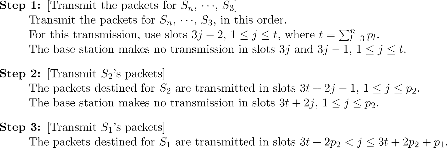
Base-station algorithm of [12] for omnidirectional antennas.

4. Sensor Fusion

The reliability of a sensor system is enhanced through the use of redundancy. That is, each point or region is monitored by multiple sensors. In a redundant sensor system, we are faced with the problem of fusing or combining the data reported by each of the sensors monitoring a specified point or region. Suppose that k > 1 sensors monitor point p. Let m_i, 1 ≤ i ≤ k be the measurement recorded by sensor i for point p. These k measurements may differ because of inherent differences in the k sensors, the relative location of a sensor with respect to p, as well as because one or more sensors is faulty. Let V be the real value for p. The objective of sensor fusion is to take the k measurements, some of which may be faulty, and determine either the correct measurement V or a range in which the correct measurement lies.

The sensor fusion problem is closely related to the Byzantine agreement problem that has been extensively studied in the distributed computing literature [27], [10]. Brooks and Iyengar [2] have proposed a hybrid distributed sensor-fusion algorithm that is a combination of the optimal region algorithm of Marzullo [32] and the fast convergence algorithm proposed by Mahaney and Schneider [30] for the inexact agreement version of the Byzantine generals problem. Let δ_i be the accuracy of sensor i. So, as far as sensor i is concerned, the real value at p is m_i ± δ_i (i.e., the value is in the range [m_i – δ_i, m_i + δ_i]). Each sensor needs to compute a range in which the true value lies as well as the expected true value. For this computation, each sensor sends its m_i and δ_i values to every other sensor. Suppose that sensor i is nonfaulty. Then, every nonfaulty processor receives the correct values of m_i and δ_i. Faulty sensors may receive incorrect values. Similarly, if processor i is faulty, the remaining processors may receive differing values of m_i and δ_i. Figure 12 gives the Brooks–Iyengar hybrid algorithm [2]. This algorithm is executed by every sensor using as data the measurement ranges received from the remaining sensors monitoring point p plus the sensor's own measurement.

Figure 12

Brooks–Iyengar hybrid algorithm to estimate V and range for V.

As an example computation, suppose that four sensors S1, S2, S3, and S4 monitor p, and that the four measurement ranges are [2], [6], [3], [8], [4], [10], and [1], [7]. To perform the computation specified by the Brooks–Iyengar hybrid algorithm, the four sensors communicate their measurement ranges to one another. Assume that S4 is the only faulty sensor. So, sensors S1, S2, and S3 correctly communicate their measurements to one another. However, these sensors may receive differing readings from S4. Likewise, S4 may record different receptions from S1, S2, and S3. Let the S4 measurement received by S1, S2, and S3 be [1], [3], [2], [7], [7], [12], respectively. The V and range computed at each of the four sensors are given in Fig. 13. Note that k = 4, and τ = 1.

Figure 13

Example for Brooks–Iyengar hybrid algorithm.

5. Conclusion

We reviewed some of the recent advances made in the development of algorithms for wireless sensor networks. This paper has focused on sensor deployment and coverage, routing (specifically, unicast and broadcast), and sensor fusion. Both centralized and distributed localized algorithms have been considered.

References

Aslam

, and Rus

, “Three power-aware routing algorithms for sensor network,” Wireless Communications and Mobile Computing 3, 187–208 (2003).

Brooks

and Iyengar

, “Robust distributed computing and sensing algorithm,” IEEE Computer, June, 53–60 (1996).

Cardei

and Du

, “Improving wireless sensor network lifetime through power aware organization,” ACM Wireless Networks, to appear.

Cartigny

Simplot

, and Stojmenovic

, “Localized minimum-energy broadcasting in ad-hoc networks,” IEEE INFOCOM (2003).

Chakrabarty

Iyengar

, and Cho

, “Grid coverage for surveillance and target location in distributed sensor networks,” IEEE Transactions on Computers, 51, 1448–1453, 2002.

Chang

and Tassiulas

, “Routing for maximum system lifetime in wireless ad-hoc networks,” 37th Annual Allerton Conference on Communication, Control, and Computing, Monticello, IL, September (1999).

Chang

and Tassiluas

, “Energy conserving routing in wireless ad-hoc networks,” IEEE INFOCOM (2000).

Culler

and Hong

, “Wireless sensor networks,” Special Issue, CACM 47(6) Singh (2004).

Das

A.K.

Marks

R.J.

, and El-Sharkawi

, “Minimum power broadcast trees for wireless networks,” IEEE International Symposium on Circuits and Systems, May (2002).

10.

Dolev

, “The Byzantine generals strike again,” J. of Algorithms. 14–30 (1982).

11.

Florens

and McEliece

, “Scheduling algorithms for wireless ad-hoc sensor networks,” IEEE GLOBECOM (2002), pp. 6–10.

12.

Florens

and McEliece

, “Packets distribution algorithms for sensor networks,” INFOCOM (2003).

13.

Florens

Francesdhetti

, and McEliece

, “Lower bounds on data collection time in sensory networks,” IEEE J. on Selected Areas in Communications 1 (11) (2004).

14.

Garey

and Johnson

, Computers and intractibility: A guide to the theory of NP-completeness, W. H. Freeman and Co., 1979.

15.

Guha

and Khuller

, “Approximation algorithms for connected dominating sets,” Fourth Annual European Symposium on Algorithms (1996).

16.

Heinzelman

Chandrakasan

, and Balakrishnan

, “Energy-efficient communication protocol for wireless microsensor networks,” IEEE HICSS (2000)

17.

Howard

Mataric

, and Sukhatme

, “An incremental self-deployment algorithm for mobile sensor networks,” Autonomous Robots, Special Issue on Intelligent Embedded Systems, 13, 113–126, 2002.

18.

Howard

Mataric

, and Sukhatme

, “Mobile sensor network deployment using potential fields: A distributed, scalable solution to the area coverage problem,” Sixth International Symposium on Distributed Autonomous Robotics Systems (DARS02) (2002).

19.

Huang

and Tseng

, “The coverage problem in a wireless sensor network,” WSNA (2003).

20.

Iyengar

and Brooks

, “Computing and communications in distributed sensor networks,” Special issue, J. of Parallel and Distributed Computing 64 (7) (2004).

21.

Iyengar

and Brooks

, Handbook of Distributed Sensor Networks (Chapman & Hall/CRC, Boca Raten, FL, 2005).

22.

Kannan

Sarangi

Iyengar

S. S.

, and Ray

, “Sensor-centric quality of routing in sensor networks,” INFOCOM (2003).

23.

Kannan

Sarangi

Ray

, and Iyengar

, “Minimal sensor integrity: Computing the vulnerability of sensor grids,” Info. Proc. Letters 86 (1), 49–55 (2003).

24.

Kannan

and Iyengar

S. S.

, “Game-theoretic models for reliable, path-length and energy-constrained routing in wireless sensor networks,” IEEE Journal on Selected Areas in Communications (2004).

25.

Kar

and Banerjee

, “Node placement for connected coverage in sensor networks,” Proc. WiOpt 2003: Modeling and Optimization in Mobile, Ad Hoc and Wireless Networks (2003).

26.

Kar

Kodialam

Lakshman

, and Tassiulas

, “Routing for network capacity maximization in energy-constrained ad-hoc networks,” IEEE INFOCOM (2003).

27.

Lamport

Shostak

, and Pease

, “The Byzantine generals problem,” ACM Trans. Prog. Lang. Syst. July, 499–516 (1986).

28.

Wan

, and Frieder

, “Coverage in wireless ad-hoc sensor networks,” IEEE Transactions on Computers 52, 753–763 (2002).

29.

and Tatsuya

, “Coverage-aware self-scheduling in sensor networks,” IEEE Computer Communications Workshop (CCW 2003) (2003).

30.

Mahaney

and Schneider

, “Inexact agreement: Accuracy, precision, and graceful degradation,” Fourth ACM Symp. on Principles of Distr. Computing (1985), pp. 237–249.

31.

Marks

Das

El-Sharkawi

Arabshahi

, and Gray

, “Minimum power broadcast trees for wireless networks: Optimizing using the viability lemma,” IEEE ISCAS (2002).

32.

Marzullo

, “Tolerating failures of continuous-valued sensors,” ACM Trans, Computer Systems November, 284–304 1990.

33.

Meguerdichian

Koushanfar

Potkonjak

, and Srivastava

, “Coverage problems in wireless ad-hoc sensor networks,” IEEE InfoCom (2001).

34.

Meguerdichian

Koushanfar

, and Potkonjak

, “Exposure in wireless ad hoc sensor networks,” Seventh Annual International Conference on Mobile Computing and Networking (MobiCom'01) (2001), pp. 139–150.

35.

Melodia

Pompili

, and Akyildiz

, “Optimal local topology knowledge for energy efficient geographical routing in sensor networks,” IEEE INFOCOM (2004).

36.

Misra

and Banerjee

, “MRPC: Maximizing network lifetime for reliable routing in wireless,” IEEE Wireless Communications and Networking Conference (WCNC) (2002).

37.

Park

and Sahni

, “Maximum lifetime broadcasting in wireless networks,” submitted.

38.

Poduri

and Sukhatme

, “Constrained coverage for mobile sensor networks,” IEEE Intl. Conf. on Robotics and Automation (ICRA'04) (2004), pp. 165–171.

39.

Rappaport

, Wireless Communications: Principles and Practices (Prentice Hall, New York, 1996).

40.

Sahni

, Data Structures, Algorithms, and Applications in Java, 2nd ed. (Silicon Press, NJ, 2005).

41.

Singh

Raghavendra

, and Stepanek

, “Power-aware broadcasting in mobile ad hoc networks,” IEEE PIMRC'99, Osaka, Japan, September (1999).

42.

Singh

Woo

, and Raghavendra

, “Power-aware routing in mobile ad hoc networks,” ACM/IEEE MOBICOM (1998).

43.

Slijepcevic

and Potkonjak

, “Power efficient optimization of wireless sensor networks,” IEEE Intl. Conf. on Communications (2001).

44.

Stojmenovic

and Lin

, “Power-aware localized routing in wireless networks,” IEEE Transactions on Parallel and Distributed Systems, 12, 1122–1133, (2000).

45.

Szewezyk

Osterweil

Polastre

Hamilton

Mainwaring

, and Estrin

, “Habitat monitoring with sensor networks,” CACM, 47 (6), 34–40 (2004).

46.

Tian

and Georganas

, “A coverage-preserving node scheduling scheme for large wireless sensor networks.” WNSA 2002, Atlanta, Georgia, 2002.

47.

Veltri

Huang

, and Potkonjak

, “Minimal and maximal exposure path algorithms for wireless embedded sensor networks,” SenSys'03 (2003).

48.

Wan

Calinescu

, and Frieder

, “Minimum-energy broadcast routing in static ad hoc wireless networks,” IEEE INFOCOM (2001).

49.

Wang

, “Integrated coverage and connectivity configuration in wireless sensor networks,” SenSys (2003).

50.

Wieselthier

Nguyen

, and Ephremides

, “On the construction of energy-efficient broadcasting and multicast trees in wireless networks,” IEEE INFOCOM (2000).

51.

Wieselthier

and Nguyen

, “Algorithm for energy-efficient multicasting in static ad hoc wireless networks,” Mobile Networks and Applications 251–261 (2001).

52.

and Dai

, “Broadcasting in ad-hoc networks based on self pruning,” IEEE INFOCOM (2003).

53.

Gao

, and Strojmenovic

, “On calculating power-aware connected dominating sets for efficient routing in ad hoc wireless networks,” J. Communications and Networks 4 (1) (2002).

54.

and Sahni

, “Optimal deployment of wireless sensors on a grid.”

55.

Heidermann

, and Estrin

, “Geography-informed energy conservation for ad hoc routing,” MOBICOM (2001).

56.

Yan

, and Stankovic

, “Differentiated surveillance for sensor networks,” First International Conference on Embedded Networked Sensor Systems (2003), pp. 51–62.

57.

Zhong

, and Zhang

, “PEAS: A robust energy conserving protocol for long-lived sensor networks,” 23rd ICDCS (2003).

58.

Zhong

, and Zhang

, “Energy efficient robust sensing coverage in large sensor networks,” Technical Report, UCLA (2002).

59.

Krishnamachari

, and Prasanna

, “Energy-latency tradeoffs for data gathering in wireless sensor networks,” INFOCOM (2004).

60.

Zhang

and Hou

, “Maintaining sensing coverage and connectivity in large sensor networks,” Technical Report UIUC, UIUCDCS-R-2003-2351 (2003).

61.

Zou

and Chakrabarty

, “Sensor deployment and target localization in distributed sensor networks,” ACM Transactions on Embedded Computing Systems 3 (1), 61–91 (2004).

Algorithms for Wireless Sensor Networks

Abstract

Keywords

1. Introduction

2. Sensor Deployment and Coverage

Theorem 1

Theorem 2

2.1 Deterministic Deployment

2.1.1 Region Coverage

2.3 Deployment Quality

3.1 Unicast

Theorem 3

3.3.1 Unidirectional Antenna Model

References