Sage Journals: Discover world-class research

Abstract

Aiming at the problem of wireless sensor network node coverage optimization with obstacles in the monitoring area, based on the grey wolf optimizer algorithm, this paper proposes an improved grey wolf optimizer (IGWO) algorithm to improve the shortcomings of slow convergence, low search precision, and easy to fall into local optimum. Firstly, the nonlinear convergence factor is designed to balance the relationship between global search and local search. The elite strategy is introduced to protect the excellent individuals from being destroyed as the iteration proceeds. The original weighting strategy is improved, so that the leading wolf can guide the remaining grey wolves to prey in a more reasonable way. The design of the grey wolf’s boundary position strategy and the introduction of dynamic variation strategy enrich the population diversity and enhance the ability of the algorithm to jump out of local optimum. Then, the benchmark function is used to test the convergence performance of genetic algorithm, particle swarm optimization, grey wolf optimizer, and IGWO algorithm, which proves that the convergence performance of IGWO algorithm is better than the other three algorithms. Finally, the IGWO algorithm is applied to the deployment of wireless sensor networks with obstacles (rectangular obstacle, trapezoidal obstacle and triangular obstacles). Simulation results show that compared with GWO algorithm, IGWO algorithm can effectively improve the coverage of wireless sensor network nodes and obtain higher coverage rate with fewer nodes, thereby reducing the cost of deploying the network.

Keywords

Wireless sensor network coverage optimization improved grey wolf algorithm coverage

Introduction

Coverage optimization is a basic problem of wireless sensor networks (WSNs).¹ In WSN, the perceptual nodes are generally scattered randomly, resulting in extremely low coverage rate and even problems such as network disconnection. Therefore, many researchers have studied this and achieved rich results.^2–5 In general, there are two types of network coverage optimization methods. Firstly, the coverage optimization based on geometric methods. For example, the blind-zone centroid-based scheme (BCBS) proposed in Wang et al.⁶ is optimized by using the geometric relationship between nodes, although the BCBS strategy has high coverage and high robustness, it still cannot achieve 100% coverage. Abo-Zahhad et al.⁷ proposed a centralized immune-Voronoi deployment algorithm (CIVA) based on Voronoi diagram, which uses Voronoi diagram attributes to balance coverage and energy consumption, improves WSN coverage, and extends the lifetime of the network. CIVA has a low computational complexity, but it has a “premature” problem. Secondly, application of intelligent optimization algorithm to complete dynamic coverage optimization of node deployment. Compared with the complex geometric derivation of Voronoi diagram, the intelligent optimization algorithm has the advantages of easy implementation and strong adaptability and is widely used in node optimization deployment. For example, the genetic algorithm (GA) characterized by biological genetic evolution^8–10 and the particle swarm optimization (PSO) algorithm for the flocking foraging process.^11,12 Xu and Yao⁸ proposed a coverage method of WSN optimized by GA, but this kind of method has the problem of falling into the local optimum, and the convergence speed is slow. In Liang and Lin,⁹ an adaptive GA for mutation probability and crossover probability was proposed to solve the problem of slow convergence, although this algorithm has a faster convergence rate, it is prone to fall into the problem of local optimum. Cong¹¹ proposed a PSO algorithm to improve the effective position of computing nodes, this algorithm improved the coverage rate of WSNs to some extent, but it still has a “premature” problem.

Grey wolf optimizer (GWO) algorithm is a meta-heuristic search algorithm inspired by Grey Wolf in recent years.¹³ Kamboj et al.¹⁴ applied the GWO algorithm to solve low-carbon shop scheduling problems; the author verifies that the optimized result of GWO algorithm is best by comparison with other intelligent algorithms, but the algorithm has the disadvantage of falling into local optimum. In Kaveh and Zakian,¹⁵ an improved grey wolf optimizer (IGWO) algorithm with additional tunable parameters was proposed and applied to the truss structure design, which can get better optimization results. In Pan et al.,¹⁶ a new GWOFPA algorithm was proposed, which combines flower pollination algorithm (FPA) and GWO, the position update strategy of FPA improves the direction and speed of grey wolf movement; the author finally verifies the effectiveness of the strategy by testing the benchmark function, but the GWOFPA is more complicated than GWO and has a longer running time. Shieh et al.¹⁷ proposed an IGWO algorithm by enriching population diversity. Although the algorithm enhances the ability to jump out of local optimum, the search precision of the solutions is low, and the author only applies it to obstacle-free objects, but the presence of obstacles and static nodes in the actual deployment is not discussed.

Most researchers discussed the deployment of sensor nodes in a barrier-free monitoring environment. Aiming at the shortages of basic GWO with slow convergence speed, low search precision and easy to fall into local optimum,¹⁸ and the problems encountered with the deployment of WSN nodes in the real environment, this paper discusses the deployment of sensor network with geometric obstacles (rectangle, trapezoid, and triangles) and the presence of static and dynamic sensor nodes in the monitoring area and proposes an IGWO algorithm based on the GWO algorithm, to solve the problem of slow convergence speed of GWO algorithm and easy to fall into local optimum, it can significantly improve the coverage rate of WSN and save the network deployment cost to a certain extent. The contributions of this paper are mainly reflected in the following aspects.

A nonlinear convergence factor is designed to replace the original linear convergence factor. The nonlinear convergence factor changes faster in the early iteration, which is conductive to the global optimization search, and the later change is slower, which is conductive to the local optimization search. Thereby speeding up the convergence of the algorithm. The elite strategy is introduced so that the good individuals in the last iteration will not be lost as the iteration progresses.

This paper improves the original equal weighting strategy, so that it can update the weight according to the influence ratio of the leading wolf, which is more in line with the characteristics of the grey wolf predation.

When the grey wolf individual is not in the predation range, it is proposed to update the grey wolf position according to the proportion, so that it is near the position of the leading wolf and enriched the diversity of the population. A variation strategy is introduced to solve the problem that GWO algorithm falls into local optimum due to the decrease of population diversity.

The nonlinear convergence strategy and the elite strategy are utilized to improve the convergence speed of the algorithm, the role of dynamic weight strategy is to improve the precision of the solution, and grey wolf position strategy and mutation strategy are used to expand the diversity of the wolves and enhance the ability of the algorithm to jump out of local optimum.

Model description

Network coverage model

Assume that the sensor nodes in the WSNs are isomorphic, and the sensing radius and communication radius are R_p and R_c, respectively. To ensure the connectivity of the WSN, the communication radius of the node is set to be greater or equal to twice the perceived radius of the node. Suppose that the set of wireless sensor nodes is S = {s₁, s₂, s₃, … , s_n}, the two-dimensional coordinates of any one sensor node s_i in the set are indicated as (x_i, y_i), the set of monitoring nodes is M = {m₁, m₂, m₃, … , m_n}, and the coordinates of any monitoring point m_j in the monitoring area as (x_j, y_j), then the Euclidean distance between the two points is described as follows

d (s_{i}, m_{j}) = \sqrt{{(x_{i} - x_{j})}^{2} + {(y_{i} - y_{j})}^{2}}

(1)

The monitoring probability of the node s_i to the monitoring point m_j is described as follows

p_{cov} (s_{i}, m_{j}) = {\begin{array}{l} 1 if d (s_{i}, m_{j}) \leq R_{p} \\ 0 otherwise \end{array}

(2)

Then the joint sensing probability of all sensor nodes to point m_j is described as follows

C_{p} (s_{all}, m_{j}) = 1 - \prod_{i = 1}^{n} (1 - p_{cov} (s_{i}, m_{j}))

(3)

where s_all is all sensor nodes within the measurement range. Assume that the monitored area is a rectangle of L × W. For the convenience of calculation, the rectangle is divided into L × W grids of equal area, and the center point of the grid is the monitoring node m. The monitoring probability of all monitoring points can be calculated, and the summation is the coverage area. The coverage rate C_r can be expressed as follows

C_{r} = \frac{\sum_{x = 1}^{L} \sum_{y = 1}^{W} C_{p} (S_{all}, p_{(x - 1) \cdot L + y})}{L \times W}

(4)

Network connectivity model

The most basic self-organizing requirement of WSN is that the network must be connected. For ease of calculation, 2 R_p = R_c is assumed. Set N = {N₁, N₂, N₃ … , N_n} is the node in the sensor network. If the distance between N_i and N_j is no greater than R_p, then N_i and N_j are adjacent. Set the edge to 1, otherwise set to 0 and establish the undirected graph adjacency matrix M . According to the matrix power algorithm in Mesbahi and Egerstedt,¹⁹ the equation of the matrix S is as follows

S = M + M^{2} + M^{3} + \dots M^{n - 1}

(5)

where n is the number of sensor nodes. If there is an element of value 0 in S , then the WSNs are not connected. Otherwise, WSNs are connected. On the basis of WSNs connectivity, the minimum spanning tree is generated according to the algorithm in Zhou et al.²⁰

Standard GWO algorithm

The GWO is a heuristic algorithm proposed by Mirjalili et al.¹³ The algorithm evolved from the hierarchy of wolves and the process of predation; it has good search ability and convergence.

Social hierarchy

The wolves are divided into four levels, which can be expressed as α, β, δ, and ω from high to low. Among them, α, β, and δ indicate the grey wolves with top 3 fitness levels, which indicate the current optimal solution, suboptimal solution, and general solution, respectively, and the remaining grey wolves’ population ω indicates the candidate solutions. The rank of grey wolf is based on the fitness. The higher the fitness in this study denotes the higher social level. In Figure 1, the α layer wolf has the largest fitness and the highest social level, and the level of wolves from layer α to layer ω is getting lower and lower. The α layer wolf is responsible for leading the ω layer to surround the prey, and the β and δ layer wolves jointly assist the α layer wolf to issue the rounding command. The social level of each wolf is not fixed, it will be redistributed according to the value of the fitness.

Figure 1.

Grey wolf social hierarchy pyramid.

Round up hunting

In order to make the ω layer wolves move closer to the prey, the α, β, and δ layer wolves with higher social ranks issued a round-up hunting command to the ω layer wolves, so that the ω layer wolves approach the prey from all directions and update their position.

As shown in Figure 2, among the many grey wolves, α, β, and δ are closest to the prey, and the approximate positions of the prey are simulated by the positions of α, β, and δ. After multiple iterations, the simulation is more accurate. After the α wolf issued a killing command to the ω wolves, the ω wolves updated their position to reach the prey. Calculate the distance between the ω wolves and α, β, and δ.

Figure 2.

Grey Wolf location update.

The mathematical description is as follows

{\begin{matrix} {\vec{D}}_{a} = {\vec{C}}_{1} * {\vec{X}}_{a} (t) - {\vec{X}}_{w} (t) \\ {\vec{D}}_{β} = {\vec{C}}_{2} * {\vec{X}}_{b} (t) - {\vec{X}}_{w} (t) \\ {\vec{D}}_{δ} = {\vec{C}}_{3} * {\vec{X}}_{d} (t) - {\vec{X}}_{w} (t) \end{matrix}

(6)

{\begin{matrix} {\vec{C}}_{1} = 2 * \vec{r_{1}} \\ {\vec{C}}_{2} = 2 * \vec{r_{1}} \\ {\vec{C}}_{3} = 2 * \vec{r_{1}} \end{matrix}

(7)

where vector

{\vec{D}}_{α} indicate

indicates the distance between the α wolf and the ω wolves, vectors

{\vec{D}}_{β}

the distance between the β wolf and the ω wolves, and

{\vec{D}}_{δ}

the distance between the δ wolf and the ω wolves. Vector

{\vec{X}}_{α} (t)

is the position of the α wolf in the tth (current) iteration, vectors

{\vec{X}}_{β} (t)

is the position of the β wolf in the tth (current) iteration, and

{\vec{X}}_{δ} (t)

is the position of the δ wolf in the tth (current) iteration. Vector

{\vec{X}}_{ω} (t) indicate

s the position of the ω wolves in the tth iteration;

{\vec{C}}_{1} indicate

s the direction vector when ω wolves move toward α and affects the orientation of the ω wolves movement, vectors

{\vec{C}}_{2}

the direction vector when ω wolves move toward β and affects the orientation of the ω wolves movement, and

{\vec{C}}_{3}

the direction vector when ω wolves move toward δ and affects the orientation of the ω wolves movement.

{\vec{r}}_{1}

is random vector in [0,1] .

Omega (ω) wolves learn the distance from α, β, and δ, respectively, approaching with a certain step length and eventually reaching near the prey. The location update of the ω wolves is described as follows

{\begin{matrix} {\vec{X}}_{1} = {\vec{X}}_{a} - {\vec{A}}_{1} * {\vec{D}}_{a} \\ {\vec{X}}_{2} = {\vec{X}}_{b} - {\vec{A}}_{2} * {\vec{D}}_{b} \\ {\vec{X}}_{3} = {\vec{X}}_{d} - {\vec{A}}_{3} * {\vec{D}}_{d} \end{matrix}

(8)

{\begin{matrix} {\vec{A}}_{1} = 2 a * \vec{r_{2}} - a \\ {\vec{A}}_{2} = 2 a * \vec{r_{2}} - a \\ {\vec{A}}_{3} = 2 a * \vec{r_{2}} - a \end{matrix}

(9)

a = 2 - 2 (\frac{t}{t_{\max}})

(10)

\vec{X} (t + 1) = ({\vec{X}}_{1} + {\vec{X}}_{2} + {\vec{X}}_{3}) / 3

(11)

If the ω wolves only regards the α wolf as the prey, ${\vec{X}}_{1}$ is the position vector of its next generation; if the ω wolves only regards the β wolf as the prey, vector ${\vec{X}}_{2} is the position vector of its next generation$ ; and if the ω wolves only regards the δ wolf as the prey, ${\vec{X}}_{3} is the position vector of its next generation$ . t is the current number of iterations, t_max is the maximum number of iterations, a is the convergence factor, and a decreases linearly from 2 to 0 as the number of iterations increases. Vector ${\vec{A}}_{1}$ is the step size of ω wolves movement. When | ${\vec{A}}_{1}$ | > 1, the wolves will expand the search range, and the wolves will be relatively scattered, which is conducive to global optimization search. On the contrary, the wolves will narrow the encirclement, and the position is relatively concentrated, which is conducive to local optimization search, vectors ${\vec{A}}_{2}$ and ${\vec{A}}_{3}$ and so on. ${\vec{r}}_{2}$ is random vector in [0,1]. The position vector $\vec{X} (t + 1)$ of the next generation is set to the arithmetic mean of ${\vec{X}}_{1}, {\vec{X}}_{2,}$ and ${\vec{X}}_{3}$ .

The pseudo code of the GWO algorithm is expressed as follows

Algorithm 1: grey wolf optimizer

Input: grey wolf population vectors $\vec{W}$ , population size n;

Output: grey wolf ${\vec{X}}_{α}$ ;

1 for t = 1 tot_maxdo

2 Initialize/update, ${\vec{A}}_{1}$ , ${\vec{A}}_{2}, {\vec{A}}_{3}, {\vec{C}}_{1}, {\vec{C}}_{2}$ , and ${\vec{C}}_{3}$ ;

3 Calculate the fitness of $\vec{W}$ and sort it ;

4 The best grey wolf of $\vec{W}$ as ${\vec{X}}_{α}$ ;

5 The second best grey wolf of $\vec{W}$ as ${\vec{X}}_{β}$ ;

6 The third best grey wolf of $\vec{W}$ as ${\vec{X}}_{δ}$ ;

7 index ← 1;

8 while index < n-2 do

9Calculate ${\vec{D}}_{α} {\vec{, D}}_{β}$ , ${\vec{D}}_{δ}$ , ${\vec{X}}_{1}, {\vec{X}}_{2}, and {\vec{X}}_{3}$ ;

10 $\vec{X} (t + 1)$ ← ( ${\vec{X}}_{1} + {\vec{X}}_{2} + {\vec{X}}_{3}$ )/3;

11index ← index + 1;

12//update the position of ω

13 end

14 end

15 return ${\vec{X}}_{α}$ ;

Improved GWO algorithm

Nonlinear convergence factor strategy

The GWO algorithm proved to have better convergence performance than the PSO algorithm.¹³ However, because the convergence factor is linearly decremented from 2 to 0, the global search and the local search have the same proportion in the whole search process, failing to balance the global search and the local search. Therefore, a nonlinear convergence factor strategy is proposed. The mathematical description is as follows

a = 2 - 2 {\sqrt{1 - (\frac{t_{\max} - t}{t_{\max}})}}^{2}

(12)

In Figure 3, a is nonlinearly decreasing from 2 to 0. The value of a in the early iteration changes relatively quickly, which is conductive to global search. In the latter part of the iteration, the value of a changes relatively slowly, and the step-size of grey wolf movement is small, which is beneficial to local search. Therefore, the convergence speed of the algorithm is improved.

Figure 3.

Comparison of convergence factors.

Elite strategy

In GWO algorithm, the ω wolves slowly arrive near the prey with the iteration, and the superior individuals of the previous generation may be lost as the iteration progresses. Therefore, the elite strategy is introduced, replacing the three wolves with the smallest fitness in ω wolves with α, β, and δ in the next generation. It can be described as

{\begin{matrix} wol f_{1} = α \\ wol f_{2} = β \\ wol f_{3} = δ \end{matrix}

(13)

Among them, wolf₁, wolf₂, and wolf₃ indicate the three wolves with the least fitness. This strategy can save the superior individuals of the previous generation to the next generation, so that more grey wolves can search for prey near the position of the leading wolf, thus speeding up the convergence of the algorithm.

Dynamic weighting strategy

In GWO algorithm, the three leading wolves have equal impact on the ω wolves. In fact, α wolf indicates the best individual of the current iteration, so α wolf is closer to the prey than β wolf and δ wolf. Therefore, the α wolf has the greatest impact on hunting prey, β wolf is second, and δ wolf is the smallest. Therefore, Wen and Tie-Bin²¹ proposed a strategy of using the proportion of fitness of the three leading wolves for guidance; f_α corresponds to the fitnesss of α wolf, and f_β and f_δ correspond to β and δ, respectively. It can be described as

{\begin{matrix} w_{1} = f_{α} / (f_{α} + f_{β} + f_{δ}) \\ w_{2} = f_{β} / (f_{α} + f_{β} + f_{δ}) \\ w_{3} = f_{δ} / (f_{α} + f_{β} + f_{δ}) \end{matrix}

(14)

This w₁, w₂, andw₃ correspond to the guiding rates of α, β, and δ, respectively. Then, the next position of the ω wolves can be expressed as follows

\vec{X} (t + 1) = w_{1} * {\vec{X}}_{1} + w_{2} * {\vec{X}}_{2} + w_{3} * {\vec{X}}_{3}

(15)

If there are negative numbers in the three fitness levels, the strategy proposed in Wen and Tie-Bin²¹ is not suitable for this situation; therefore, another guiding rate strategy is proposed to meet the predation characteristics of grey wolves, as shown in the following equation (16)

{\begin{array}{l} f_{b} = - (| f_{α} | + | f_{β} | + | f_{δ} |) \\ d_{α} = f_{α} - f_{b} \\ d_{β} = f_{β} - f_{b} \\ d_{δ} = f_{δ} - f_{b} \\ d_{s} = d_{α} + d_{β} + d_{δ} \end{array}

(16)

Set a reference position f_b, corresponding to the minimum value, and the distance from f_α, f_β, and f_δ to f_b are d_α, d_β, and d_δ, respectively, and the sum of the distances of the three is d_s. The distance between f_α with a large fitnesss and the reference f_b is the largest, and the distance between the f_δ with the smallest fitnesss and f_b is the smallest. Then the next generation ω wolves’ location update strategy can be expressed as follows

{\begin{array}{l} w_{1} = d_{α} / d_{s} \\ w_{2} = d_{β} / d_{s} \\ w_{3} = d_{δ} / d_{s} \\ \vec{X} (t + 1) = w_{1} * {\vec{X}}_{1} + w_{2} * {\vec{X}}_{2} + w_{3} * {\vec{X}}_{3} \end{array}

(17)

As shown in the equation (17), it is known that w₁ > w₂ > w₃. This strategy is consistent with the fact that the effects of α, β, and δ wolves on ω are sequentially reduced. This is in line with the original intention of the algorithm design.

Dynamic variation strategy

The GWO algorithm showed good convergence at the beginning, but with the iteration, almost all the grey wolves are distributed among the same position in the later stage, which led to the decrease of wolf population diversity, and the algorithm is easy to fall into local optimum. For this reason, a variation strategy proposed in the Xu et al.²² is cited in this paper. Set the mutation probability pv = 0.5, then the strategy is described as follows

{\begin{matrix} variation & rand < p v * (t_{\max} - t) / t_{\max} \\ no variation & otherwise \end{matrix}

(18)

where (t_max–t)/t_max varies linearly from 1 to 0. At the beginning of the iteration, the dynamic mutation probability is large, which can promote global search. The mutation probability is reduced in the late iteration, which promotes local search and avoids falling into local optimum. As shown in the equation (18), when the variation requirement is met, the algorithm performs the mutation operation. It should be noted that if the value of fitness after the mutation is worse than before the mutation, it will not mutate. The mutation strategy is described as follows

{\begin{array}{l} d_{upper} = l_{upper} - α \\ d_{lower} = α - l_{lower} \\ ω = α + rand * d_{upper} if rand > 0.5 \\ ω = α - rand * d_{lower} otherwise \end{array}

(19)

Based on the position of α wolf, the distance between the upper limit l_upper and lower limit l_lower of the grey wolf’s range and α wolf was calculated as d_upper and d_lower, respectively, rand is a random number, if its value is greater than 0.5, then the position of ω wolves is the sum of position of α wolf and rand*d_upper. On the contrary, ω is the difference between α and rand*d_lower. The variation strategy expands the diversity of the population and enhances the ability of the algorithm to jump out of the local optimum.

Grey wolf boundary position strategy

After multiple iterations of the GWO algorithm, the location of the ω wolf may be outside the scope of the hunting prey; if this problem occurs, it is necessary to correct the position of the ω wolf in time. To this end, the position vectors of ${\vec{X}}_{1} {\vec{X}}_{2}, and {\vec{X}}_{3}$ are adjusted. For convenience of description, vector $\vec{X}$ denotes one of ${\vec{X}}_{1} {\vec{X}}_{2}, and {\vec{X}}_{3}$ . There are three types of location adjustment strategies.

If the position of grey wolf is below the lower limit of the wolves’ hunting range, the ω wolves’ coordinate is updated to l_lower, and if the grey wolf position exceeds the wolves’ hunting range upper limit, the ω wolves’ position coordinate is updated to l_upper, and the mathematical description is as follows

{\begin{matrix} \vec{X} = l_{lower} & if \vec{X} < l_{lower} \\ \vec{X} = l_{upper} & if \vec{X} > l_{upper} \end{matrix}

(20)

When the grey wolf position is out of range, Mirjalili et al.¹³ proposed a strategy to randomly update a position in the boundary to replace the coordinates of wolves. It can be described as follows

\vec{X} = l_{lower} + (l_{upper} - l_{lower}) * rand

(21)

Replace high-level grey wolves with grey wolves that are not in the range of hunting prey. If ${\vec{X}}_{1}$ is offside, it is replaced with α wolf, and ${\vec{X}}_{2}$ and ${\vec{X}}_{3}$ are replaced with β and δ, respectively.

The first scheme replaces the position of the grey wolf with the boundary value of the upper and lower limits. During the iterative process, more and more grey wolves will be at the upper and lower limits, resulting in weaker wolf population diversity. Although the second scheme expands the diversity of the wolf population, it fails to make the wolves approach the leading wolf, which is not in line with the original intention of the algorithm design. The third scheme directly leads to the decline of wolf diversity, which makes the algorithm fall into local optimum. To this end, a more effective location update strategy is proposed. Take ${\vec{X}}_{1}$ and α wolves ${\vec{X}}_{2} and β wolves, and {\vec{X}}_{3}$ $and δ$ wolves as examples. The mathematical description is as follows

{\begin{array}{l} r_{lower} = \frac{α - l_{lower}}{α - \vec{X_{1}}} if \vec{X_{1}} < l_{lower} \\ \vec{X_{1}} = l_{lower} + α * r_{lower} \\ r_{upper} = \frac{l_{upper} - α}{\vec{X_{1}} - α} if \vec{X_{1}} > l_{upper} \\ \vec{X_{1}} = α + r_{upper} * (\vec{X_{1}} - α) \end{array}

(22)

When ${\vec{X}}_{1}$ is less than the lower limit l_lower, r_lower indicates the ratio of the distance between α and ${\vec{X}}_{1}$ as well as the distance between α and l_lower, meanwhile, the position of ${\vec{X}}_{1}$ is updated to the sum of l_lower and a*r_lower. When ${\vec{X}}_{1}$ is greater than the upper limit l_upper, r_upper indicates the ratio of the distance between l_upper and α and the distance between ${\vec{X}}_{1}$ and α, and the position of ${\vec{X}}_{1}$ is updated to the sum of α and r_upper*( ${\vec{X}}_{1}$ −α).

When the grey wolf is not within the predation range, its position is updated proportionally according to the above equation. This strategy is more in line with the principle that ω wolves approach three leading wolves and can increase population diversity.

Improved grey wolf algorithm description

Set the maximum number of iterations and the upper and lower limits of the position of the wolves, and initialize the wolves’ position in the upper and lower limits.

Initial/update a, ${\vec{A}}_{1}$ , ${\vec{A}}_{2}, {\vec{A}}_{3}, {\vec{C}}_{1}, {\vec{C}}_{2},$ and ${\vec{C}}_{3}$ according to equations (7), (9), and (12).

Calculate the fitness of each grey wolf.

Select the three grey wolves with the highest fitness as α, β, and δ and the rest as ω.

Elite strategy processing according to equation (13).

Calculate the distance between ω wolves and β and δ according to equation (6).

Update the wolf position according to equations (8), (14), and (15).

The wolves are mutated according to equations (18) and (19), and the wolves are processed out of range according to equation (22).

Determine whether the algorithm meets the iteration stop condition, not meet then jump to step 2, otherwise output grey α wolf position, the end of the algorithm.

When the IGWO algorithm is applied to the WSN node coverage optimization deployment, the coverage rate is the evaluation index. After the iteration is completed, the connectivity of the nodes is determined according to equation (5). On the basis of connectivity, a deployment scheme (the grey wolf individual) with the largest coverage rate is selected as the final solution (Figure 4).

Figure 4.

IGWO algorithm flow chart.

Algorithm complexity analysis

Suppose m is the maximum number of iterations of the algorithm, n is the population size, and d is the dimension of the optimization problem. The GWO algorithm first initializes the population, and its time complexity is O(dn). Secondly, the fitness is calculated according to the position of the grey wolf, the time complexity is O(n). And then sorted in ascending order according to the value of the fitness. The time complexity is O(nlogn). Finally, the position of the grey wolf population is updated according to the above equation, and the time complexity is O(n), so the total time complexity is O(m(dn + n + nlogn + n)). Compared with the GWO algorithm, the IGWO algorithm adds mutation steps, and its time complexity is O(n), so the total time complexity of IGWO is O(m(dn + n + nlogn + n + n)). Comparing the two algorithms, when the value of n is very small, it is known that they belong to the same order of magnitude, and the time complexity is O(mnlogn).

Simulation experiments

In order to verify the performance of the IGWO algorithm, two experiments were performed. Experiment 1 used the test function to verify the convergence performance of the IGWO algorithm. Experiment 2 tested the precision of algorithm on the optimal deployment of the wireless sensor nodes. The experiment is carried out in Intel core i5 dual-core CPU, clocked at 2.4 GHz, memory 8GB, Windows 10 environment, experimental simulation software using matlab 2014 b.

Experiment 1—comparison of algorithm convergence

The F(x): maxf(x) = xsin(x)cos(2x)–2xsin(3x) test function is used to perform function optimization and convergence test. The F(x) search range is set to [0, 30], compared with GA,²³ PSO,²⁴ and original GWO. GA is a classic swarm intelligence algorithm, and PSO is famous for its remarkable effect in searching for optimal solutions and superior convergence performance. All comparison algorithms set 30 search agents uniformly. The number of algorithm iterations was set to 200 times and run 20 times. Finally, the average of 20 experimental results was obtained. To reduce the error, the mean is expressed as the average of the two extremes (maximum and minimum) removed.

Figure 5 depicts the test results of the four algorithms on the function F(x). It can be seen from the figure that the IGWO algorithm searches for the optimal solution after 21 iterations, while the GA, PSO, and GWO all take about 60 times, and the convergence speed of the IGWO algorithm has obvious advantages. On the one hand, because the elite strategy is introduced, the current optimal solution will not be destroyed by the iteration of the algorithm. Instead, the search solution can be continued from the vicinity of the current optimal solution, thus accelerating the convergence of the algorithm. On the other hand, because the nonlinear convergence factor is used in IGWO, the global optimization ability of the algorithm is enhanced, which effectively guides the grey wolf to approach the global optimal direction, thereby jumps out of the local optimum and speeding up the optimization. In the GA that evolves into genetic characteristics, the mutation strategy tends to destroy good individuals in the iterative process, and thus, the convergence is slower. The PSO evolved by bird flight according to the global optimal solution to the population and the individual local optimal solution dynamically updates the individual position, which makes it converge faster, but it is easy to fall into the local optimal state because of the decrease of population diversity of the later iteration. The linear convergence factor of the GWO algorithm does not weigh the time between the global optimization search and the local optimization search, and thus, the convergence is slower than IGWO. Compared with these three algorithms, the nonlinear convergence factor strategy is effective against the convergence of the IGWO algorithm. However, its performance on the running time is not excellent. The simulation time of GA, PSO, GWO, and IGWO is 0.042 s, 0.025 s, 0.029 s, and 0.033 s, respectively. GA has the longest running time because of its complicated procedures and relatively difficult to implement the details of the algorithm. PSO and GWO have fewer procedures, so the running time is shorter, and the IGWO algorithm has a slightly longer running time than the GWO algorithm due to the increased mutation operation.

Figure 5.

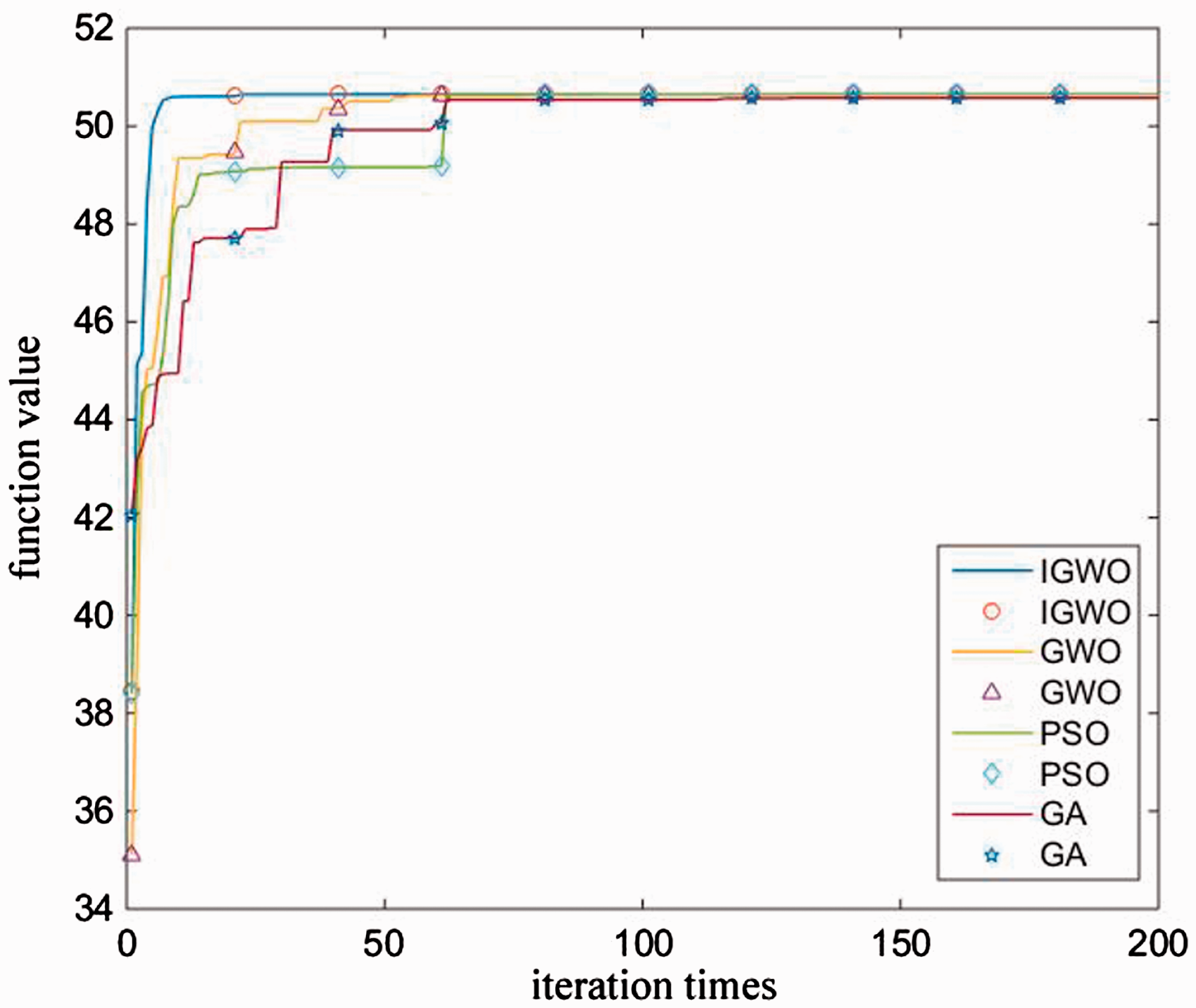
Algorithm test result.

Experiment 2—comparison of node coverage

This section tests the WSN node coverage optimization effect. Due to the complexity of the sensor network node deployment environment, four sets of experiments were designed, including the obstacle-free situation, the presence of rectangular obstacles, the presence of trapezoidal obstacles, and the coverage area being polygonal. In order to eliminate the error caused by randomness, 20 experiments were performed in each experimental scene, and the number of iterations was set 200 times for each experiment, and the final average results were compared. The monitoring area is 2500 m², 2300 m², 2050 m², and 2050 m², respectively. All sensor nodes are movable and isomorphic, setting the node’s perceived radius to 5 m and the communication radius to 10 m. When the node movement function fails, the node sensing radius is set to 7.5 m and the communication radius is 15 m. The specific parameter settings are shown in the Table 1.

Table 1.

Parameter settings.

Groups	Area size (m²)	Search agent (number)	Number of iterations	Number of nodes	Static node (number)	Obstacle shapes
1	2500	50	200	30,35,40,45,50,55	0	No
2	2300	50	200	20,25,30,35,40,45,50,55	2	Rectangle
3	2050	50	200	20,25,30,35,40,45,50,55	2	Trapezoid
4	2050	50	200	20,25,30,35,40,45,50,55,60	2	Triangle

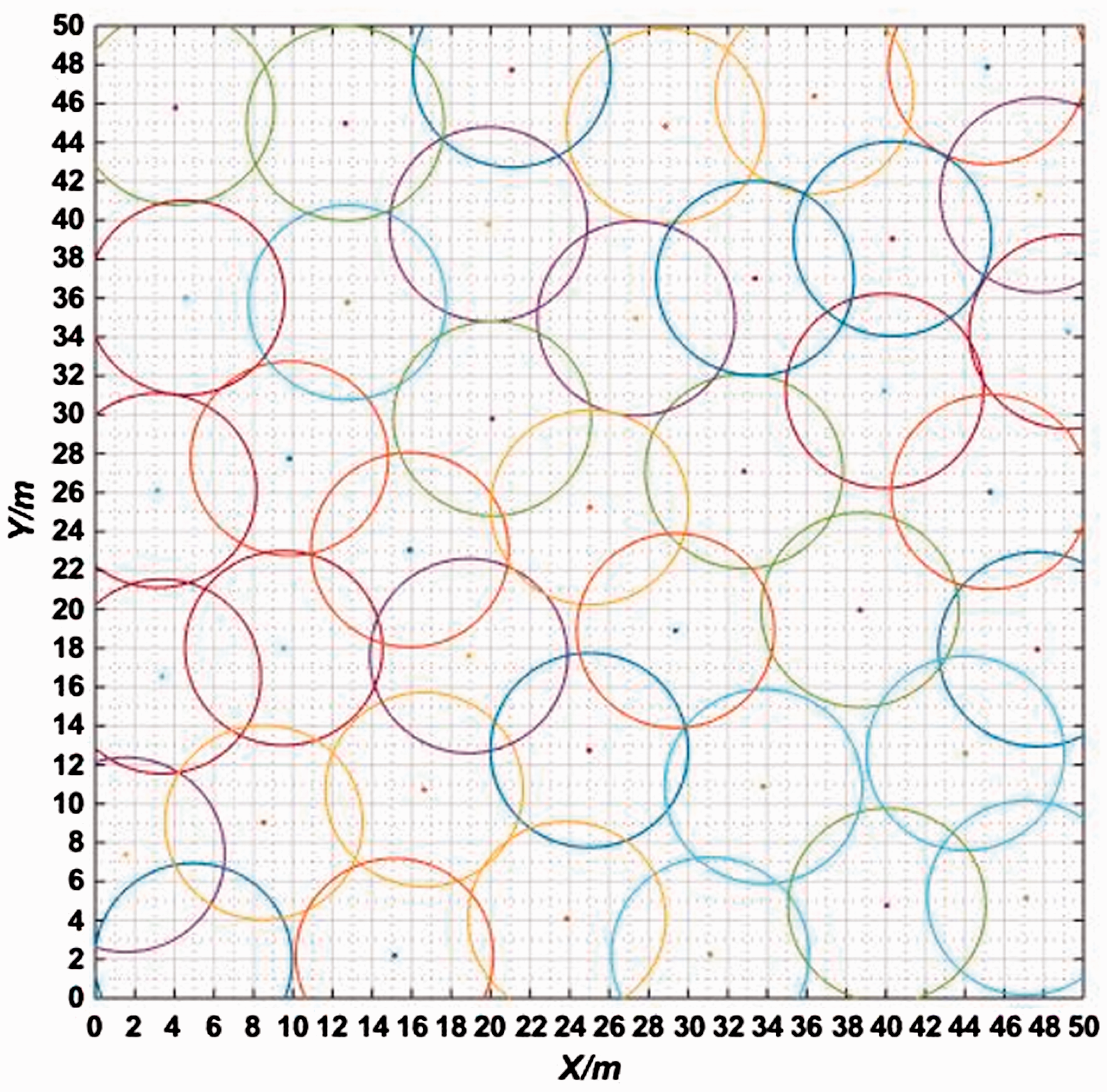
Figures 6 to 9 show the node deployment effect and algorithm coverage comparison for the case of no obstacles and no static sensor nodes. Figure 6 shows the coverage effect of nodes deployed in random mode. It can be seen that the nodes are not evenly distributed, some nodes even overlap, and the network is not connected. After the IGWO algorithm is used to optimize the node deployment location, as shown in Figure 7, the node location is relatively uniform. On the basis of ensuring the connectivity of the node, the coverage rate is greatly improved. Figure 8 describes the coverage comparison between the optimal deployment of GWO algorithm and the optimal deployment of IGWO algorithm when the number of sensor nodes is 40. It can be seen that IGWO algorithm enters the convergence stage when it is iterated for about 150 times, and the node coverage reaches about 97.5%, while GWO algorithm does not converge when it is iterated for 200 times, and it can be seen from the figure that the GWO algorithm has been fallen into the local optimum multiple times during the iterative process. This is because the grey wolf individual gathers near the prey in the later iteration, and the population diversity will be weakened, so that the search efficiency is reduced. The IGWO algorithm can maintain the diversity of the population to some extent due to the adaptive mutation strategy, and the ability to jump out of the local optimum is also enhanced. Figure 9 describes the coverage comparison of random, GWO, and IGWO algorithms under different number of nodes. It can be known that the coverage of GWO and IGWO algorithm is significantly higher than that of random algorithm under the premise of the same number of nodes. This is because the random algorithm is aimlessly looking for the target, which is very inefficient, and the intelligent optimization algorithm is heuristic to search, evaluate the function of each search position, get a current best position, and then searching from this location to the target is a purposeful and inspiring way to search for goals, which is more efficient. In the comparison between IGWO and GWO, 100% coverage rate can be achieved when the number of nodes is greater than 55, but when the number of nodes is less than 55, the coverage rate of IGWO algorithm is higher, because it updates the location with a more reasonable dynamic weighting strategy; first get the three best node deployment scheme (α wolf, β wolf, and δ wolf), and obtain the corresponding coverage rate, dynamically guide other node deployment schemes (ω wolves) to optimize according to the proportion of the three coverage rate. This strategy is more flexible and reasonable than GWO’s weighting strategy based on location averaging, so the network coverage rate of IGWO algorithm deployment is higher.

Figure 6.

Initial deployment.

Figure 7.

IGWO optimized deployment.

Figure 8.

Coverage rate.

Figure 9.

Number and coverage of nodes.

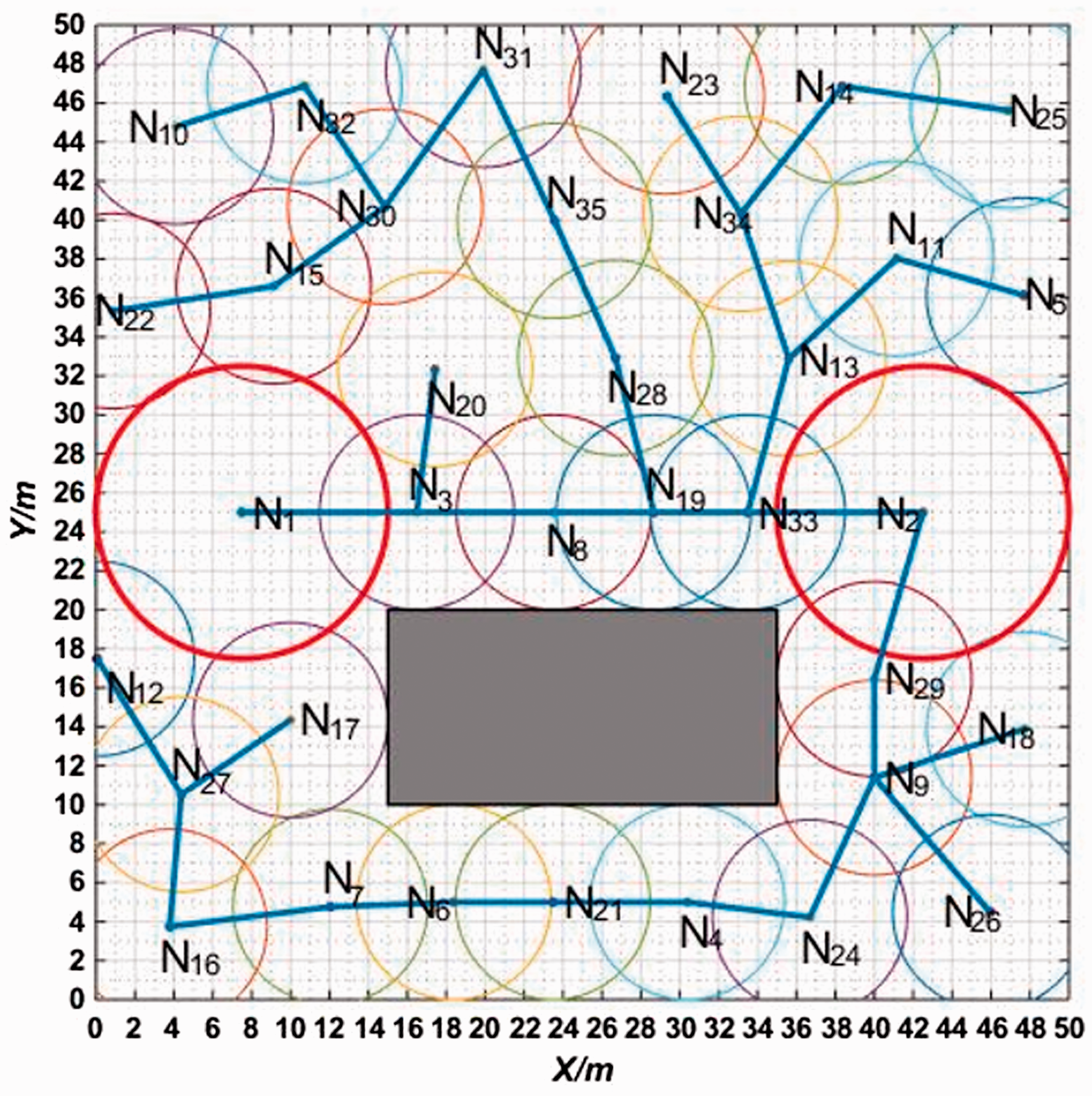
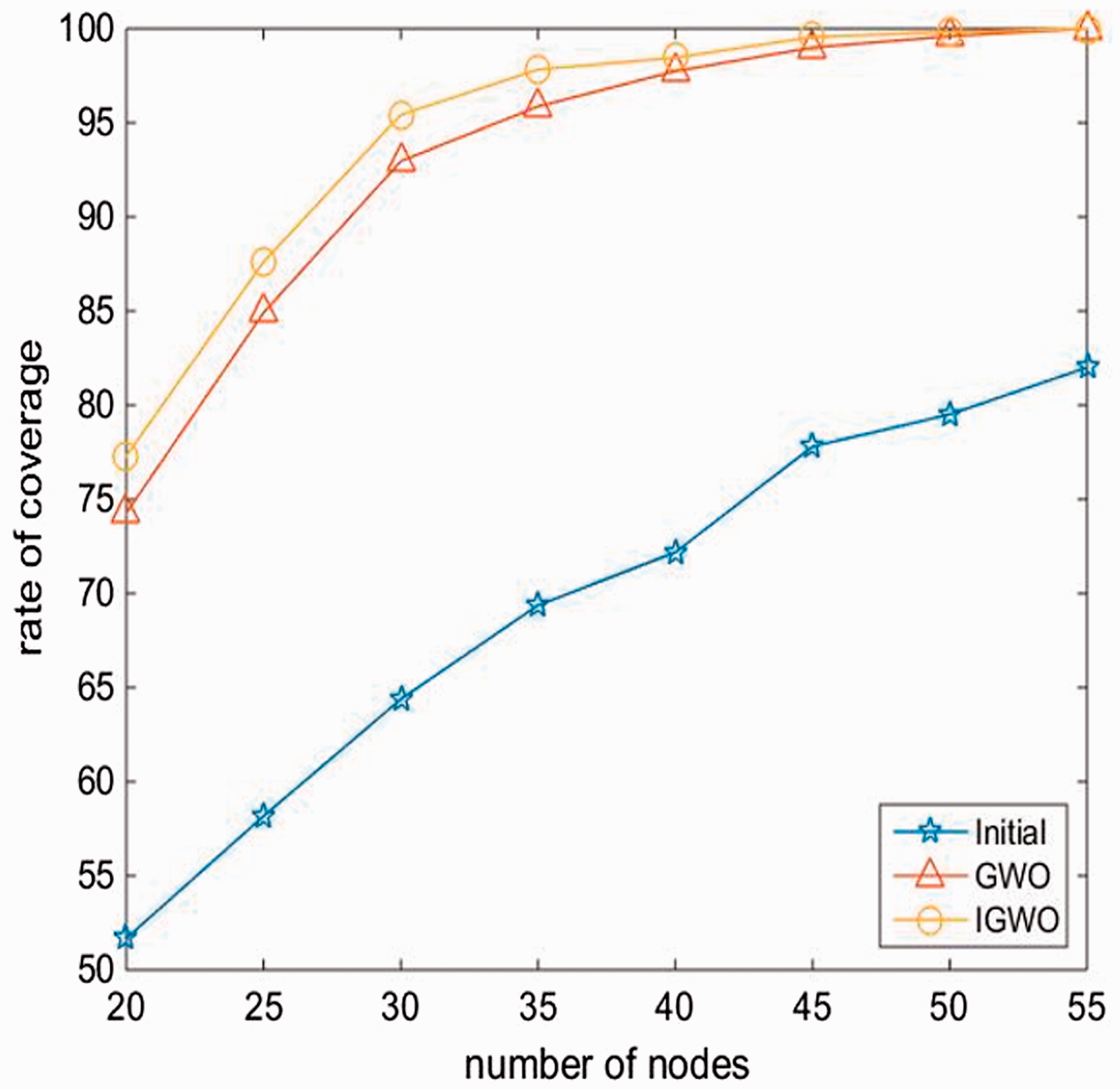
In order to better conform to the actual deployment environment of the sensor nodes, obstacles are set in the simulation environment, and the shapes are rectangle (200 m²), trapezoid (450 m²), and triangle (450 m²). Because of the low cost of sensor nodes, the mobility capability after deployment may be lost, so the mobile node will be converted into a static node, but its perceived radius will also increase. Figure 10 describes the coverage deployment scheme of IGWO algorithm in the presence of rectangular obstacles and the loss of mobility of two nodes. When the number of sensor nodes reaches 35, the coverage rate reaches to 97.83%. Figure 11 describes the comparison of the coverage rate of random, GWO, and IGWO deployment networks with different number of nodes. It can be seen that when the number of nodes is 55, the optimized coverage of the IGWO and GWO algorithms reaches to 100%, and the random coverage rate is only 82%. When the number of nodes is 30, the coverage rate of the IGWO algorithm reaches to 95.43%, which are 31.05% higher than random throwing and 2.47% higher than the GWO algorithm. It is worth noting that experiments have shown that the strategy of covering the circumference tangent to the obstacle is slightly higher than the strategy of the non-tangential strategy.

Figure 10.

IGWO optimized deployment.

Figure 11.

Number and coverage of nodes.

In the trapezoidal obstacle environment, the optimal deployment effect of the IGWO algorithm after 200 iterations at 30 nodes is shown in Figure 12, and the coverage rate reaches to 96.50%. Figure 13 shows the coverage rate comparison between the random algorithm, the GWO algorithm, and the IGWO algorithm when the number of nodes is different. At this time, the node coverage performance of IGWO is still better than the GWO algorithm, and the number of nodes to be deployed is less under the same coverage requirement. Finally, the node deployment scenario of the polygon monitoring area was tested. When the number of nodes is 30, the coverage of the network deployed with the IGWO algorithm reaches 95.63%, as shown in Figure 14. Figure 15 shows the node coverage performance of the random algorithm, GWO algorithm, and IGWO algorithm in the case of polygon monitoring area (triangular obstacles) with different number of nodes. It can be seen that the IGWO algorithm requires only 55 nodes to achieve 100% coverage, while the GWO algorithm requires 60 nodes. Therefore, 100% coverage can be achieved with fewer nodes, thereby saving network deployment costs. In the experiment of obstacle-free situation, the GWO and IGWO algorithms performed well. When the obstacles were added to the monitoring area, the monitoring area decreased, but the number of nodes required for the two algorithms to achieve 100% coverage is not reduced. It still need about 50–55 sensor nodes, which is due to obstacles in the monitoring area, the optimization complexity increases, and the optimization effect of the two is worse than the optimization effect in the case of no obstacles. However, from the performance of GWO algorithm and IGWO algorithm in different obstacle situations, IGWO algorithm has stronger adaptability to node optimization deployment in complex obstacle environment; in terms of achieving full coverage, irrespective of the shape of the obstacle; the IGWO algorithm can always achieve 100% coverage deployment with fewer nodes. This is because the dynamic mutation strategy enables the IGWO algorithm to dynamically adjust the position of the sensor nodes when they are deployed in a complex environment, so that they do not gather in the same area, thus avoiding the problem of local optimum. When the grey wolf boundary position strategy is applied to the node deployment, the sensor nodes that are not in the monitoring area due to the location update can be returned to the monitoring area; the distance between the node and the obstacle and the distance between the node and the boundary of the monitoring area are adjusted in a more reasonable manner, so that the network coverage becomes higher.

Figure 12.

IGWO optimized deployment.

Figure 13.

Number and coverage of nodes.

Figure 14.

IGWO optimized deployment.

Figure 15.

Number and coverage of nodes.

To sum up, in summary, compared with GWO, the superiority of IGWO algorithm benefits from the design of nonlinear convergence factor and elite strategy, so that the algorithm can achieve convergence effect in fewer iterations. And dynamic weighting strategy, grey wolf boundary position strategy and mutation strategy improve the precision of the algorithm. When the IGWO algorithm is applied to the optimal deployment of wireless sensor nodes, regardless of whether there are static nodes, whether there are obstacles, and what is the shape of the obstacle, the IGWO algorithm has a good effect on the coverage optimization problem of WSN nodes.

Conclusions

In order to solve the problem of optimal deployment of WSN nodes in complex environments, an improved algorithm IGWO is designed based on the standard GWO algorithm. In order to speed up the convergence of the algorithm, the elite strategy is introduced, and then nonlinear convergence factors are used to balance the global and local search capabilities of the algorithm. Original weighting strategy is improved, so that the dynamic update position is more in line with the original intention of the original algorithm. A grey wolf boundary position strategy is proposed, which increases the possibility of searching for the global optimal solution in the range, thus improving the precision of solution. The introduction of dynamic mutation strategy increases the diversity of wolves, effectively expands the search range of the algorithm, and solves the problem that the GWO algorithm is easy to fall into local optimum in the later stage. It is verified by simulation experiments on the test function that IGWO has a better convergence effect. When the IGWO algorithm is applied to WSN deployment, the simulation results show that the IGWO algorithm improves the coverage performance of WSN nodes, enables higher coverage rate with fewer nodes, and reduces network deployment costs.

Footnotes

Declaration of Conflicting Interests

The author(s) declared no potential conflicts of interest with respect to the research, authorship, and/or publication of this article.

Funding

The author(s) disclosed receipt of the following financial support for the research, authorship, and/or publication of this article: This work is supported by the National Natural Science Foundation of China (61562037, 61562038, 61563019, 61763017), the Natural Science Foundation of Jiangxi Province (20171BAB202026, 20181BBE58018), Science and Technology Project Founded by the Education Department of Jiangxi Province (GJJ150643), and Innovation Designated Fund for Graduate Student of Jiangxi Province (YC2018-S331).

ORCID iD

Zhendong Wang

References

Mini

Udgata

Sabat

SL.

Sensor deployment and scheduling for target coverage problem in wireless sensor networks. IEEE Sens J 2013; 14: 636–644.

Babaie

Pirahesh

SS.

Hole detection for increasing coverage in wireless sensor network using triangular structure. Int J Comput Sci 2012; 9: 672–673.

Huang

Kang

, et al. GA-based Sweep Coverage Scheme in WSN. In: International conference on cloud computing & big data, Macau, China, 16–18 November, 2016, pp.254–259. New York: IEEE.

Feng

JF.

The research of coverage algorithm for three-dimensional WSN based on MO-DMS-PSO. In: IEEE advanced information technology, electronic and automation control conference (IAEAC), Chongqing, China, 19–20 December 2015, pp.797–801. New York: IEEE.

Kumar

Gupta

and Benefits of using particle swarm optimization and Voronoi diagram for coverage in wireless sensor networks. In: International conference on emerging trends in computing and communication technologies (ICETCCT), Dehradun, India, 17–18 November 2017, pp.1–7. New York: IEEE.

Wang

Zhang

Fang

, et al. Research on probabilistic voronoi model and algorithm for coverage in WSN. Chin J Sens Actuat 2012; 25: 702–706.

Abo-Zahhad

Sabor

Sasaki

, et al. A centralized immune-Voronoi deployment algorithm for coverage maximization and energy conservation in mobile wireless sensor networks. Inform Fusion 2016; 30: 36–51.

Yao

A GA approach to the optimal placement of sensors in wireless sensor networks with obstacles and preferences. In: IEEE consumer communications & networking conference, Las Vegas, NV, USA, 8–10 January 2006, pp.127–131. New York: IEEE.

Liang

Lin

YH.

A coverage optimization strategy for mobile wireless sensor networks based on genetic algorithm. In: IEEE international conference on applied system invention (ICASI), Chiba, Japan, 13–17 April 2018, pp.1272–1275. New York: IEEE.

10.

Zorlu

Sahingoz

OK.

Increasing the coverage of homogeneous wireless sensor network by genetic algorithm based deployment. In: Digital information and communication technology and its applications (DICTAP), Konya, Turkey, 21–23 July 2016, pp.109–114. New York: IEEE.

11.

Cong

A coverage algorithm for WSN based on the improved PSO. In: International conference on intelligent transportation, big data and smart city, Halong Bay, Vietnam, 19–20 December 2015, pp.12–15. New York: IEEE.

12.

Yin

Guo

, et al. Research on coverage algorithm for wireless sensor networks based on improved particle swarm optimization algorithm. In: International conference on computer systems, electronics and control (ICCSEC), Dalian, China, 25–27 December 2017, pp.1207–1210. New York: IEEE.

13.

Mirjalili

Lewis

Grey wolf optimizer. Adv Eng Softw 2014; 69: 46–61.

14.

Kamboj

Bath

KandDhillon

JS.

Solution of non-convex economic load dispatch problem using grey wolf optimizer. Neural Comput Appl 2016; 27: 1301–1316.

15.

Kaveh

Zakian

Improved GWO algorithm for optimal design of truss structures. Eng Comput 2018; 34: 685–707.

16.

Pan

J-S

Dao

T-K

Chu

S-C.

A Novel Hybrid GWO-FPA Algorithm for Optimization Applications. In: Proceedings of the first international conference on smart vehicular technology, transportation, communication and applications, Kaohsiung, Taiwan, 6–8 November 2017, pp.27–281. Switzerland: Springer.

17.

Shieh

Wang

Dao

TK.

Enhanced diversity herds grey wolf optimizer for optimal area coverage in wireless sensor networks. In: International conference on genetic and evolutionary computing, Fuzhou, China, 7–9 November 2016, pp.174–182. Switzerland: Springer.

18.

Madadi

Motlagh

MM.

Optimal control of DC motor using grey wolf optimizer algorithm. Tech J Eng Appl Sci 2014; 4: 373–379.

19.

Mesbahi

Egerstedt

Graph theoretic methods in multiagent networks. Princeton: Princeton University Press, 2010, vol. 33.

20.

Zhou

Chen

, et al. Kruskal algorithm based assessment on power system structural vulnerability. Power Syst Technol 2013; 37: 3172–3177.

21.

Wen

Tie-Bin

WU.

Improved grey wolf optimization algorithm coordinating the ability of exploration and exploitation. Cont Decision 2017; 32: 1749–1757.

22.

Tao

Chen

Adaptive differential evolution with multi-population-based mutation operators for constrained optimization. Soft Comput 2019; 23: 3423–3447.

23.

Ahn

Ramakrishna

RS.

Elitism-based compact genetic algorithms. IEEE T Evolut Comput 2003; 7: 367–385.

24.

Yang

Yuan

, et al. A modified particle swarm optimizer with dynamic adaptation. Appl Math Comput 2007; 189: 1205–1213.

Node coverage optimization algorithm for wireless sensor networks based on improved grey wolf optimizer

Abstract

Keywords

Introduction

Model description

Network coverage model

Network connectivity model

Standard GWO algorithm

Social hierarchy

Round up hunting

Algorithm 1: grey wolf optimizer

Improved GWO algorithm

Nonlinear convergence factor strategy

Elite strategy

Dynamic weighting strategy

Dynamic variation strategy

Grey wolf boundary position strategy

Improved grey wolf algorithm description

Algorithm complexity analysis

Simulation experiments

Experiment 1—comparison of algorithm convergence

Experiment 2—comparison of node coverage

Conclusions

Footnotes

Declaration of Conflicting Interests

Funding

ORCID iD

References