Noninvasive Quantification of Local Cerebral Metabolic Rate of Glucose for Clinical Application Using Positron Emission Tomography and 18 F-Fluoro-2-Deoxy- d -Glucose

Abstract

Until now, input function is still required in quantification of local cerebral metabolic rate of glucose (LCMRGlc) using positron emission tomography (PET) and ¹⁸F-fluoro-2-deoxy-d-glucose (FDG). Some image-derived methods were developed to get input function noninvasively instead of the arterial blood sampling method, but they needed to make complicated corrections manually, so they cannot always be applied in clinic directly. Here, we propose a simple method based on the Patlak approach by using a reference tissue region and without using any information of input function. This simulation study revealed that the present method was in good agreement with Patlak method; the difference between two methods was less than 5%. The statistical errors with two methods were also obtained, and the results showed the accuracy of LCMRGlc estimated with present method was better than that with Patlak method slightly. The simulation results indicated that the calculation of LCMRGlc with present method was quite stable and independent of the choosing of reference tissue region. All of these show that the present method is a good approximation to Patlak method. The calculation with this method is very simple and easy to perform voxel by voxel; therefore, it can be widely used not only in laboratory studies but also in clinical applications although it only provides the relative rates.

Introduction

Local cerebral metabolic rate of glucose (LCMRGlc) is an important index to embody the neural function, using ¹⁸F-fluoro-2-deoxy-D-glucose (FDG), as the tracer with positron emission tomography (PET) becomes one of the most widely used noninvasive methods for quantification of LCMRGlc in humans (Phelps et al, 1979; Reivich et al, 1979). In quantification of LCMRGlc with PET/FDG, the plasma time—activity curve (PTAC) is required and used as the input function. In the early studies, the PTACs are usually obtained by taking arterial or arterialized venous blood samples invasively (Phelps et al, 1979; Huang et al, 1980). The arterial blood sampling needs inserting arterial lines; it is quite invasive and causes the patient discomfort, involves potential risks of arterial thrombosis, arterial sclerosis, and ischemia to the distal extremity (Chen et al, 1998). The acquirement and processing of arterial blood is also incompatible in the PET study or its clinical application; it requires extra personnel to process, exposes personnel to the risks associated with the handling of patient blood and increased radiation from proximity to the patient (Correia, 1992), and needs additional laboratory procedures for measuring the blood samples and calibrating the equipment. This kind of LCMRGlc quantification is not always performed in PET/FDG practices.

Owing to the disadvantages associated with the arterial or arterialized blood samples, some methods have been developed to minimize or eliminate the invasive blood sampling procedure in PET studies of brain and other organs. Most of the useful methods are using the time—activity curve obtained from an region of interest (ROI) drawn on the vascular structure over the PET images as the input function, therefore this kind of input function is also named as the image-derived input function (Chen et al, 1998). These techniques are well used in cardiac PET studies (Weinberg et al, 1988; Gambhir et al, 1989; Iida et al, 1992), hepatic and renal PET studies (Germano et al, 1992; Chen et al, 1992), and brain PET studies (Chen et al, 1998; Parker and Feng, 2005), in which the input functions are obtained by selecting an ROI within the cavity of the left ventricle, the abdominal aorta, and the internal carotid arteries, respectively. However, when the tracer starts gathering in the adjacent tissue, the spillover from tissue-to-blood aggravates and should be corrected. The partial volume effects induced by the small size of these ROI should also be raveled out. In correcting spillover and partial volume effects, some venous blood samples are still required. Owing to the PET data itself and the need to make corrections for above effects, the input functions obtained with these methods are extremely noisy; therefore, the direct use of such input functions in FDG dynamic model increases the statistical uncertainties in the estimated model parameters such as LCMRGlc (Lin et al, 1992). As the complete time course of the input function is needed in making above corrections and the input function changes immediately in the early stage after the bolus tracer injection, it needs a fast image-acquisition protocol and causes added manipulations.

To solve the problems with the image-derived input function, an analytical model of the input function (Feng et al, 1993; Phillips et al, 1995) or a template calculated from a sample population (Takikawa et al, 1993) was applied. Because these PTAC models were based on other FDG experimental data obtained from blood samples of the population, the input function of single subject can be determined by estimating a few model parameters. With the template, the input function of single subject can be replaced by that of the population. However, because there are many differences in individual physiologic states (e.g., cardiac output) and procedural factors (e.g., the injection rate), it is hard to use a simple model or uniform pattern to describe the shape of the input function. As the modeling method still needs some blood samples of the subject to estimate PTAC parameters, and the sampling number depends on the parameter number, more reliable model needs more parameters. Therefore if one has to get true input function, this method cannot reduce the blood sampling number drastically. In addition, the template may also not match well with special data of the patient. Therefore, all the methods including arterial blood sampling, image-derived, and modeling (or template) method for input function cannot simply be used to quantify LCMRGlc in clinical case.

Because the input function is a common factor for the tissue time—activity curve (TTAC, also defined as output function) in tracer dynamic models, it is assumed that the input function is uniform for all TTACs in different regions of brain. Therefore using multiequations for TTACs of these different regions, this common factor can be removed and the model parameters can be estimated without using the input function. This method has been applied successfully in quantification of the cerebral blood flow using PET with ¹⁵O-water (Mejia et al, 1994; Watabe et al, 1996), whose kinetics is described by a single-compartment model. Because the kinetics of FDG is more complex than that of ¹⁵O-water, this method cannot be used for FDG directly. However by considering Patlak graphical approximation (Patlak et al, 1983; Patlak and Blasberg, 1985) we propose a similar approach for the quantification of LCMRGlc with PET/FDG. The method uses two TTACs from two different regions and is noninvasive completely. It requires neither arterial blood, nor corrections for the spillover and partial volume when using image-derived input function. Unlike methods using an arterial input function, only the relative net FDG clearance can be estimated using the present method without other constraints. However, even after removing the global effect, this method will still be able to produce functional images of LCMRGlc pixel by pixel with short calculation times, and can also be carried out automatically without needing manual operation. ¹⁸F-Fluoro-2-deoxy-d-glucose is commonly used with PET to image metabolic states for diagnosis of brain and heart disease as well as cancer and other disease. The accuracy of clinical diagnosis depends on whether and how the PET data are quantified to the physiologic value. Therefore this method can also be used for the daily clinical diagnosis instead of using tissue radioactivity or its homomorphism—standard uptake value.

Theory

The present method is based on the Patlak graphical approach (Patlak et al, 1983; Patlak and Blasberg, 1985), in which the relationship between tissue radioactivity concentration and arterial input function can be described as follows:

$$c_{\mathrm{i}}^{*}(t)=K{\int }_0^t{c}_{\mathrm{p}}^{*}(\tau )\mathrm{d}\mathrm{\tau }+W{c}_{\mathrm{p}}^{*}(t),\hspace{0.17em}\hspace{0.17em}t>t_0$$

(1)

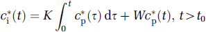
where c_i*(t) and C_p*(t), respectively, reflect the radioactive FDG concentrations at time t in the brain tissue and arterial blood, K is the net FDG clearance from blood to tissue (Kuwabara et al, 1990) and is used to calculate LCMRGlc (R = (c_p/LC)K, where c_p is the glucose concentration in the plasma, LC is the lumped constant, which summarizes the difference between FDG and glucose in transportation and phosphorylation) (Sokoloff et al, 1977; Huang et al, 1980), W is another constant related to the steady-state volume of the reversible compartments and effective plasma volume (Patlak and Blasberg, 1985). Both c_i*(t) and c_p*(t) are decay-corrected.

Arbitrarily choosing two regions called reference region and objective region in brain (or other organs), equation (1) can be described for both regions as follows:

$$c_{\text{ir}}^{*}(t)=K_{\mathrm{r}}{\int }_0^t{c}_{\mathrm{p}}^{*}(\tau )\mathrm{d}\tau +W_{\mathrm{r}}{c}_{\mathrm{p}}^{*}(t),\hspace{0.17em}\hspace{0.17em}t>t_0$$

(2)

$$c_{\text{io}}^{*}(t)=K_{\mathrm{o}}{\int }_0^t{c}_{\mathrm{p}}^{*}(\tau )\mathrm{d}\tau +W_{\mathrm{o}}{c}_{\mathrm{p}}^{*}(t),\hspace{0.17em}\hspace{0.17em}t>t_0$$

(3)

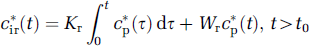
where the subscript ‘r’ and ‘o’ denote the reference region and objective region, respectively. It is assumed that the input function c_p*(t) is same for all regions in brain.

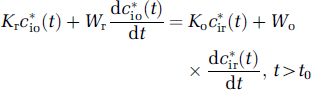
It is easy to get equation (4) from equations (2) and (3). Then rearranging and integrating equation (4) from time t₀ to t gives the equation (5)

$$\begin{array}{l}{K}_{\mathrm{r}}{C}_{\text{io}}^{*}(t)+W_{\mathrm{r}}\frac{\mathrm{d}{c}_{\text{io}}^{*}(t)}{\mathrm{d}t}=K_{\mathrm{o}}{C}_{\text{ir}}^{*}(t)+W_{\mathrm{o}}\\ \times \frac{\mathrm{d}{c}_{\text{ir}}^{*}(t)}{\mathrm{d}t},t>t_0\end{array}$$

(4)

$$\begin{array}{l}{\int }_{t_0}^t{c}_{\text{io}}^{*}(\tau )\mathrm{d}\tau =\frac{K_{\mathrm{o}}}{K_{\mathrm{r}}}{\int }_{t_0}^t{c}_{\text{ir}}^{*}(\tau )\mathrm{d}\tau +\frac{W_{\mathrm{o}}}{K_{\mathrm{r}}}(c_{\text{ir}}^{*}(t)-c_{\text{ir}}^{*}(t_0))\\ +\frac{W_{\mathrm{r}}}{K_{\mathrm{r}}}(c_{\text{io}}^{*}(t_0)-c_{\text{io}}^{*}(t)),t>t_0\end{array}$$

(5)

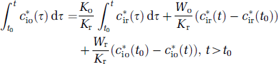
where t₀ is the time of the first used frame for PET scan after FDG injection. Recall that the equation (1) is an approximation to the FDG dynamic model (see Materials and methods) in the time region greater than t₀, where t₀ is approximately 10 mins; therefore all equations derived from equation (1) is also approximate and validated in the time region greater than t₀ only. To simplify the expression, ‘t > t₀‘ will be ignored in subsequent equations concerning to this.

In equations (4) and (5), the arterial input function c_p*(t) has been eliminated. Denoting K_or = K_o/K_r (the relative net FDG clearance in objective region to reference region), W_rr = W_r/K_r and W_or = W_o/K_r, equation (5) can be rewritten simply as

$$\begin{array}{l}{\int }_{t_0}^t{c}_{\text{io}}^{*}(\tau )\mathrm{d}\tau =K_{\text{or}}{\int }_{t_0}^t{c}_{\text{ir}}^{*}(\tau )\mathrm{d}\tau +W_{\text{or}}(c_{\text{ir}}^{*}(t)-c_{\text{ir}}^{*}(t_0))\\ +W_{\text{rr}}(c_{\text{io}}^{*}(t_0)-c_{\text{io}}^{*}(t))\end{array}$$

(6)

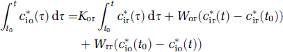
Taking digitized samples at time t₀, t₁,…, t_n (t₀, t₁,…, t_n are the sampling times of PET scans used), n equations based on equation (6) are obtained

$$\{\begin{array}{l}{\int }_{t_0}^{t_1}{c}_{\text{io}}^{*}(\tau )\mathrm{d}\tau =K_{\text{or}}{\int }_{t_0}^{t_1}{c}_{\text{ir}}^{*}(\tau )\mathrm{d}\tau +W_{\text{or}}(c_{\text{ir}}^{*}(t_1)-c_{\text{ir}}^{*}(t_0))\\ +W_{\text{rr}}(c_{\text{io}}^{*}(t_0)-c_{\text{io}}^{*}(t_1))+{\epsilon }_1\\ {\int }_{t_0}^{t_2}{c}_{\text{io}}^{*}(\tau )\mathrm{d}\tau =K_{\text{or}}{\int }_{t_0}^{t_2}{c}_{\text{ir}}^{*}(\tau )\mathrm{d}\tau +W_{\text{or}}(c_{\text{ir}}^{*}(t_2)-c_{\text{ir}}^{*}(t_0))\\ +W_{\text{rr}}(c_{\text{io}}^{*}(t_0)-c_{\text{io}}^{*}(t_2))+{\epsilon }_2\\ ⋮\\ {\int }_{t_0}^{t_n}{c}_{\text{io}}^{*}(\tau )\mathrm{d}\tau =K_{\text{or}}{\int }_{t_0}^{t_{\mathrm{n}}}{c}_{\text{ir}}^{*}(\tau )\mathrm{d}\tau +W_{\text{or}}(c_{\text{ir}}^{*}(t_n)-c_{\text{ir}}^{*}(t_0))\\ +W_{\text{rr}}(c_{\text{io}}^{*}(t_0)-c_{\text{io}}^{*}(t_n))+{\epsilon }_n\end{array}$$

(7)

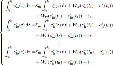
where ε₁, ε₂,…, ε_n are the equation error terms. Because the integration term of c_i*(t) exists in equation (7), the errors of these equations are not independent of each other even though the measurement errors of c_i*(t) are independent. They are a set of linear equations about three parameters of K_or, W_rr, and W_or. Let

$$\begin{array}{l}\theta =[\begin{array}{l}{K}_{\text{or}}\\ W_{\text{or}}\\ W_{\text{rr}}\end{array}],\hspace{0.17em}\hspace{0.17em}Y=\left[\begin{array}{l}{\int }_{t_0}^{t_1}{c}_{\text{io}}^{*}(\tau )\mathrm{d}\tau \\ {\int }_{t_0}^{t_1}{c}_{\text{io}}^{*}(\tau )\mathrm{d}\tau \\ ⋮\\ {\int }_{t_0}^{t_n}{c}_{\text{io}}^{*}(\tau )\mathrm{d}\tau \end{array}\right],\hspace{0.17em}\hspace{0.17em}\epsilon =\left[\begin{array}{l}{\epsilon }_1\\ {\epsilon }_1\\ ⋮\\ {\epsilon }_n\end{array}\right],\\ X=\left[\begin{array}{l}{\int }_{t_0}^{t_1}{c}_{\text{ir}}^{*}(\tau )\mathrm{d}\tau \hspace{0.17em}\hspace{0.17em}{c}_{\text{ir}}^{*}(t_1)-c_{\text{ir}}^{*}(t_0)\hspace{0.17em}\hspace{0.17em}{c}_{\text{io}}^{*}(t_0)-c_{\text{io}}^{*}(t_1)\\ {\int }_{t_0}^{t_2}{c}_{\text{ir}}^{*}(\tau )\mathrm{d}\tau \hspace{0.17em}\hspace{0.17em}{c}_{\text{ir}}^{*}(t_2)-c_{\text{ir}}^{*}(t_0)\hspace{0.17em}\hspace{0.17em}{c}_{\text{io}}^{*}(t_0)-c_{\text{io}}^{*}(t_2)\\ ⋮⋮⋮\\ {\int }_{t_0}^{t_n}{c}_{\text{ir}}^{*}(\tau )\mathrm{d}\tau \hspace{0.17em}\hspace{0.17em}{c}_{\text{ir}}^{*}(t_n)-c_{\text{ir}}^{*}(t_0)\hspace{0.17em}\hspace{0.17em}{c}_{\text{io}}^{*}(t_0)-c_{\text{io}}^{*}(t_n)\end{array}\right],\end{array}$$

Equation (7) can be rearranged into a matrix form:

$$Y=X\theta +\epsilon$$

(8)

Therefore the parameters K_or, W_rr, and W_or will be estimated easily and quickly from equation (8) using linear least-squares method

$${\theta }_{\text{LLS}}={(X^{T}X)}^{-1}{X}^{T}Y$$

(9)

In equation (9), no information regarding input function was needed. Although K_or is defined in the ROI, it can also be calculated pixel by pixel if a pixel is selected as an ROI. It is worth mentioning here that using equations (2) and (3), K_o, W_o, and K_r, W_r can be calculated, respectively. As the comparison, K_or, W_rr, and W_or can be estimated with Patlak method too, but as described above, it needs input functions.

Materials and methods

To reflect the real situation, TTACs c_i*(t) were generated using three-compartmental model (equation (10)), the FDG dynamic model (Huang et al, 1980):

$$c_{\mathrm{i}}^{*}(t)=(B_1{\mathrm{e}}^{-{\alpha }_{1}t}+B_2{\mathrm{e}}^{-{\alpha }_{2}t})\otimes c_{\mathrm{p}}^{*}(t)$$

(10)

where ⊗ denotes operation of convolution,

$$\begin{array}{l}{B}_1=k_1^{*}(k_3^{*}+k_4^{*}-{\alpha }_1)/({\alpha }_2-{\alpha }_1),\\ B_2=k_1^{*}({\alpha }_2+k_3^{*}-k_4^{*})/({\alpha }_2-{\alpha }_1),\\ {\alpha }_1=\frac{1}{2}(k_2^{*}+k_3^{*}+k_4^{*}\sqrt{{(k_2^{*}+k_3^{*}+k_4^{*})}^2-4k_2^{*}{k}_4^{*}}),\\ {\alpha }_2=\frac{1}{2}(k_2^{*}+k_3^{*}+k_4^{*}\sqrt{{(k_2^{*}+k_3^{*}+k_4^{*})}^2-4k_2^{*}{k}_4^{*}}),\end{array}$$

k₁*, k₂*, k₃*, and k₄* are the transport rate constants, and c_p*(t) is the input function.

In this computer simulation study, a PTAC model was used to generate the input function curve. We used the following equation, proposed in Feng et al (1993), to generate the plasma time—activity input function, c_p*(t):

$$c_{\mathrm{p}}^{*}(t)=[A_{1}t-A_2-A_3]{\mathrm{e}}^{{\lambda }_{1}t}+A_2{\mathrm{e}}^{{\lambda }_{2}t}+A_3{\mathrm{e}}^{{\lambda }_{3}t}$$

(11)

where λ₁, λ₂, and λ₃ are the eigenvalues and A₁, A₂, and A₃ are the coefficients of the model. A typical c_p*(t) is shown in Figure 1 using the following values: A₁ = 851.1225, A₂ = 20.8113, and A₃ = 21.8798 (μCi/mL), and λ₁ = −4.133859, λ₂ = −0.01043449, and λ₃ = −0.1190996 (min⁻¹). As these coefficient values and eigenvalues are derived from real FDG PTAC input function studies (Feng et al, 1993), this input function reflects also the real situation.

Figure 1

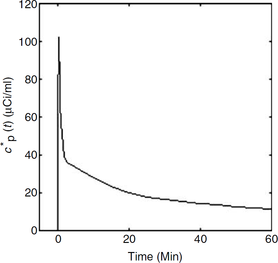
Typical plasma time-activity curve. The horizontal axis is time in minutes. The vertical axis is the radioactivity in μCi/mL.

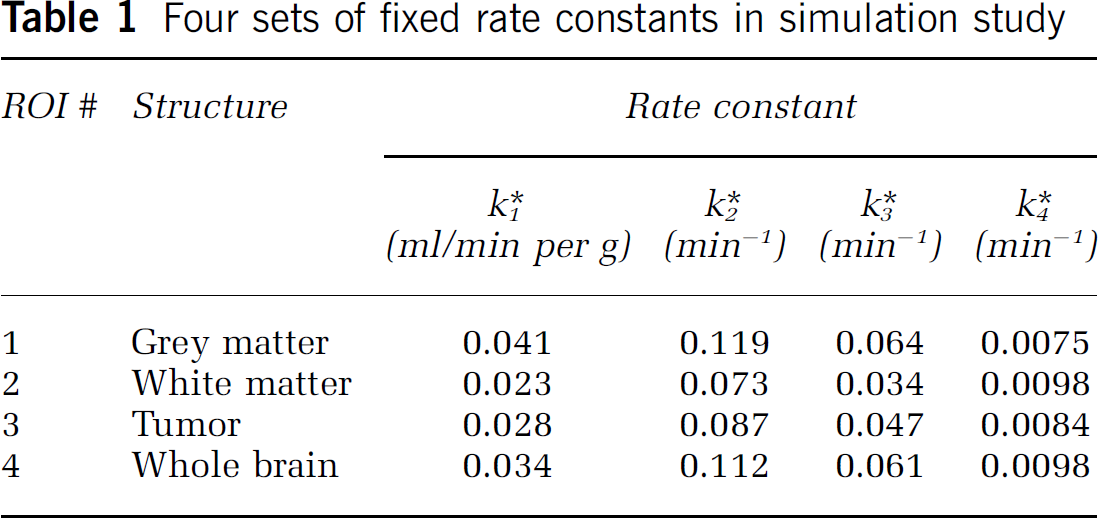
To simulate the real situation, the pseudorandom number of the rate constants k₁*, k₂*, k₃*, and k₄* were generated with continuous uniform distribution, in which the interval of each constant were taken as 0.015 < k₁* < 0.286, 0.024 < k₂* < 0.546, 0.010 < k₃* < 0.192, and 0.0014 < k₄* < 0.0186. They are based on the experimental results of Huang et al (1980) for both grey and white matters in human brain from 13 subjects. The upper limits of these rate constants were double their maximum values in the literature (Huang et al, 1980) and the lower limits were half their minimum values. The TTACs were calculated using equation (10) by using the above c_p*(t) values, above random rate constants and other four sets of typical transport rate constants obtained in human study (Hawkins et al, 1986), as shown in Table 1.

Table 1

Four sets of fixed rate constants in simulation study

ROI #	Structure	Rate constant
		k1* (ml/min per g)	k2* (min−1)	k3* (min−1)	k4* (min−1)
1	Grey matter	0.041	0.119	0.064	0.0075
2	White matter	0.023	0.073	0.034	0.0098
3	Tumor	0.028	0.087	0.047	0.0084
4	Whole brain	0.034	0.112	0.061	0.0098

In this study, because the proposed method does not use the input function, and only the effects of PET measurement noise was considered, we did not add any errors to input function in the Patlak method as comparison. The Gaussian noises were added on TTACs using a pseudorandom number generator, in which the mean value of random number was zero and the error variance was calculated from the following equation (Feng et al, 1995):

$${\sigma }^2(t_j^{\prime })=\alpha \times {\bar{c}}_{\mathrm{i}}^{*}(t_j^{\prime })/\delta t_j$$

(12)

where α is the noise level and was set to 0 (noise-free), 0.1, 0.5, 1.0, 2.0, and 4.0, respectively; c⁻_i* (t′_j) = ∫_tj-1^t_j c_i* (τ) dτ/δt_j is the average value of c_i*(t) over the length of the jth scanning interval, t′_j = (t_j–1 + t_j)/2 and δt_j = t_j–t_j–1 is the length of jth scanning interval.

Results

We defined five kinds of ROI in Materials and methods, one of them is generated with FDG dynamic model using the random rate constants k and denoted by subscript p. The rate constants k in this kind of ROI were taken randomly and used to represent different tissue (because we did not perform the real PET experiment, we require this kind of ROI to reflect the real situation). Other four ROIs are generated using four sets of fixed rate constants k listed in Table 1 and denoted by their ROI# as the subscript, they play the role of reference region to first kind of ROI or themselves. As the first and last subscripts of K also denote the objective region and reference region, respectively, K_ij (i, j = 1, 2, 3, 4, i ≠ j) indicates the relative net FDG clearance in ROI #i to ROI #j and K_pi (i = 1, 2, 3, 4) indicates the relative net FDG clearance in the ROI generated with random rate constants to the ROI #i. Five thousand event data for each set of TTACs were generated with each noise level. Finally there are 5 × 6 groups data set. For each TTAC, there were 11 scanning intervals starting from 5 mins after FDG injection, and each frame lasted 5 mins.

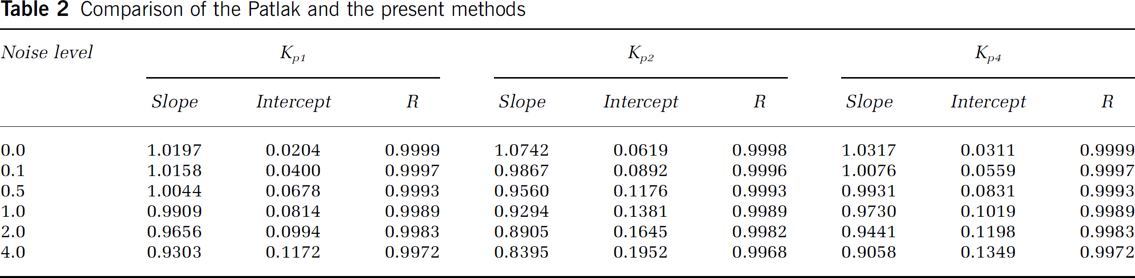
To check the correlation between different calculations of K_or (the relative net FDG clearance), the linear regression y = Sx + I was carried out using weighted least-squares method, in which the weight was taken as (x² + y²), where y and x are the two K_or values calculated using two methods, S is the slope and I is the intercept. Figure 2 is an example of the correlation between two values of K_p1 estimated with Patlak method and the present method with noise level α = 1.0. Similar results were obtained and are shown in Table 2 for other such comparisons. Table 2 gives the slope, intercept, and correlation coefficient (R) for the comparison between Patlak and the present methods with six different noise levels. The slopes are close to unity, the intercepts are close to 0, and the correlation coefficients are very close to 1; this implies that the two methods are very similar. As mentioned above, the Patlak method is an approximation to the FDG dynamic model; the present and Patlak method are also not equivalent exactly for real FDG data. Therefore even in the absence of noise, there still exists small difference between the K_or values estimated using these two methods.

Table 2

Comparison of the Patlak and the present methods

Noise level	Kp1			Kp2			Kp4
	Slope	Intercept	R	Slope	Intercept	R	Slope	Intercept	R
0.0	1.0197	0.0204	0.9999	1.0742	0.0619	0.9998	1.0317	0.0311	0.9999
0.1	1.0158	0.0400	0.9997	0.9867	0.0892	0.9996	1.0076	0.0559	0.9997
0.5	1.0044	0.0678	0.9993	0.9560	0.1176	0.9993	0.9931	0.0831	0.9993
1.0	0.9909	0.0814	0.9989	0.9294	0.1381	0.9989	0.9730	0.1019	0.9989
2.0	0.9656	0.0994	0.9983	0.8905	0.1645	0.9982	0.9441	0.1198	0.9983
4.0	0.9303	0.1172	0.9972	0.8395	0.1952	0.9968	0.9058	0.1349	0.9972

Figure 2

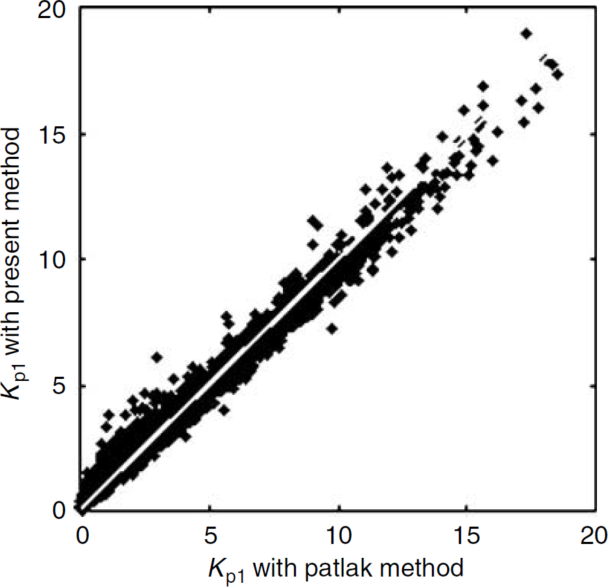
The correlation of K_P1 (ROI #1 is the reference region) calculated using the Patlak method (abscissa) and the present method (ordinate) with noise level α = 1.0. The white solid line among scattering dots is the regression line.

According to K_or = K_o/K_r and K_ro = K_r/K_o, the product of these two parameters should be equal to 1. If objective and reference region are exchanged with each other in equation (6), two equations are obtained. If equation (6) is exact one, these two equations will be equivalent and this requirement will also be satisfied spontaneously, however, since equation (6) is only an approximate equation, K_or and K_ro are two parameters estimated using present method from two different equations, they will not be always satisfied with this requirement. K_or and K⁻¹_ro (the inverse of K_ro) have been compared. Figure 3 is an example of such correlation for K_p4 and K⁻¹_4p with noise level α = 2.0. Similar results were obtained and are shown in Table 3 for other such comparisons. Figure 3 and Table 3 show that with six different noise levels the slope, intercept, and correlation coefficients are very close to 1, 0, and 1, respectively, which means irrespective of which ROIs is taken as reference region, the results estimated using the present method will still be very consistent.

Table 3

Comparison of K_pi and the inverse of K_ip (i = 1, 2, 4)

Noise level	Kp1 versus K−11p			Kp2 versus K−12p			Kp4 versus K−14p
	Slope	Intercept	R	Slope	Intercept	R	Slope	Intercept	R
0.0	1.0013	0.0056	1.0000	1.0019	0.0012	1.0000	0.9986	–0.0035	1.0000
0.1	1.0034	0.0083	1.0000	1.0072	0.0018	1.0000	0.9956	–0.0070	1.0000
0.5	1.0065	0.0123	0.9999	1.0132	0.0032	1.0000	0.9904	–0.0093	1.0000
1.0	1.0096	0.0114	0.9999	1.0189	0.0018	1.0000	0.9864	–0.0081	1.0000
2.0	1.0137	0.0106	0.9999	1.0255	0.0015	0.9999	0.9815	–0.0078	0.9999
4.0	1.0213	0.0071	0.9999	1.0307	0.0061	0.9999	0.9735	–0.0062	0.9999

Figure 3

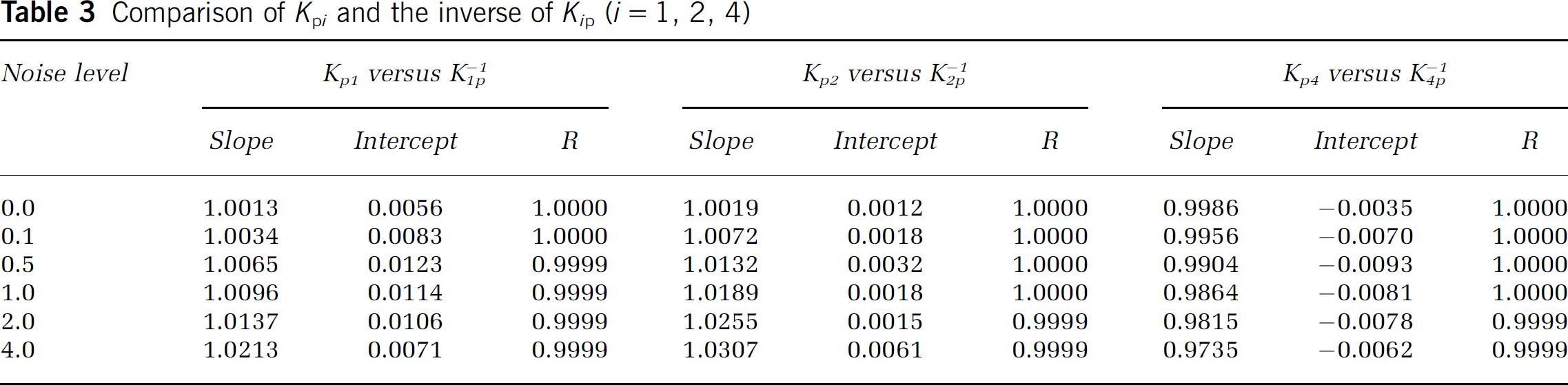
The correlation of K_p4 and K⁻¹_4p with noise level α = 2.0. The white solid line among scattering dots is the regression line.

Defining $r{K}_{ij}=\frac{K_i/K_m}{K_j/K_m}=\frac{K_i}{K_j}=K_{ij}$ . However, like K_or and K⁻¹_ro, rK_ij is not always equal to K_ij when using the present method to estimate them. Figure 4 is an example of such a correlation for K_p2 and rK_p2 with noise level α = 4.0. Similar results were obtained and are shown in Table 4 for other such comparisons. Figure 4 and Table 4 show that with six different noise levels, the slope, intercept, and correlation coefficients are also very close to 1, 0, and 1, respectively, this also means present method is a very consistent one.

Table 4

Comparison of K_pi and rK_pi (i = 1, 2, 4)

Noise level	KpI versus rKp1			Kp2 versus rKp2			Kp4 versus rKp4
	Slope	Intercept	R	Slope	Intercept	R	Slope	Intercept	R
0.0	0.9238	0.0041	1.0000	1.0213	–0.0094	0.9999	0.9739	0.0076	0.9999
0.1	1.0017	0.0052	1.0000	0.9802	–0.0043	1.0000	1.0176	0.0042	1.0000
0.5	1.0012	0.0015	0.9999	0.9813	0.0068	0.9999	1.0138	–0.0025	0.9999
1.0	0.9993	0.0012	0.9998	0.9796	0.0104	0.9998	1.0131	–0.0041	0.9998
2.0	0.9982	–0.0006	0.9998	0.9804	0.0105	0.9997	1.0091	–0.0030	0.9998
4.0	0.9953	0.0003	0.9997	0.9854	0.0031	0.9997	1.0006	0.0038	0.9997

Figure 4

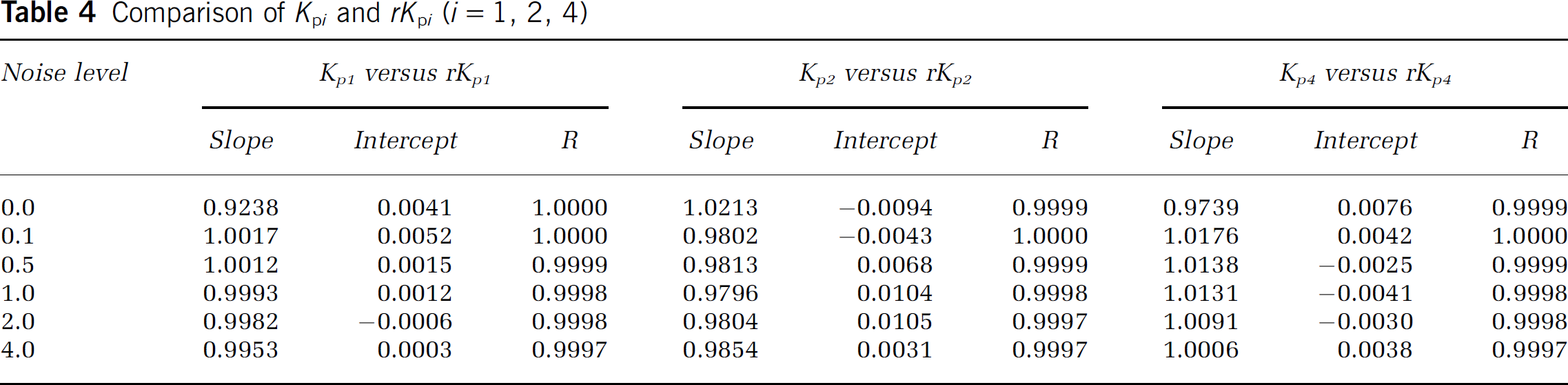
The correlation of K_p2 and rK_p2 with very high noise level α = 4.0. The white solid line among scattering dots is the regression line.

Using the four set of TTACs generated with fixed rate constants listed in Table 1, the difference between two K_or (o, r = 1, 2, 3, 4, o > r) values estimated with the Patlak method and the present method as well as their relative errors were got. The simulation results show that K_or obeys Gaussian distribution; by fitting line shapes of their distributions, the mean, and standard error were derived. Figure 5 shows that up to very high noise level (α = 4.0) the ratios of K_or estimated using the two methods are still close to 1 and the relative differences are less than 5%. Figure 6 shows that the relative errors with two methods changed increasingly with noise level, but the errors using the present method was less than those with the Patlak method. This indicates that the present method is a good approximation to Patlak method.

Figure 5

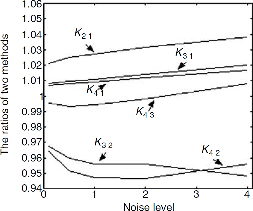
The ratios of K_or (o, r = 1, 2, 3, 4, o > r) values estimated by using the Patlak and the present methods against the noise level.

Figure 6

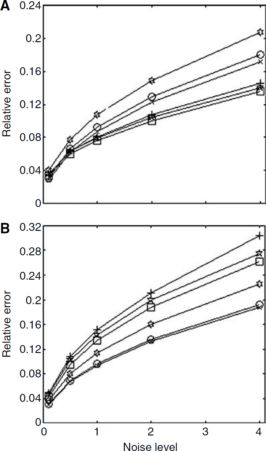
The relative errors changed with noise level for K_or (o, r = 1, 2, 3, 4, o > r) estimated by using (A) the present method and (B) the Patlak method. —▢—, K₂₁;—○—, K₃₁; — × —, K₄₁; — + —, K₃₂; —⋆—, K₄₂; — □ —, K₄₃.

Discussion and Conclusion

The above results show that the relative net FDG clearance in one ROI compared to the other can beestimated using the present method as a good approximation to the Patlak approach. Without other constraints, the absolute value of net FDG clearance cannot be calculated using the present method, this is the main drawback of this kind of reference method. In Watabe et al (1996), a quantitative absolute blood flow was estimated under the constraint that the distribution volume of water for all pixels within 10% of the maximum counts was fixed to 0.86 ml/ml. This assumption might be reasonable, but when comparing mean regional cerebral blood flow values of 17 subjects calculated using the dynamic/integral method and their method, the disagreement between the two methods in the high-flow study is not too small; this might be induced by the above assumption.

As the ROI is chosen as reference is not important in the present method, the simple way is to allow the whole brain (e.g., ROI#4 listed in Table 1) as the reference ROI. According to Sokoloff et al (1977) and Huang et al (1980), the LCMRGlc is

$$R=\frac{c_{\mathrm{p}}}{LC}K$$

(13)

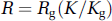
the global metabolic rate of glucose (GCMRGlc) is equal to R_g = (c_p/LC)K_g, where c_p is the glucose concentration in the plasma, LC is the lumped constant, and K and R_g are the net FDG clearances in local area and whole brain, respectively. Assuming LC is uniform in brain, equation (13) becomes to

$$R=R_{\mathrm{g}}(K/K_{\mathrm{g}})$$

(14)

where K/K_g is the relative net FDG clearance in local area to whole brain and can easily estimated using present method. Equations (13) and (14) can be used to calculate the LCMRGlc: equation (13) requires constant parameter LC, c_p, and net FDG clearance (K) in local area, and equation (14) requires constant parameter R_g and the relative net FDG clearance (K/K_g) in the local area to whole brain. To calculate K using other methods needs the input function, but to calculate K/K_g using present method does not.

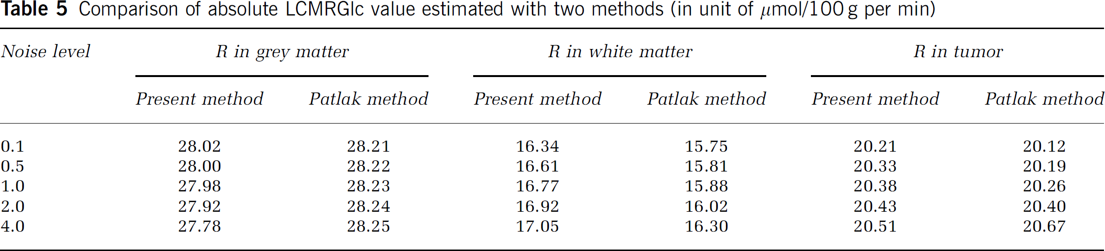
Both measurements of the constant parameter LC and R_g are quite invasive and require other independent experiments. When calculating absolute LCMRGlc value derived from Patlak (or other methods using input function) and the present method, the universality of these constant parameters for the population is assumed. Generally speaking, this assumption is valid for healthy population. There may be some reasons to consider that the fluctuation of LC among the population is slightly lower than the fluctuation of R_g, but the measurement of LC also needs the measurement of R_g (Huang et al, 1980; Hasselbalch et al, 1998). Therefore it is difficult to say that the deviation of LC value is lower than the deviation of R_g value. In fact, the relative error of R_g shown in Hasselbalch et al (1998) is approximately 18%, but the relative error of LC is slightly greater than this value. The constant c_p is required in equation (13), which introduces another uncertainty to LCMRGlc, but equation (14) does not. From this point, the accuracy of LCMRGlc derived from equation (14) is not worse than that derived from equation (13). Because we can use only equation (14) to calculate absolute LCMRGlc with present method, to avoid the difference between using equations (13) and (14) in comparison of absolute values of LCMRGlc with the present method and the Patlak method, the absolute LCMRGlcs in grey matter, white matter, and tumor were calculated using equation (14) and are shown in Table 5. Here R_g is taken as 23 μmol/100 g per min (Hasselbalch et al, 1998). Similar to K/K_g, the relative differences between absolute LCMRGlcs using the two methods are also less than 5%.

Table 5

Comparison of absolute LCMRGlc value estimated with two methods (in unit of μmol/100 g per min)

Noise level	R in grey matter		R in white matter		R in tumor
	Present method	Patlak method	Present method	Patlak method	Present method	Patlak method
0.1	28.02	28.21	16.34	15.75	20.21	20.12
0.5	28.00	28.22	16.61	15.81	20.33	20.19
1.0	27.98	28.23	16.77	15.88	20.38	20.26
2.0	27.92	28.24	16.92	16.02	20.43	20.40
4.0	27.78	28.25	17.05	16.30	20.51	20.67

Similar to LC, the R_g value is quite disperse among different experiments and depends on the measurement methods; the values of R_g in human brain is from 23(Hasselbalch et al, 1998) to 30 μmol/100 g per min (Cohen et al, 1967; Takeshita et al, 1972), and the typical value of LC in human brain is from 0.42 (Phelps et al, 1979; Brooks et al, 1987; Kuwabara et al, 1990) to 0.80 (Hasselbalch et al, 1998). The measured accuracies of both R_g and LC are not very good, therefore the reliability of absolute LCMRGlc value calculated with PET is debatable and all of the known methods cannot yet calculate it very accurately. Usually, the relative value of LCMRGlc already reflects the physiologic or pathologic states quantitively, especially for single subject diagnosis. For the comparison between two different metabolic states of single subject or group study in neural function, the global effect can be removed using scaling or ANCOVA model (Kiebel and Homes, 2004). Adding these constants at present is not necessary. For those situations requiring absolute LCMRGlc value, we may add these constants, but we have to consider this discrepancy. Of course, absolute LCMRGlc value is very important, and how to measure this value noninvasively and accurately in humans requires further studies.

Another important factor to be discussed is the standardized uptake value. It is an index widely used in clinical FDG studies and diagnoses without requiring blood samples. The validity of standardized uptake value depends mainly on two important assumptions and approximations: one is that at the large time T (e.g., more than 45 mins after injection), free FDG is a small fraction of the total radioactivity in tissue and can be neglected; another is that the integral of the PTAC curve is proportional to the injected dose and inversely proportional to body weight or body surface area (Huang, 2000). However, these two assumptions are not always valid. Specially in regarding the progression of disease, standardized uptake value and net FDG clearance estimated with Patlak method give opposite conclusions for some patients. The discrepancies between these two indices are mainly affected by these two assumptions (Freedman et al, 2003). In addition, the recovery coefficient and partial volume effects still exist and they are hardly solved in calculating standardized uptake value (Keyes, 1995; Huang, 2000). Therefore its reliability is still somewhat controversial (Keyes, 1995; Huang, 2000), and its application as a quantitative index should be discouraged (Keyes, 1995). However like Patlak method (the gold standard), the present method is not limited with these factors.

This simulation study shows that the present method is a very consistent one and a good approximation to the Patlak method. This method does not need any information on input function nor requires arterial blood or corrections for the spillover and partial volume when using image-derived input function. Using this method, calculation is simple and easy to perform voxel by voxel, therefore it can be widely used to generate quantified LCMRGlc image not only in laboratory studies but also in clinical application instead of using standard uptake value.