Noninvasive Quantification of rCBF Using Positron Emission Tomography

Abstract

This study proposes a new method for the pixel-by-pixel quantification of regional CBF (rCBF) with positron emission tomography and H₂¹⁵O by using a reference tissue region. No arterial blood is required. Simulation studies revealed that the calculation of rCBF was fairly stable provided that the frame time was relatively short compared with total scan time. In practice, calculated CBF images correlated significantly with those obtained with the dynamic/integral method. Because the method accurately detects changes in CBF, it is particularly suitable for brain activation studies.

Several methods for the measurement of regional CBF (rCBF) using H₂¹⁵O and positron emission tomography (PET) have been described. These include steady-state (Frackowiak et al., 1980), weighted integration (Huang et al., 1982, 1983; Alpert et al., 1984), autoradiographic (Raichle et al., 1983; Kanno et al., 1984), buildup (Lammertsma et al., 1989), and dynamic/integral techniques (Lammertsma et al., 1990). These methods require arterial blood sampling to obtain absolute blood flow values. To measure the time course of the radioactivity concentration in arterial blood accurately, an external detection device is required. However, this measurement should take into account delay and dispersion of the measured blood curve relative to the brain data (Iida et al., 1986). The total amount of blood withdrawn, which can amount to 100–200 ml for a study of several runs, is not small. The present study proposes a new numerical solution for the calculation of rCBF. The method uses time–activity curves of two different brain regions and has the following characteristics:

• The method is noninvasive, requiring no arterial input function and, hence, no corrections for dispersion and time delay are required. More importantly, no arterial cannulation is needed.

• The method produces pixel-by-pixel, functional images of rCBF with short calculation times.

• The calculations proceed automatically without operator's intervention.

The results of simulation and PET studies are presented as well as the theory. The present technique is related to the technique developed by Mejia et al. (1994), which corrects the nonlinearity of CBF and produces the relative CBF image.

THEORY

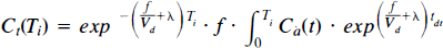
The method is based on the single compartment model originally developed by Kety (1951), in which the differential equation between tissue radioactivity concentration and arterial input function can be described as follows:

$\frac{d{C}_t(t)}{dt}=f{C}_a(t)-\frac{f}{V_d}{C}_t(t)$

(1)

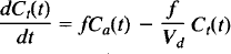
where C_t(t) and C_a(t) reflect the tissue radioactive concentration values at time t in the brain and arterial blood, respectively, f is the rCBF, and V_d is the distribution volume of water. Both C_t(t) and C_a(t) are decay corrected.

Choosing any two regions called Regions 1 and 2 in the brain, Eq. 1 can be described for both regions as:

$\frac{d{C}_{t1}(t)}{dt}=f_1{C}_a(t)-\frac{f_1}{V_{d1}}{C}_{t1}(t)$

(2)

$\frac{d{C}_{t2}(t)}{dt}=f_2{C}_a(t)-\frac{f_2}{V_{d2}}{C}_{t2}(t)$

(3)

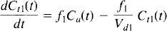
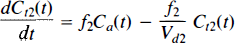
where the subscripts denote the respective regions. It is assumed that the input functions C_a(t) is the same for all brain regions.

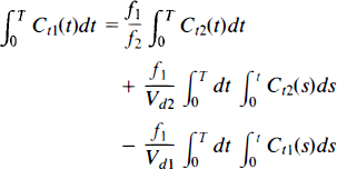
Integrating both Eqs. 2 and 3 twice from time 0 to T results in

$\begin{array}{rl}{\int }_0^T{C}_{t1}(t)dt=& f_1{\int }_0^{T}dt{\int }_0^t{C}_a(s)ds\\ & -\frac{f_1}{V_{d1}}{\int }_0^{T}dt{\int }_0^t{C}_{t1}(s)ds\end{array}$

(4)

$\begin{array}{rl}{\int }_0^T{C}_{t2}(t)dt=& f_2{\int }_0^{T}dt{\int }_0^t{C}_a(s)ds\\ & -\frac{f_2}{V_{d2}}{\int }_0^{T}dt{\int }_0^t{C}_{t2}(s)ds\end{array}$

(5)

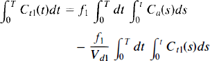
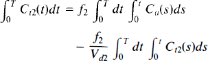
where T is the time of the last frame for PET scan. The arterial input function C_a can be eliminaed from Eqs. 4 and 5:

$\begin{array}{rl}{\int }_0^T{C}_{t1}(t)dt=& \frac{f_1}{f_2}{\int }_0^T{C}_{t2}(t)dt\\ & +\frac{f_1}{V_{d2}}{\int }_0^{T}dt{\int }_0^t{C}_{t2}(s)ds\\ & -\frac{f_1}{V_{d1}}{\int }_0^{T}dt{\int }_0^t{C}_{t1}(s)ds\end{array}$

(6)

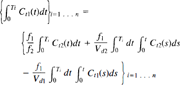
For a PET scan with n frames, n data sets for Eq. 6 are obtained:

$\begin{array}{rl}& {\{{\int }_0^{Ti}{C}_{t1}(t)dt\}}_{i=1\dots n}=\\ & \{\frac{f_1}{f_2}{\int }_0^{T_i}{C}_{t2}(t)+\frac{f_1}{V_{d2}}{\int }_0^{T_i}dt{\int }_0^t{C}_{t2}(s)ds\\ & {-\frac{f_1}{V_{d1}}{\int }_0^{T_i}dt{\int }_0^t{C}_{t1}(s)ds\}}_{i=1\dots n}\end{array}$

(7)

To calculate CBF on a pixel-by-pixel basis, a two-step computational strategy was developed. In the first step, the whole brain was defined as Region 1 and all pixels within 10% of the maximum counts as Region 2. The integrated image from time zero to T was created and made the histogram for distribution of pixel counts. Pixels within 10% of the maximum counts were defined as the pixels being in the higher 10% of the histogram. Using the corresponding time–activity curves, whole-brain CBF (f₁) and distribution volume of water (V_a1), together with f₂ for Region 2 were fitted using standard non-linear regression techniques. To reduce the number of parameters, the distribution volume of water for Region 2 (V_d2) was fixed to 0.86 ml/ml (Lammertsma et al., 1992).

In the second step, f₁ and V_d1 were fixed to these fitted values and each pixel was, in turn, used for Region 2. For each pixel f₂ was calculated according to

$f_2=\frac{{\int }_0^T{C}_{t2}(t)dt}{\begin{array}{c}\frac{1}{f_1}{\int }_0^T{C}_{t1}(t)dt+\frac{1}{V_{d1}}{\int }_0^{T}dt{\int }_0^t{C}_{t1}(s)ds-\\ \frac{1}{V_{d2}}{\int }_0^{T}dt{\int }_0^t{C}_{t2}(s)ds\end{array}}$

(8)

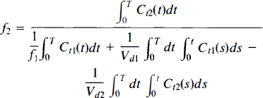
which can be derived from Eq. 6. In this calculation, V_d2 was also fixed to 0.86 ml/ml.

MATERIAL AND METHODS

Simulations

To evaluate the accuracy and limitations of the method, computer simulations were performed to examine (a) the effects of the total study duration, (b) the effects of single-frame duration, (c) the effects of noise, (d) the effects of flow in Region 2, (e) the effects of an incorrect assumed distribution volume (V_d), and (f) the effects of heterogeneity of gray and white matter.

Using the following equation, tissue time–activity curves [C_t(T_i)] of Region 1 and Region 2 were generated:

$C_t(T_i)=ex{p}^{-(\frac{f}{V_d}+\lambda )T_i}\cdot f\cdot {\int }_0^{T_i}{C}_a(t)\cdot (t)\cdot ex{p}^{(\frac{f}{V_d}+\lambda )t_{dt}}$

(9)

where C_a(t) is an arbitrary measured arterial input function. In these simulations, two typical input curves were used, one for a 2-min inhalation of C¹⁵O₂ (Input 1) and one of a 1-min infusion of H₂¹⁵O (Input 2) (Fig. 1).

FIG. 1.

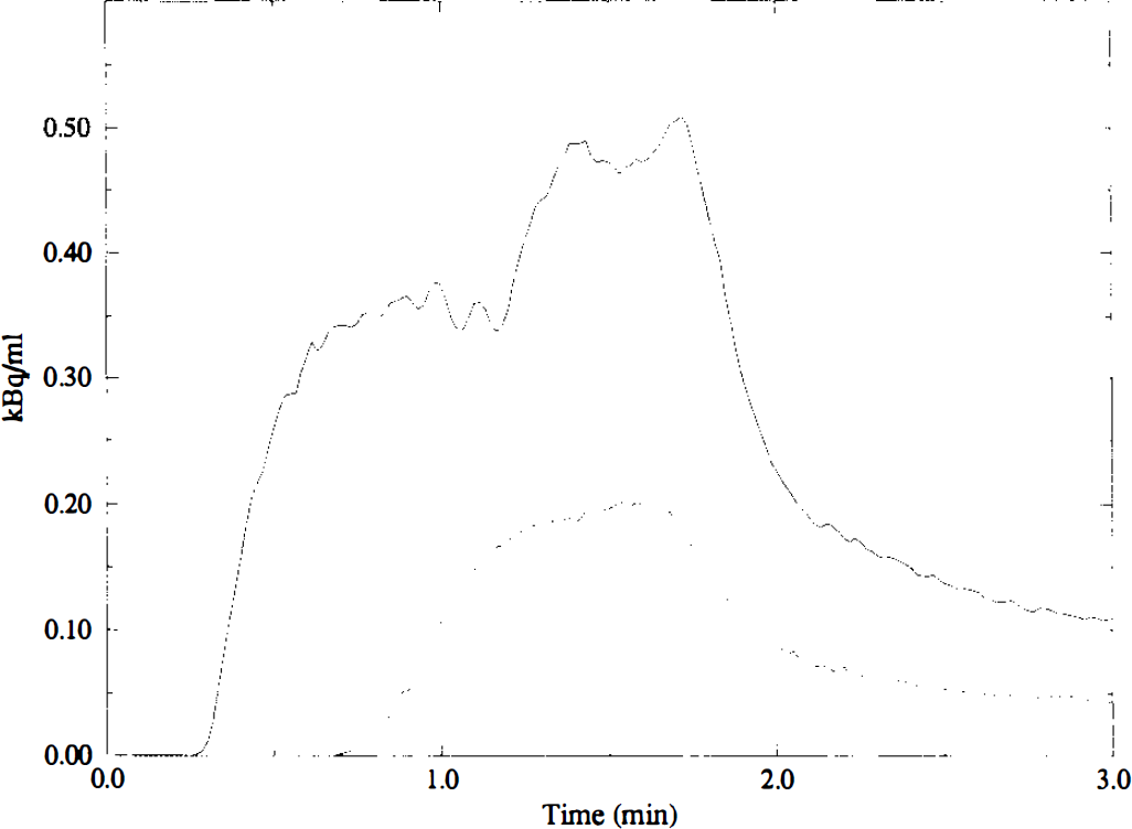
Input functions of Input 1 (2-min C¹⁵O₂ inhalation study, solid line) and Input 2 (1 min H₂¹⁵O infusion study, dotted line). These curves were used in the simulation studies. The tissue response curves for Regions 1 and 2 were calculated with these input functions.

In each simulation, flows of Regions 1 and 2 and V_d of Region 1 were estimated using Eq. 7 and standard non-linear regression analysis.

The simulations were carried out on a workstation (SparcStation IPX; Sun Microsystems, Mountain View, CA, U.S.A.).

PET studies

To validate the method, a comparison between the present method and dynamic/integral method (Lammertsma et al., 1990) were carried out with actual PET data. PET studies with C¹⁵O₂ inhalation on 17 normal volunteers (ages: 20–59, mean 40.8 ± 14) were performed. Data were acquired using an ECAT 931-08/12 (CTI, Knoxville, TN, U.S.A.) positron emission tomograph (Spinks et al., 1988).

Before a 2-min dynamic C¹⁵O₂ scan, a transmission scan was performed using external ⁶⁷Ge/⁶⁸Ga ring sources for tissue attenuation correction purposes. Dynamic scans were collected using the following protocol: 1 (background) frame of 30 s, 4 of 5 s, and 16 of 10 s. Subjects inhaled a constant supply of C¹⁵O₂ for 2 min beginning at the start of the second frame. Arterial blood radioactivity was measured using an on-line detection system. Blood was withdrawn continuously through a radial artery cannule at a speed of 5 ml/min using polyethene tubing (length 65 cm from cannula to scintillation crystal) with an internal diameter of 1 mm and a wall thickness of 0.5 mm. For each study, blood withdrawal was started first and scanning commenced when all tubing components were filled with blood. Four minutes after start of scanning, one 2-ml calibration sample was collected through a three-way tap positioned directly behind the BGO scintillator. After the collection of this calibration sample, the whole-blood circuit (including cannula) was flushed with heparinized saline.

All emission scans were reconstructed using a Hanning filter with a cutoff frequency of 0.5 of maximum, which resulted in a spatial resolution of 8.4 × 8.3 × 6.6 mm full width at half-maximum at the center of the field of view (Spinks et al., 1988).

Image processing

The reconstructed dynamic images were transferred to a SparcStation IPX (Sun Microsystems, Mountain View, CA, U.S.A.) for image processing. Whole-brain regions of interest (ROIs) were defined on planes 6–10 of the 15 planes of integrated images, created by summing counts of all frames during the 2-min inhalation period. By projecting these ROIs on the 21 dynamic frames and averaging over the 5 planes, the time–activity curve of the whole brain was generated. This time–activity curve was used for both methods. For the present method, these data were used directly in the process of fitting of Eq. 7. For the dynamic/integral method, this curve was used to determine delay and dispersion of the arterial whole-blood curve (Lammertsma et al., 1990).

A computer program was developed for the pixel-by-pixel calculation of rCBF using the present method. The procedure steps were as follows.

1. To fit for f₁, V_d1,f₂ in Eq. 7 and to calculate rCBF for each pixel using Eq. 8, single and double integrals, i.e., ∫ C_t ∫ ∫ C_t were calculated numerically. Sampling the data without on-line decay correction, data were numerically corrected for decay using the reconstructed images of each frame. The double integration ∫ ∫ C_t for each pixel was calculated numerically using the trapezoidal rule.

2. Pixels within 10% of the highest value in the integrated images were determined and averaged to create the time activity curves in the (Region 2) (C_t2).

3. Using Eq. 7, best estimates for the three parameters f₁ V_d1, f₂ were obtained by fitting.

4. Fixing f₁, and V_d1 to the values obtained in step 3, f₂ was calculated for each pixel using Eq. 8.

Another set of rCBF images was calculated by the dynamic/integral method (Lammertsma et al., 1990) to compare with the present method.

RESULTS

Simulations

An evaluation was made of the effects of total scan time on the calculated rCBF. Sequential tissue data were generated for Regions 1 and 2 using 5-s frames and total study duration up to 300 s. CBF was assumed to be 50 ml/dl/min in Region 1 and 100 ml/dl/min in Region 2 with corresponding V_d values of 0.6 ml/ml and 0.86 ml/ml, respectively (0.6 ml/ml for Region 1 was chosen because of the tissue heterogeneity. It will be examined at the last simulation study). Using these tissue data, f₁, V_d1, and f₂ were estimated. Figure 2 illustrates that CBF of Regions 1 and 2 were generally overestimated, whereas V_d of Region 1 was underestimated when the study time was shortened. However, the estimation of V_d was more stable than that of CBF. Although the general pattern was the same, for Input 1 (C¹⁵O₂ inhalation) a shorter study duration was required than for Input 2 (H₂¹⁵O infusion). For Input 1 the error in f₁ was <5% after only 75 s, whereas for Input 2 a study duration of 110 s was required.

FIG. 2.

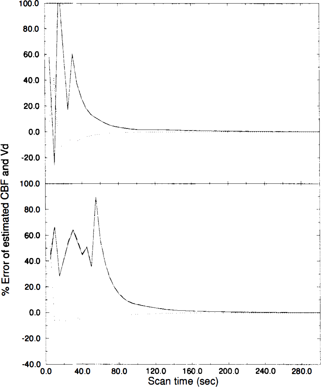
The effects of total study duration on the calculations of rCBF. The upper graph shows the results for Input 1, and the lower graph those for Input 2. Percentage of error in estimated CBF for Region 1 (solid line), estimated V_d for Region 1 (dotted line) and estimated CBF for Region 2 (dashed line) are plotted against study duration with a fixed frame length of 5 s.

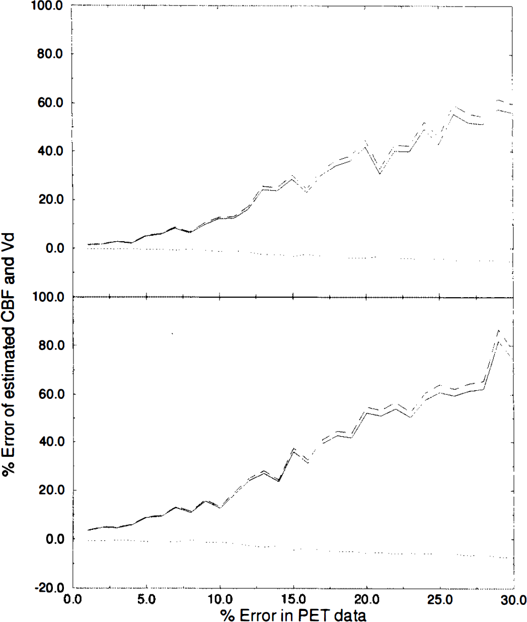
The effects of frame duration are shown in Figure 3. The frame time was varied from 1 to 30 s. Tissue curves for a total scan duration of 120 s were generated for Regions 1 and 2 using the same parameter values as for the previous simulation. As shown in Fig. 3, errors in estimated CBF values increased with increasing frame time. The estimations of V_d1 were more independent of frame time than the estimations of CBF. For Input 2, a stronger influence of frame time was observed. According to these results, a frame length of 9 s was required for Input 1 to reduce the error to <5%, whereas for Input 2 a frame length of 6 s is required.

FIG. 3.

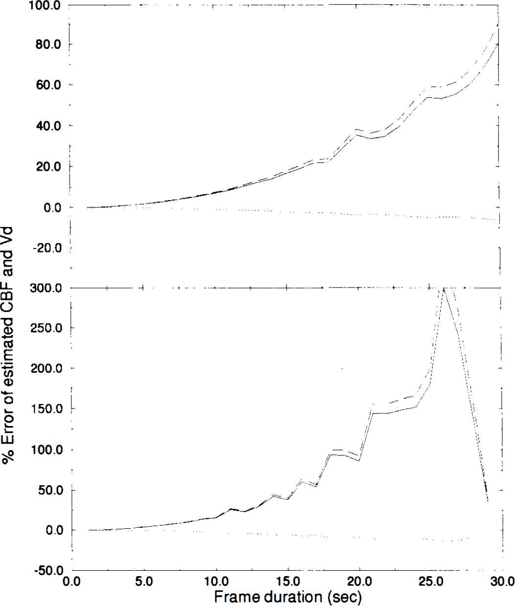
The effects of frame duration on the calculation of rCBF and V_d. The upper graph shows the results for Input 1, and the lower graph those of Input 2. Percentage error in estimated CBF at Region 1 (solid line), estimated V_d for Region 1 (dotted line) and estimated CBF at Region 2 (dashed line) are plotted as a function of frame duration.

Random noise with a variance of up to 30% was added to every point of the tissue curves for Regions 1 (flow: 50 ml/dl/min, V_d: 0.6 ml/ml) and 2 (flow: 100 ml/dl/min, V_d: 0.86 ml/ml). The rCBF for Regions 1 and 2 and V_d for Region 1 were calculated with 5-s frame, 120-s study duration. These simulations were carried out 100 times with different random noise and the data obtained were averaged. Higher noise levels produced larger errors in the calculated values as shown in Fig. 4. Calculations of V_dl were more stable with respect to noise in the PET data than the calculations of CBF. Again, Input 1 resulted in smaller errors than Input 2.

FIG. 4.

Simulation of errors due to statistical noise. Random noise with a variance of 1–30% was added to tissue counts. The upper graph shows the results for Input 1, and the lower graph for Input 2. Percentage errors of estimated CBF for Region 1 (solid line), estimated V_d for Region 1 (dotted line), and estimated CBF for Region 2 (dashed line) are plotted against noise level.

To evaluate the relationship between flow at Region I and flow at Region 2, tissue data were generated for Region I (flow 50 ml/dl/min, V_d: 0.6 ml/ml) and Region 2 (V_d: 0.86 ml/ml). Flow of Region 2 was varied from 60 to 120 ml/dl/min. Figure 5 indicates that as flow of Region 2 approached that of Region 1, there was a slight increase in the estimation of CBF. Tendencies for estimated flow and V_d between Input 1 and Input 2 are similar for Input 1 and Input 2.

FIG. 5.

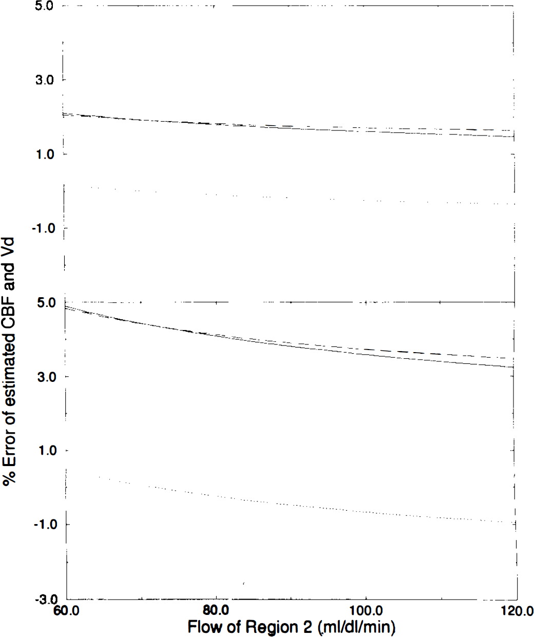
The effects of rCBF of Region 2. The upper graph shows the results for Input 1, and the lower graph those for Input 2. Percentage error of estimated CBF for Region 1 (solid line), estimated V_d for Region 1 (dotted line), and estimated CBF for Region 2 (dashed line) are plotted against flow value of Region 2.

The effect of the fixed distribution volume in Region 2 is illustrated in Fig. 6. Tissue data for Region 2 were generated with a flow of 100 ml/dl/min and a V_d ranging from 0.69 to 1.03 ml/ml. Tissue data for Region 1 were the same as before. Frame and study duration were fixed at 5 and 120 s, respectively. V_d for Region 2 was fixed to 0.86 ml/ml in the fitting process. Figure 6 illustrates the errors obtained due to this incorrect assumed distribution volume. If actual V_d was smaller than 0.86 ml/ml, estimated flows and V_dl were overestimated. The opposite was true for larger actual V_ds, although the effect of a smaller V_d was more pronounced in absolute terms.

FIG. 6.

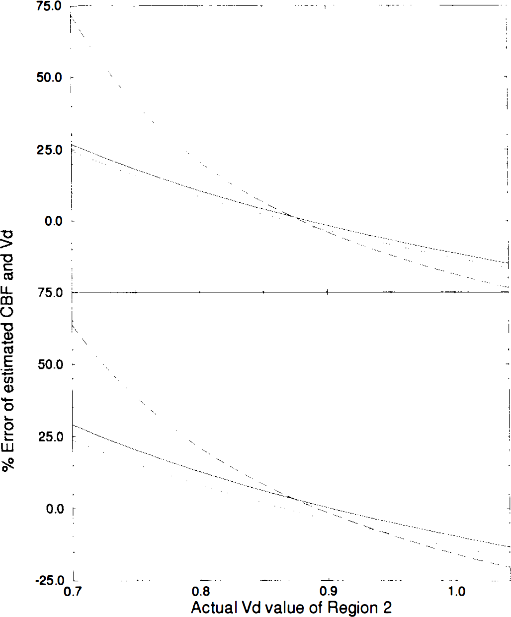
Errors due to incorrect distribution volume. The upper graph shows the results for Input 1, and the lower graph those for Input 2. Percentage error of estimated CBF for Region 1 (solid line), estimated V_d for Region 1 (dotted line) and estimated CBF for Region 2 (dashed line) are plotted against actual distribution volume value of Region 2.

To assess the effects of tissue heterogeneity, tissue data of gray matter (CBF = 80 ml/dl/min; V_d = 1.02 ml/ml) and white matter (CBF = 20 ml/dl/min; V_d = 0.88 ml/ml) were generated. The tissue time–activity curves of Region 1 with different fractions of gray and white matter were created using weighted averages of the stimulated gray and white matter curves. The tissue data of Region 2 were also generated as CBF = 100 ml/dl/min; V_d = 0.86 ml/ml). Study and frame duration were fixed to 120 and 5 s, respectively. Figure 7 demonstrates the effect of tissue heterogeneity on estimated values of flows and V_d1. It can be seen that all fitted values were underestimated. Estimations of flows were affected more by tissue heterogeneity than by V _d .

FIG. 7.

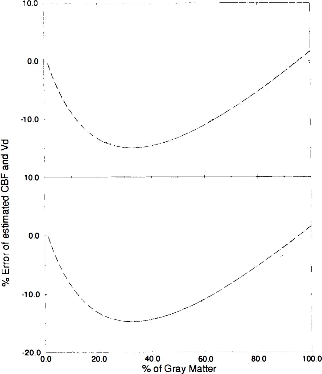
The effects of tissue heterogeneity in Region 1 for different fractions of gray matter on estimations of flow and distribution volume. The upper graph shows the results for Input 1, and the lower graph those for Input 2. Percentage error of estimated CBF for Region 1 (solid line) estimated V_d for Region 1 (dotted line) and estimated CBF for Region 2 (dashed line) are plotted against percentage of gray matter.

PET studies

To validate the present method, it was compared with the dynamic/integral method (Lammertsma et al., 1990) on the same subjects.

Figure 8 presents examples of functional CBF images obtained with both methods together with the corresponding summed images. The images obtained with the present method were very similar to those obtained with the dynamic/integral method, and the contrast of both sets of images was enhanced compared with the summed images.

FIG. 8.

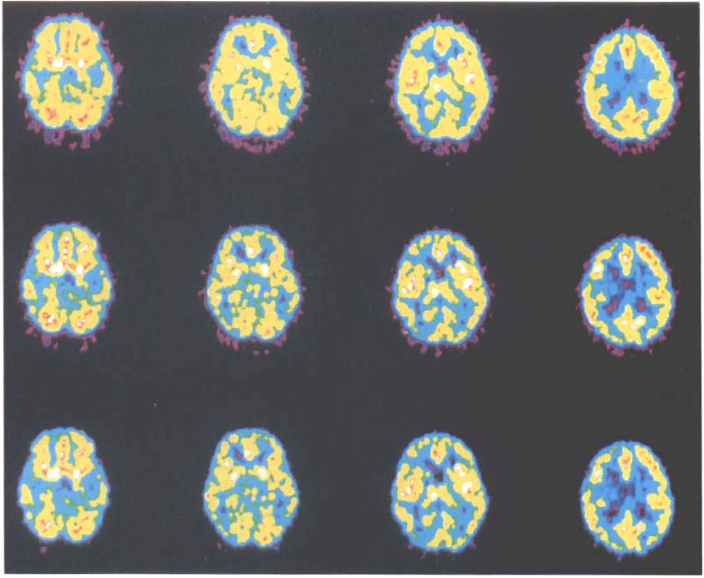
First row depicts summed images (from 2 to 15 frames) of 2-min C¹⁵O₂ inhalation study of normal volunteer. Second row is functional rCBF images calculated by the dynamic/integral method. Third row depicts functional rCBF images calculated by the present method.

For each subject, the images obtained with both methods were compared by plotting rCBF values for regions of 4 × 4 pixels in all planes against each other. One example of such a plot is shown in Fig. 9. Regression curves and correlation coefficient were calculated for all studies and are shown in Table 1. The mean value was calculated by averaging over all individual pixels in all slices. The mean value was slightly low because some pixels were outside the brain. Figure 10 shows the mean CBF values calculated by both methods for all subjects. To get rid of pixels outside of the brain, the transmission images were used for masking the brain field. The correlation coefficient was 0.749, with a significant correlation between two methods (paired t test, p < 0.0005).

TABLE 1.

Comparison of two methods

Run no.	Mean a	Mean b	Corr. coef.	Slope	Intercept
p1414	26.8	27.7	1.00	1.04	−0.119
p1474	28.7	26.3	1.00	0.909	0.167
p1597	24.9	24.8	1.00	0.985	0.0061
p1634	29.3	28.3	1.00	0.958	0.275
p1639	25.7	26.7	1.00	1.05	−0.128
p1644	36.7	28.0	1.00	0.745	0.659
p1657	33.1	27.2	1.00	0.808	0.470
p1672	26.9	30.9	1.00	1.16	−0.384
p1770	23.4	25.2	1.00	1.08	−0.172
p1803	22.5	22.8	1.00	1.01	−0.0867
p1831	37.8	33.0	1.00	0.861	0.449
p1852	24.5	25.8	1.00	1.06	−0.108
p1865	25.2	25.0	1.00	0.990	0.0144
p1949	27.7	26.9	1.00	0.969	0.0308
p2018	35.3	35.4	1.00	1.00	−0.0098
p2037	33.1	34.8	1.00	1.06	−0.159
p2122	33.4	29.5	1.00	0.875	0.319
Average	29.1	28.1	1.00	0.974	0.0720
SD	4.8	3.6	1 × 10−4	0.107	0.277

a

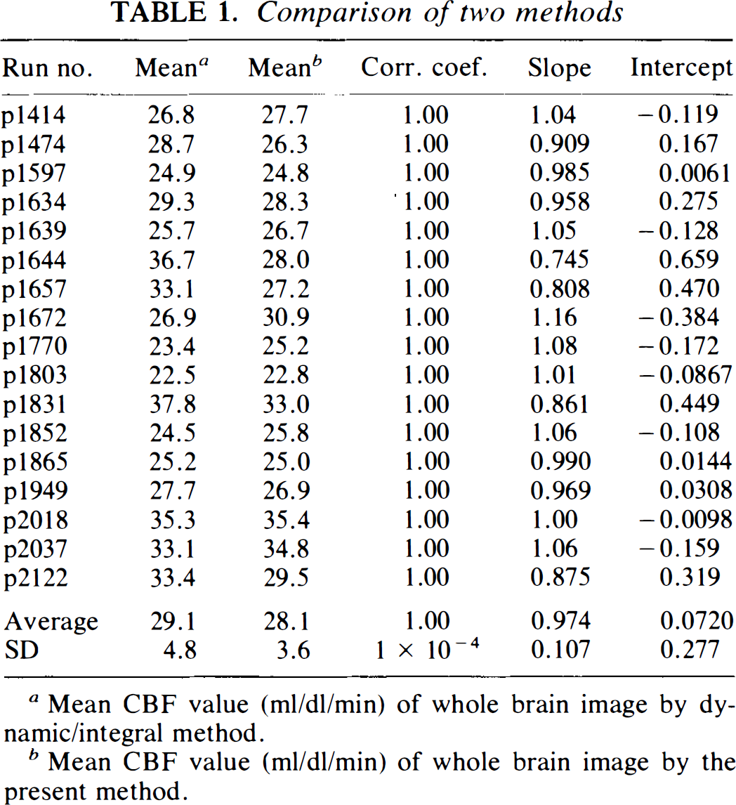
Mean CBF value (ml/dl/min) of whole brain image by dynamic/integral method.

b

Mean CBF value (ml/dl/min) of whole brain image by the present method.

FIG. 9.

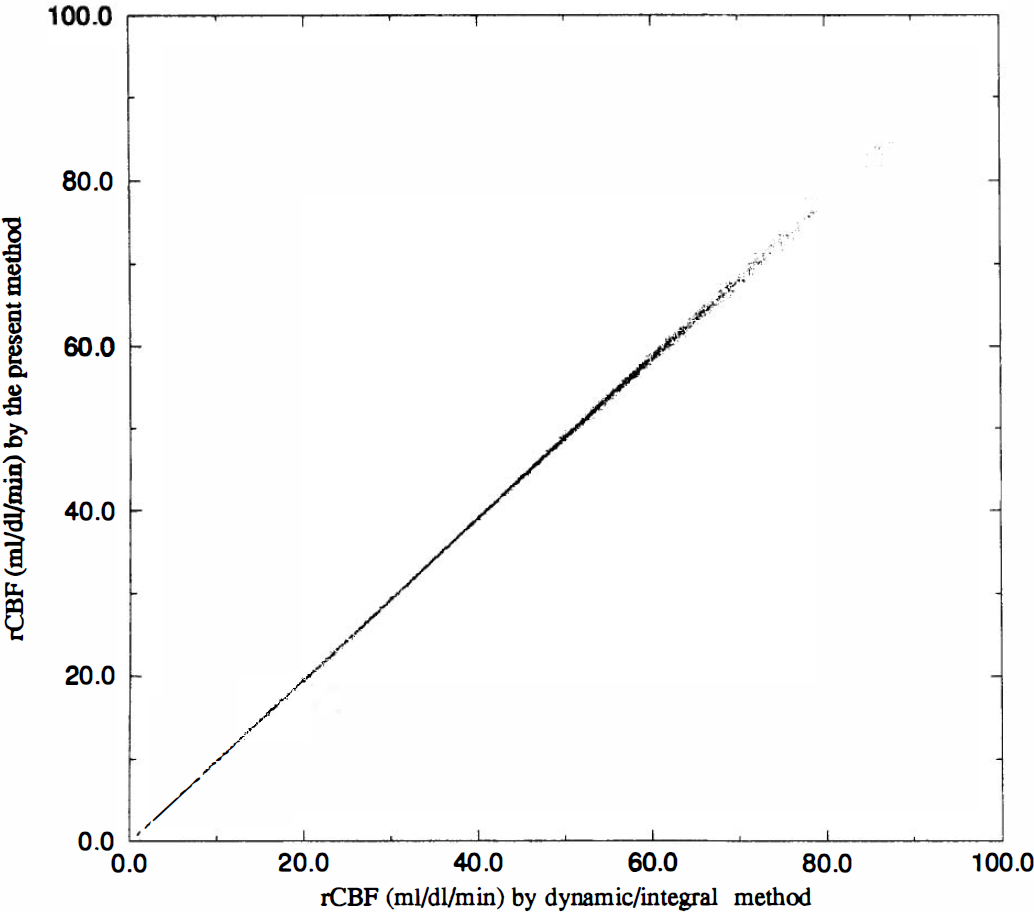
Comparison of rCBF values calculated by the dynamic/integral method (abscissa) and the present method (ordinate). Each plotted point represents 4 × 4 pixels.

FIG. 10.

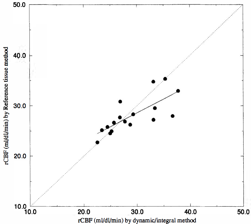
Comparisons of mean rCBF values of 17 subjects calculated by the dynamic/integral method (abscissa) and the present method (ordinate) with a regression curve. The dotted line is the line of identity.

DISCUSSION

Once the feasibility of mapping human brain function with PET and H₂¹⁵O was established, numerous research protocols were developed. However, because PET measurements are relatively long, the state of attention relative to habituation has become a point of concern. The subject's psychological state is often disturbed. In particularly, the presence of an arterial cannula can be a source of unwanted stimulation. Therefore, often activation studies with PET are carried out without arterial sampling. However, this procedure cannot give absolute flow values before and after stimulation. The present noninvasive technique was developed to provide quantitative functional CBF pixel-by-pixel maps without arterial sampling. This technique calculates rCBF at two regions simultaneously, assuming the input function to both regions to be the same and difference in arrival to be relatively small (Iida et al., 1988).

The main weakness of the proposed method is that it relies on PET data of two regions simultaneously. Inaccuracies in both regions will affect the final result. In particular, for Region 2 V_d is assumed to be 0.86 ml/ml. From Figure 6 it follows that potentially large errors may result if the actual value of V_d is very different. However, a large variation in V_d for this region is unlikely. Lammertsma et al. (1992) found for a similar region a coefficient of variation was <5% (n = 12). If the CBF value for Region 2 is too close to that for Region 1, the error sensitivity will increase (Figure 5). Again, by choosing a whole brain ROI and an ROI containing only the maximum 10% of the pixel values, this situation is unlikely in practice. The present method is also affected by tissue heterogeneity. It is interest to note, however, that in contrast to the dynamic/integral method (Lammertsma et al., 1990), in the present method there was no difference in effect of tissue heterogeneity between flow and V_d (Fig. 7). The model that uses fixed V_d for Region 1 had been applied to calculate flow of Region 1 in Eq. 6, and the results obtained were not as good as in the present method because of the tissue heterogeneity. In the current implementation, the whole brain was used for Region 1 and all pixels that were within 10% of the maximum integrated count for Region 2. Further studies will be required to optimize the selection of Regions 1 and 2.

According to the results shown in Figs. 2 and 3, both a too-short total study duration or a too-long frame time resulted in significant errors, probably due to numerical errors related to integration over discrete data points. There is the alternative method of integration to solve Eq. 6, namely, integrating over each of the n scan frames rather than integrating from 0 time to the end of the nth scan frame. Since the early frames after injection of ¹⁵O may contain errors due to low counts of the PET detector, the integration was carried out from 0 time to the end of the nth scan frame. To reduce such numerical errors, it is desirable to select shorter frame times and a longer total study duration. However, as shown in Fig. 5, noise propagation errors should also be taken into account. These errors become more pronounced for shorter time frames. Further studies will be required to select the optimal frame duration, taking into account the two effects already mentioned.

The simulation studies that are shown in this article only evaluate the relationship between Region 1 and Region 2. In practice, one is more interested in the flows in individual pixels obtained by Eq. 8 rather than the values obtained for flow in these reference regions. As shown in Table 1 and Fig. 9, the correlation coefficient is fairly good (most are 1) between our method and the dynamic/integral method, which suggests that the process to calculate each pixel's flow associated with Eq. 8 is equivalent to the process of the dynamic/integral method. The simulation studies which evaluate Eq. 8 and the relative relationship between flows in Region 1 and Region 2 have been carried out by Mejia et al. (1994).

The main problem of the present method is shown in Fig. 11. This error surface was created as follows.

FIG. 11.

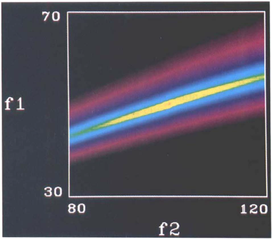
Error surface image generated by simulation data.

Using simulated tissue data (frame and total study duration were 5 and 120 s, respectively) of Region I (CBF = 50 ml/ml/min; V_d = 0.6 ml/ml) and Region 2 (CBF = 100 ml/ml/min; V_d = 0.86 ml/ml), sums of squares of the right side of Eq. 7 were calculated for different combinations of f₁ and f₂. f₁ was varied from 30 to 70 dl/ml/min and/₂ from 80 to 120 dl/ml/min. Results were plotted as an image with highest pixel value for the lowest sums of squares. This error surface image demonstrates that, although there is a solution at the center (f₁ = 50 dl/ml/min; f₂ = 100 dl/ml/min, the brightest point in the image), the error surface broadens from low-flow to high-flow area, that is, this solution is very near to singular. The error surface is somewhat shallow when noise is added within the actual PET data; local minima could give rise to solutions that are dependent on the starting values in the fitting routine. The disagreement between the two methods in the high-flow study in Fig. 10 may represent this problem. It is important that the scanning protocol be optimized (see previous discussion) to obtain better-defined solutions. In addition to frame duration and selection of reference region, attention should be paid to the input function. From the simulation it follows that a 2-min administration period performs better than a 1-min period. Again, this needs to be further optimized.

Despite the problems already discussed, in practice, good results were obtained. In particular, the intra- and inter-subject correlations with the dynamic/integral method (Figs. 9 and 10) are promising and warrant further investigation of the method.

The major advantage of the proposed new technique is that it does not require blood sampling. In addition, the calculation is relatively simple and can generate rCBF images quickly after completion of the PET scans.