From Homogeneous to Fractal Normal and Tumorous Microvascular Networks in the Brain

Abstract

We studied normal and tumorous three-dimensional (3D) microvascular networks in primate and rat brain. Tissues were prepared following a new preparation technique intended for high-resolution synchrotron tomography of microvascular networks. The resulting 3D images with a spatial resolution of less than the minimum capillary diameter permit a complete description of the entire vascular network for volumes as large as tens of cubic millimeters. The structural properties of the vascular networks were investigated by several multiscale methods such as fractal and power-spectrum analysis. These investigations gave a new coherent picture of normal and pathological complex vascular structures. They showed that normal cortical vascular networks have scale-invariant fractal properties on a small scale from 1.4 μm up to 40 to 65 μm. Above this threshold, vascular networks can be considered as homogeneous. Tumor vascular networks show similar characteristics, but the validity range of the fractal regime extend to much larger spatial dimensions. These 3D results shed new light on previous two dimensional analyses giving for the first time a direct measurement of vascular modules associated with vessel-tissue surface exchange.

Introduction

Cortical microvascular organization is an important biological issue for a broad range of fundamental and clinical subjects such as normal and pathologic vascular development (Hobbs et al, 1998; Yuan et al, 1996), functional imaging interpretation (Malonek and Grinvald, 1996), micro-circulatory modeling (Lichtenbeld et al, 1996), and therapeutic strategies (Jain, 2005). As microvascular networks are extremely complicated structures, some relevant structural parameters are needed to describe angiogenic maturation or to define malignancy criteria. Previous studies have used simple parameters such as vascular density in normal cortical tissues and fractal dimension in retinal (Family et al, 1989), pial (Hermán et al, 2001) or tumor (Gazit et al, 1995, 1997; Baish and Jain, 2000) vascular networks. These analyses have pointed out the interest of fractal analysis to address taxonomic issues for either healthy (Hermán et al, 2001) or pathologic (Gazit et al, 1995; Baish and Jain, 2000) vascular networks. In some of these previous investigations, cancer vascular networks were found to be fractal, whereas normal vascular networks were not (Gazit et al, 1995; Baish and Jain, 2000). Nevertheless, some other investigations of two-dimensional (2D) vascular networks in normal tissues have also found multiscaled properties for such healthy structures (Family et al, 1989; Hermán et al, 2001). The analysis of the spatial multiscaled characteristics of vascular structures has been recently completed by the investigation of their temporal functional variations, averaged over a three-dimensional (3D) volume. Different investigations of the cerebral blood flow (CBF) in human cerebral cortex using near infrared spectroscopy have observed multiscaled self-affine temporal fluctuations (Eke et al, 2002, 2005; Eke and Delpy 1999). These measurements have permitted the estimation of the dynamical fractal exponent associated with the power law behavior of the power spectra of CBF temporal fluctuations. These parameters have shown significant statistical differences concerning age and gender (Eke et al, 2005), and thus they provide interesting insights into human brain hemodynamics. These very interesting observations now raise new questions concerning the relationship between spatial and temporal multiscaled characteristics of brain microvascular networks, as pointed out by Eke et al (2005).

The quality of multiscaled analysis can nevertheless suffer from a lack of spatial resolution (Chung and Chung, 2001; Baish and Jain, 2001). Moreover, when considering spatial multiscaled properties, most of the previous studies restricted their investigation to 2D analysis. The reason for this restriction was two-fold: either the vascular network under study was on a surface (retinal or pial vascular networks) or technical limitations prevented the analysis of full 3D networks. Most previous studies have used conventional microscopy techniques in which the illuminating radiation has a finite penetration depth, so that the investigation of tissue volume is limited to within a depth of a few hundreds of micrometers (Polimeni et al, 2005). More recent techniques, such as multiphotonic (Brown et al, 2001; Chaigneau et al, 2003) and intra-vital microscopy (Jain et al, 2002) give promising evidence that coupled vascular and neuronal in vivo information could be obtained at the capillary scale. These new techniques are nevertheless also restricted to a rather limited region of interest. High-resolution synchrotron tomography has recently been proposed for more complete 3D imaging of microvascular networks (Plouraboué et al, 2004). The present paper uses this method to statistically compare normal and tumor vascular structural multiscale organization from the micrometer to the millimeter scale, in 3D. Using this new technique, we re-address the question of how normal and tumorous vascular structures differ. The investigation proposed in this paper resolves the apparent contradiction of previous studies for which normal vascular networks have been found to be either fractal or not. Moreover it gives some new insight into the 3D organization of the cerebral gray matter, thus allowing a quantitative estimation of the ‘vascular modules.’ This concept is important because such modules might be linked to already well-identified neuronal functional modules (Devor et al, 2005). Only indirect estimation of the spatial extent of these modules has been proposed so far from submillimeter-scale functional imaging observations (Turner, 2002). This paper proposes a direct identification of the ‘vascular modules' through the investigation of the multiscale organization of microvascular networks on the micrometer scale.

Materials and Methods

The vascular structure of the brain cortical gray matter of both adult rats and primates was studied. The first species was chosen for tumor implantation because a well-established protocol already existed (Weizsaecker et al, 1981; Van der Sanden et al, 2000). Moreover, the 9L gliosarcoma has been the most widely used of all the rat brain models (Weizsaecker et al, 1981). The monkey cortex was chosen as a good model of the human cortex.

Cell Line

The 9L gliosarcoma cell line used was originally established by Benda et al (1971) by the intravenous injection of N-methylnitrosourea for 26 weeks to CD Fischer rats. Cells were grown as monolayers with Dulbecco's modified Eagle's medium (DMEM) (Gibco-Invitrogen-France, Cergy-Pontoise, France) without sodium pyruvate (with 4,5 mg/L of glucose and pyridoxine HCL, supplemented with 10% fetal calf serum and 0.2% penicillin/streptomycin. They were incubated at 37°C in a mixture of air/CO₂ (95/5%).

Tumor Implantation

The male Fischer 344 rats (180 to 280 g, Charles River, L'Arbresle, France) were anesthetized by a 5% isoflurane inhalation followed by an intraperitoneal injection of 400 mg/kg of chloral hydrate. The rats were placed on a stereotactic head holder (model 900, David Kopf Instruments, Tujunga, USA) after anesthesia. Before injection into the brain, 10⁴ cells were suspended into 1 μL of DMEM with antibiotics (1%). The cell suspension was manually injected according to a method derived from (Kobayashi et al, 1980) using a 1 μL Hamilton syringe through a burr hole (0.8 mm diameter) in the right caudate nucleus (7.5 mm anterior to the zero earbars, 3.5 mm lateral to the midline, 3 mm depth from the dura). The syringe was gently removed 1 min after the injection. The burr hole was plugged with dental cement and the scalp was sutured. The operative field was cleaned with povidone-iodine before closure of the scalp incision. The rats were temporarily housed in a 27°C thermostated incubator, to minimize the surgical shock. The duration of the housing at 27°C depended on the duration of the anesthesia. The rat stayed in the incubator for about 2 h, from the time it was anesthetized, until it was able to stand up and walk. It was then sent back to the rodent housing area, where food and water were provided ad libitum.

The tumors were implanted according to a standard in-house procedure, also used for other experiments. With this procedure it is known that

• (i) the survival of rats affected by these tumors is equal to 19.75 ±1.69 Days (D) (n = 25 rats).

• (ii) the average diameter of the largest section of the tumor is 5 mm at D13 to D14 in this tumor model.

• (iii) There is no evidence of a necrotic area at D14, although a pseudo-palisading pattern (typical of hypoxia) can be seen at these stages. These results obtained on this tumorese model are in agreement with the literature (Dilmanian et al, 2002; Laissue et al, 1998); moreover, they also mimic human glioblastoma. The variability that we have observed on the tumor size presented in this study is 0.9 mm, while the smallest tumor diameter is close to 2 mm.

All procedures related to animal care strictly conformed to the Guidelines of the French Government (licenses 380324/380456 and A3818510002).

Contrast Agent Injection

The injections were performed from D + 12 to D + 16 after implantation. The animals were euthanized by lethal intraperitoneal injection of pentobarbital before contrast agent injection. The same injections were also performed on healthy rats and adult marmoset monkeys (Callithrix jacchus, 350 to 450 g obtained from the CERCO rearing facilities in Toulouse). Details of the tissue preparation protocol can be found in a previous publication (Plouraboué et al, 2004). Briefly, after a surgical step allowing injection of the contrast agent (suspension of barium sulfate solid particles at a concentration of 600 mg/mL), the brain was dissected and fixed in formol 10%. After fixation, samples were cut by means of a cylindrical surgical biopsy punch having an internal diameter of 3 mm.

Tissue Samples

In rats the samples were taken at the tumor injection site (T1 to T4, in four different rats), or in similar sites for two control rats (R1 and R2). In two monkeys, different cortical areas (visual, somato-sensory, somato-motor, temporal cortex) were sampled (M1 to M5). These samples were then dehydrated and included in resin. This procedure induced a 20% to 30% volume shrinkage of the tissue. This volume shrinkage was directly quantified by comparing the apparent diameter of the sample to its original 3 mm. A simple homothetic rule was then applied to transform voxel measurements into physical distances, like those given in Table 1.

Table 1

Quantitative estimates of the structural parameters extracted from fractal and distance map analysis

Sample	Fractal				Fourier			S/V
	D bc	D sb	ℓc BC	ℓcSB	ℓ	v(xy)	v (z)
M 1	1.7±0.1	1.8±0.1	62	84	48	4.9	5.3	5.84
M 2	1.5±0.1	1.55±0.1	53	76	24	4.8	5.6	4.04
M 3	1.55±0.1	1.7±0.1	58	82	64	4.8	5.5	5.13
M 4	1.65±0.1	1.8±0.1	60	64	66	4.9	5.6	3.46
M 5	1.6±0.1	1.75±0.1	50	80	55	4.8	5.6	4.92
R 1	1.7±0.1	1.9±0.1	42	70	48	5.2	5.3	7.24
R 2	1.6±0.1	1.8±0.1	42	82	51	5.0	5.6	5.19
T 1	2.2±0.1	2.4±0.1	88	91	137	4.3	5.2	6.39
T 2	1.9±0.1	1.9±0.1	62	156	121	5.0	5.3	6.25
T 3	2.2±0.1	2.4±0.1	106	218	113	5	4.5	11.24
T 4	2.±0.1	2.1±0.1	140	184	341	4.5	5.3	6.42

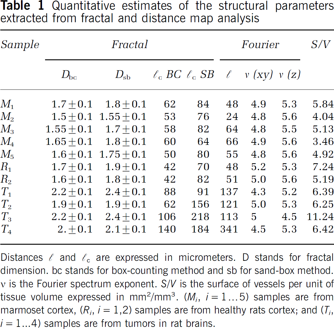
Distances ℓ and ℓ_c are expressed in micrometers. D stands for fractal dimension. bc stands for box-counting method and sb for sand-box method. V is the Fourier spectrum exponent. S/V is the surface of vessels per unit of tissue volume expressed in mm²/mm³. (M_i, i =1…5) samples are from marmoset cortex, (R_i, i = 1,2) samples are from healthy rats cortex; and (T_i, i = 1…4) samples are from tumors in rat brains.

Image Acquisition

After casting in epoxy-resin, the tissue samples had cylindrical shapes approximately 2.5 mm in diameter and tens of millimeters in length. The diameter of the cylinders was increased to 6 mm with an extra epoxy layer for easy and safe handling of the samples. During image acquisition, the cylinder axis was set vertically, approximately parallel to the z axis of rotation. The samples were imaged with a very intense, monochromatic and parallel synchrotron X-ray beam at experimental station ID19 of the European Synchrotron Radiation Facility (ESRF). The absorption imaging mode was chosen to obtain a signal proportional to the local concentration of contrast agent injected into the vascular network. One thousand and two hundred radiographic projections were acquired for each sample, associated with an angle increment of 180/1200. The X-ray energy was set to 20.5 keV and a spatial resolution of 1.4 μm was chosen for the optical system.

The projections were recorded on a 2048 × 2048 pixel CCD camera, resulting in a total field view of 2.8 × 2.8 mm² (see (Plouraboué et al (2004) for more technical details about the imaging procedure). These radiographic projections were processed using the usual filtered back-projection algorithm associated with the inversion of the Radon transformation. The resulting 3D images were re-cast on 256 gray levels for each voxel. The voxel gray level at each point of the image was proportional to the linear attenuation coefficient related to the contrast agent solution. Because of the very high contrast agent concentrations, the resulting image contrast was very good. This allowed the smallest capillary structures to be displayed in both rat and primate cortex.

Image Analysis

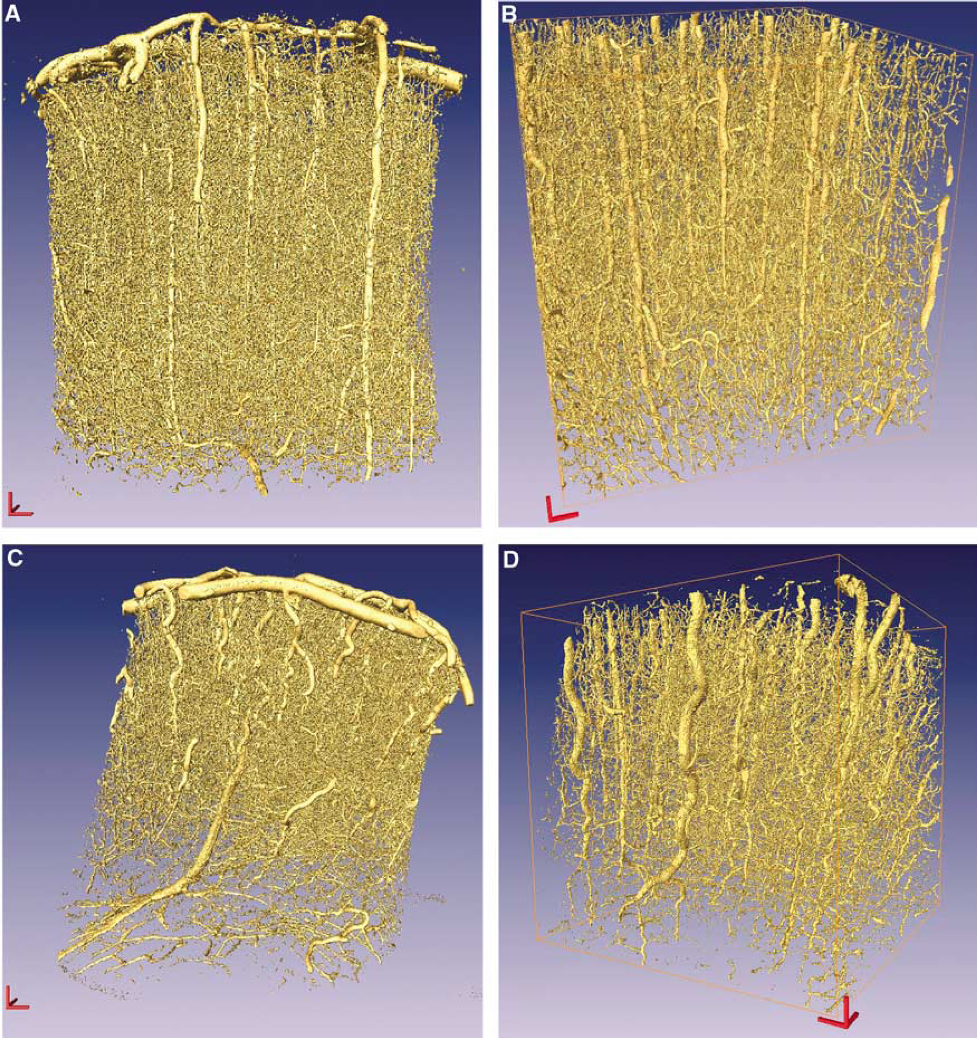
The extremely large data sets generated by the 3D images (each image represents 4 to 5 GB of data), obliged us to develop specific numerical approaches for the image analysis and the data processing. The analysis tools were developed within a native program in C language, so that the successive post-treatment steps could be automated. Images were produced using the commercial software Amira (Mercury, Richmond, TX, USA), which has proven to be a useful tool in this context (Cassot et al, 2006). No prior filtering of the gray-level images has been performed to preserve the information obtained at the capillary scale, as the spatial resolution (1.4 μm) is not so far from the smallest capillary diameter (3 to 5 μm). The first step of the image analysis was the segmentation of the image, transforming 256 gray levels into two distinct levels. We use a standard hysteresis thresholding technique to obtain a first rough binary image. Hysteresis thresholding consists in using two thresholds to select edges. The higher one serves to detect strong edges between ‘white’ voxels to ‘gray’ ones, while the lower covers weak edges that distinguish ‘gray’ voxels from ‘black’ ones. The gray voxels having strong edges are then converted to ‘white’ voxels for they are in their neighborhood. This conversion is applied iteratively until no more change is obtained in the number of voxels in each class. Then the gray voxels are converted to black. Because of the high quality of the image contrast, this binarization procedure was weakly dependent on the chosen values for the thresholds. The resulting binary image was then subjected to conventional 3D erosion-dilation morphological operators processes. Erosion-dilation operators can be visualized as coating or etching the white voxels surfaces so that their surface expands or contracts. These operations enable artificial islands to be eliminated both inside the vessels (black island inside white pixels) and outside the vessels (white island inside black background). A careful inspection of the resulting images showed that, after a few iterations of erosion-dilation operators, the artificial islands inside the vessels had been removed, with very little alteration of the vessel diameters. Four examples of binary images are shown white voxel are represented in yellow, of marmoset cortex in Figure 1 and rat tumor in Figure 2.

Figure 1

(A,B) Volume rendering of a marmoset monkey cortical vascular network of sample in three dimensions. Threedimensional (3D) scale-bar (in red) is 100 μm in each direction. (A) 3D image obtained from the pia (top) to white matter (bottom) (B) extracted 512³ voxels block in the gray matter. (C,D) Same conventions as (A,B) for sample M₅.

Figure 2

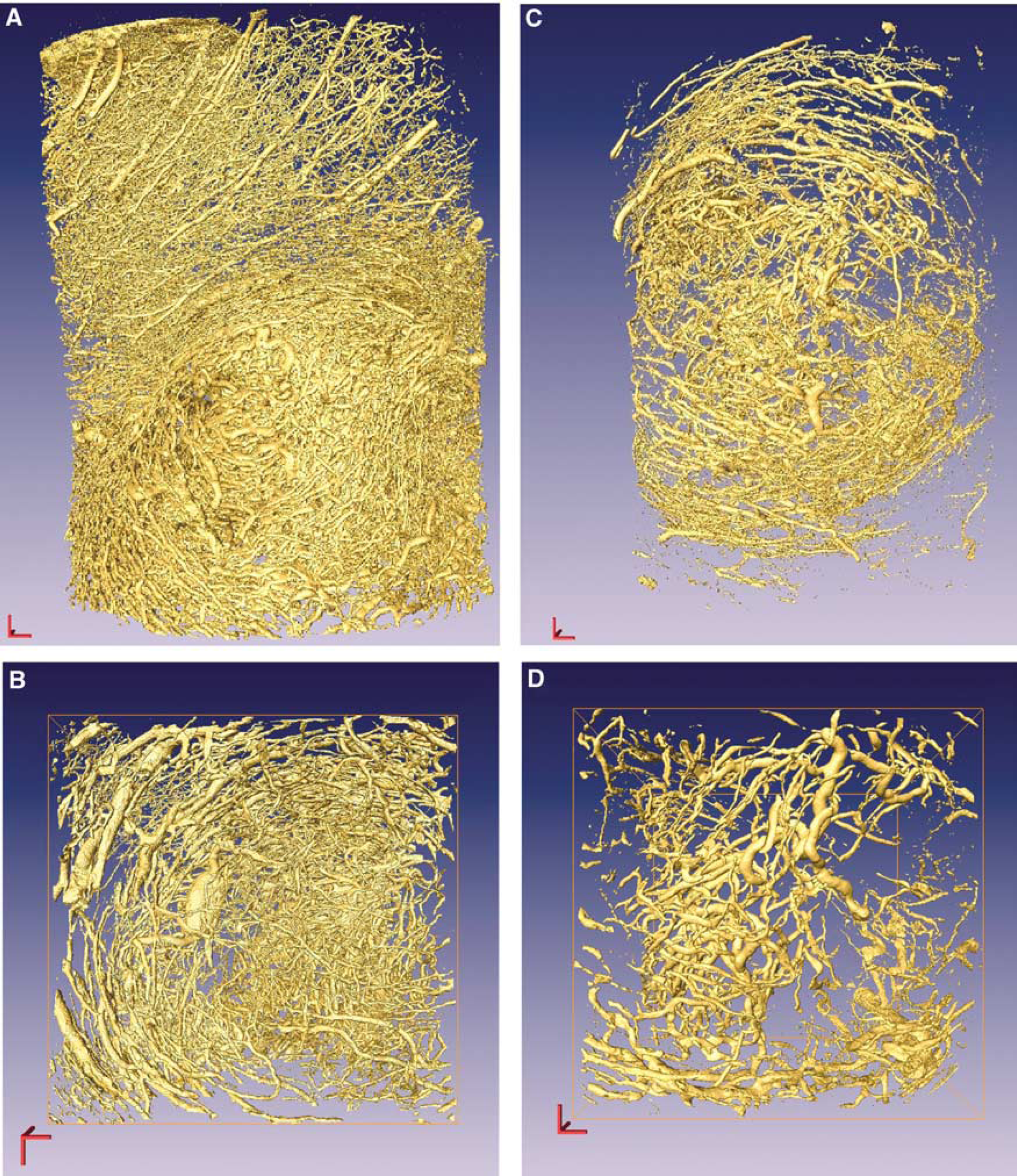
Volume rendering of an implanted tumor cortical vascular network in rat cortex for samples T₁ (A,B) and T₄ (C,D). Same conventions as in Figure 1.

Data Processing

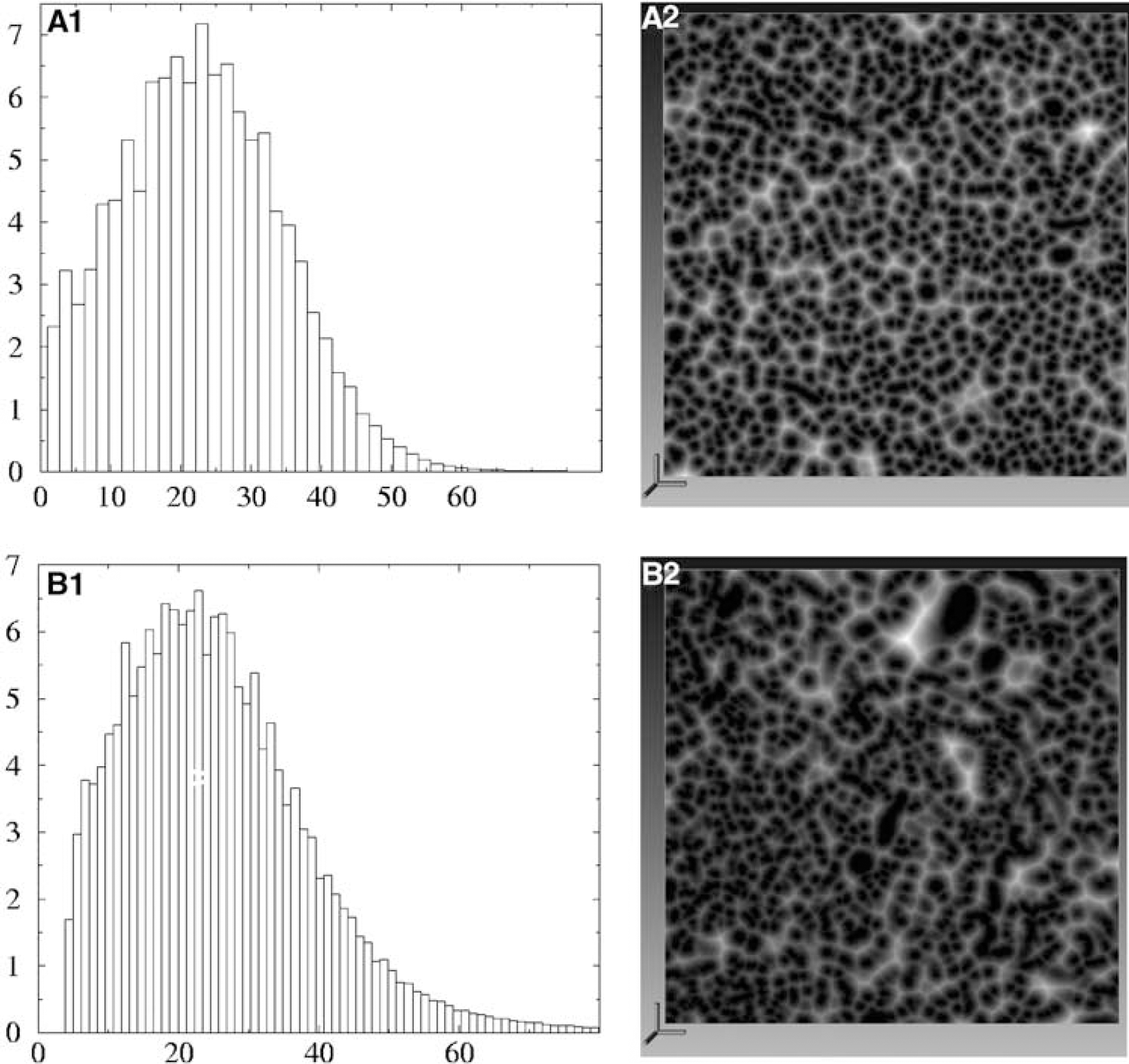
We applied different multiscale analyses to the binary images. Conventional box-counting and sand-box fractal analyses (Gazit et al, 1995; Feder, 1988) were used. We do not give details of these methods here as many textbooks and papers explain their principles and implementation (see, e.g., Feder, 1988). As a complement to these approaches, we also analyzed the distance map of the resulting network. The distance map represents the distance of any black voxel (tissue point) of the image from the nearest vessel, that is, the nearest white voxel, when considering binary images. Hence it quantifies the α-vascular space inside the cerebral tissue. Any white voxel has an associated distance equal to zero. The distance d(i,j,l) was computed in three dimensions along the discrete Cartesian coordinates based on the image voxels. This distance is interesting as it gives a quantitative measurement of the spatial distribution of the vascular network inside the cortical tissue. By computing how ‘far’ any point in the neural tissue is from the vascular network, one can obtain insights into the spatial distribution of oxygen by the vascular network and how the network drains metabolic products. It is interesting to note that this information cannot be retrieved from a simple cumulated histogram of the distance map, which only describes how variable the distance to any vessel is. The comparison between the distance maps of healthy (Figure 3A1) and tumorous tissue (Figure 3B1) shows that the typical vessel/tissue distances, associated with the histogram's mode, are very similar, about 22 μm. Nevertheless, the information contained in this histogram smears-out the existence of large or small, poorly or densely vascularized local regions. Figure 3A2 and 3B2 give two examples of two-dimensional sections through the 3D distance map. The comparison of the figures first shows that both vascular networks display a wide distribution of dense (black) or loose (white) local vascular density. This is the signature of some scale-invariance on the small scale.

Figure 3

(A1,B1) Normalized histograms of the 3D distance map d in micrometer computed for the monkey microvascular cortex shown on Figure 1 in (A1) and the implanted tumors in rat brain shown on Figure 2 in (B1). (A2,B2) Representation of the corresponding 3D distance map projected in a (x, z) plane, coded in gray scale between white for maximal distances to black for minimal distances equal to 0. Three dimensional scale-bar is 100 mm in each direction.

Nevertheless, tumor distance maps (Figure 3b2) look much more heterogeneous than normal ones (Figure 3b2). Hence, while the average vessel/tissue distance of tumorous and normal microvascular networks is quite similar, the local vessel density is significantly different. This property can be further quantified by computing the correlation function of the distance map d(i,j,l) also called covariance function in statistics. It gives a quantitative estimation of the correlation of the distance map at a given distance along the discrete grid directions x,y, or z. This correlation permits the quantification of the qualitative texturing of the distance map field observed on Figures 3a2 and 3b2. Moreover, the way this texturing varies in space is related to the variations of the correlation function with the distance, as precisely quantified by the covariance function. But the computation of this covariance function is difficult in three dimensions (it requires the evaluation of a convolution product in each dimension of space). It becomes almost impossible with a single computer when images as large as those obtained from our acquisition are involved (e.g, 1024 × 1024 × 1024 voxels). The conventional way around this technical difficulty is to consider the Fourier transform of the distance map, which we will note d͠(k_i, k_j, k_l) As a matter of fact, the modulus of the Fourier transform |;d͠(k_i, k_j, k_l)|; ² is closely related to the Fourier transform of the covariance of the distance map (according to Wiener–Kintchine theorem). Hence, computing the modulus of the Fourier transform, also called the power spectrum P(k_i, k_j, k_l) = |;d͠k_i, k_j, k_l |;² gives the same information about the spatial distribution of the correlation as computing the covariance. As the computational cost of 3D Fourier transformations is very reasonable when fast-Fourier transform methods are used, in the following we will consider the Fourier spectrum of the distance map. For that purpose the distance map d(i, j, l) is periodized in each direction of space so as to prevent aliasing artifacts. This method is widely used in many practical applications for the investigation of multiscaled properties of random signals (Feder, 1988; Plouraboué and Boehm, 1999). In three dimensions, it is a very powerful method as it permits the analysis of the possible anisotropy of the multiscaled properties, as opposed to the fractal box counting methods.

Results

Imaging

Healthy and tumorous vascular networks present distinct structural properties, whereas no significant differences could be observed between healthy marmoset monkey and rat tissue. The vessel density observed in Figures 1 and 2 illustrates the quality of the preparation. The apparent high density results from the projection over a thickness of 2.5 mm. The average vessel volume density is smaller for the normal monkey vascular network of Figure 1B (2%) than for the tumor of Figure 2B (5.7%). Moreover, the vessel diameter distributions are different: 80% of the normal cortical vascular network of Figure 1B has a diameter smaller than 10.4 mm whereas this value reaches 24.4 mm for the tumorous vessels of Figure 2B. The values are only illustrative, as the systematic comparison of such local parameters is not the purpose of our study. The vertical z-axis of the image is approximately perpendicular to the cortex surface so that the large vessels in the upper part are pie-merial. Normal vascular networks show conspicuous large arteriolar and venular columns whose orientation is approximately orthogonal to the cortex surface. This anisotropy of the normal vascular cortex in primate was generic for all the cortical regions investigated. Normal rat cortex has similar properties (see, for e.g., Plouraboué et al, 2004). However, implanted tumors present rather concentric vascular networks, as illustrated in Figure 2B. This is consistent with an expansion mode of implanted tumor, which develops from the central injection point. Moreover, it can be seen that the local vessel density at small scale varies more in Figure 2B than in Figure 1B. This qualitative observation will be further investigated quantitatively using fractal analysis and the distance map power spectrum.

Fractal Analysis

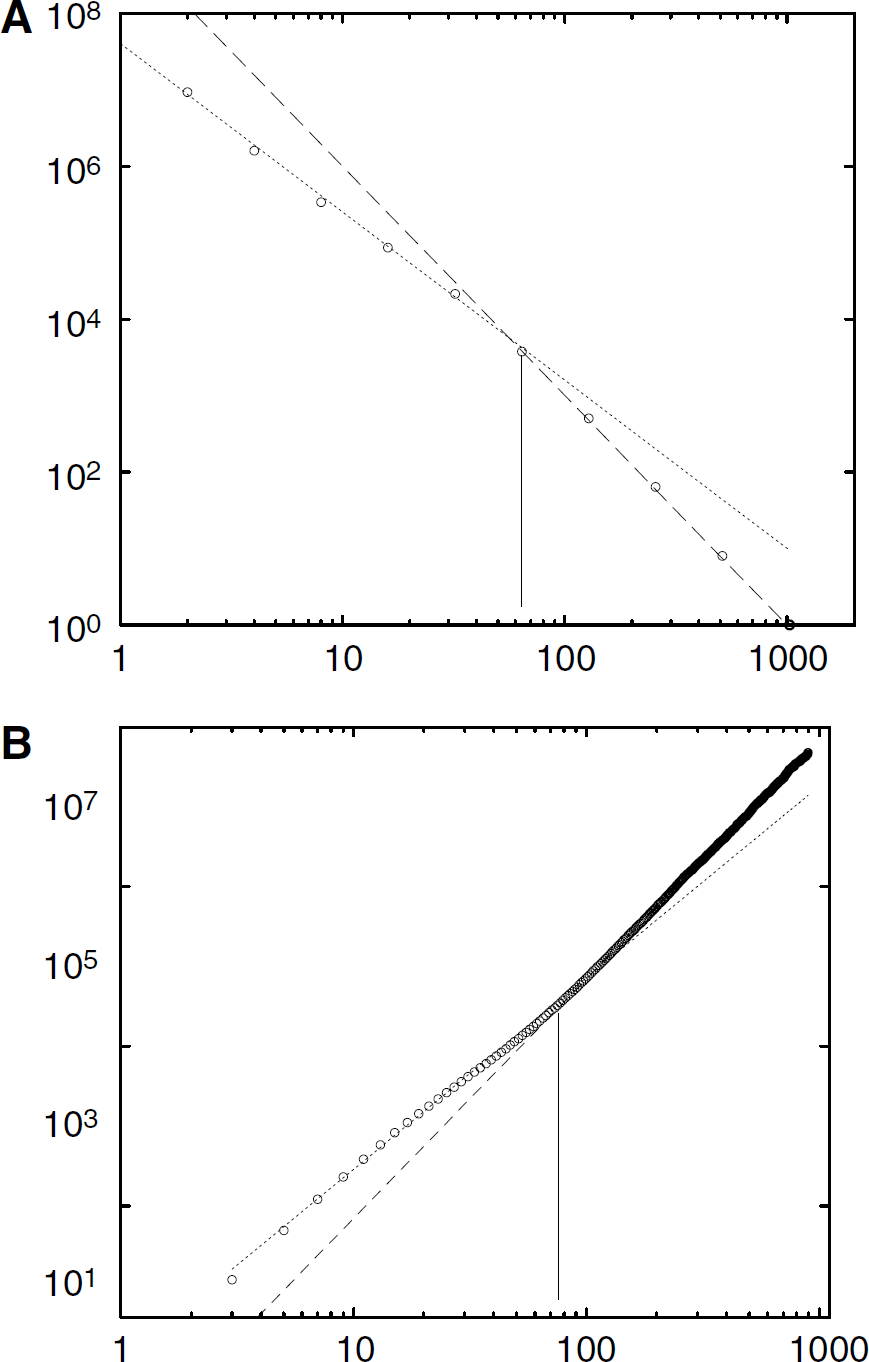
The box-counting and sandbox methods used in Figures 4 and 5 illustrate two generic properties. On the small scale, the microvascular network shows a multiscale fractal behavior between the voxel size (1.4 mm) to some upper cutoff cc. It can be observed that the use of very large data sets for the fractal analysis leads to clearcut linear trends with very small error bars in the estimated slopes. Above this lengthscale, the 3D vascular network appears as a homogeneous 3D object associated with the cubic behavior of both curves. Hence, cc gives the scale above which the vascular network can be considered as homogeneous and can no longer be considered as multiscaled. In the porous media literature, such a scale is called a REV lengthscale. This lengthscale is important as it could be considered as the one associated with some vascular modular spatial extension. In fact, this scale has been found to be larger in tumorous microvascular networks than in normal ones. For example cc is equal to 42 and 56 μm in Figures 4A and 4B and to 88 and 91 μm in Figure 5A and B, respectively. All the other results are presented in Table 1. These properties are self-consistent with the results obtained from the distance map analysis given below.

Figure 4

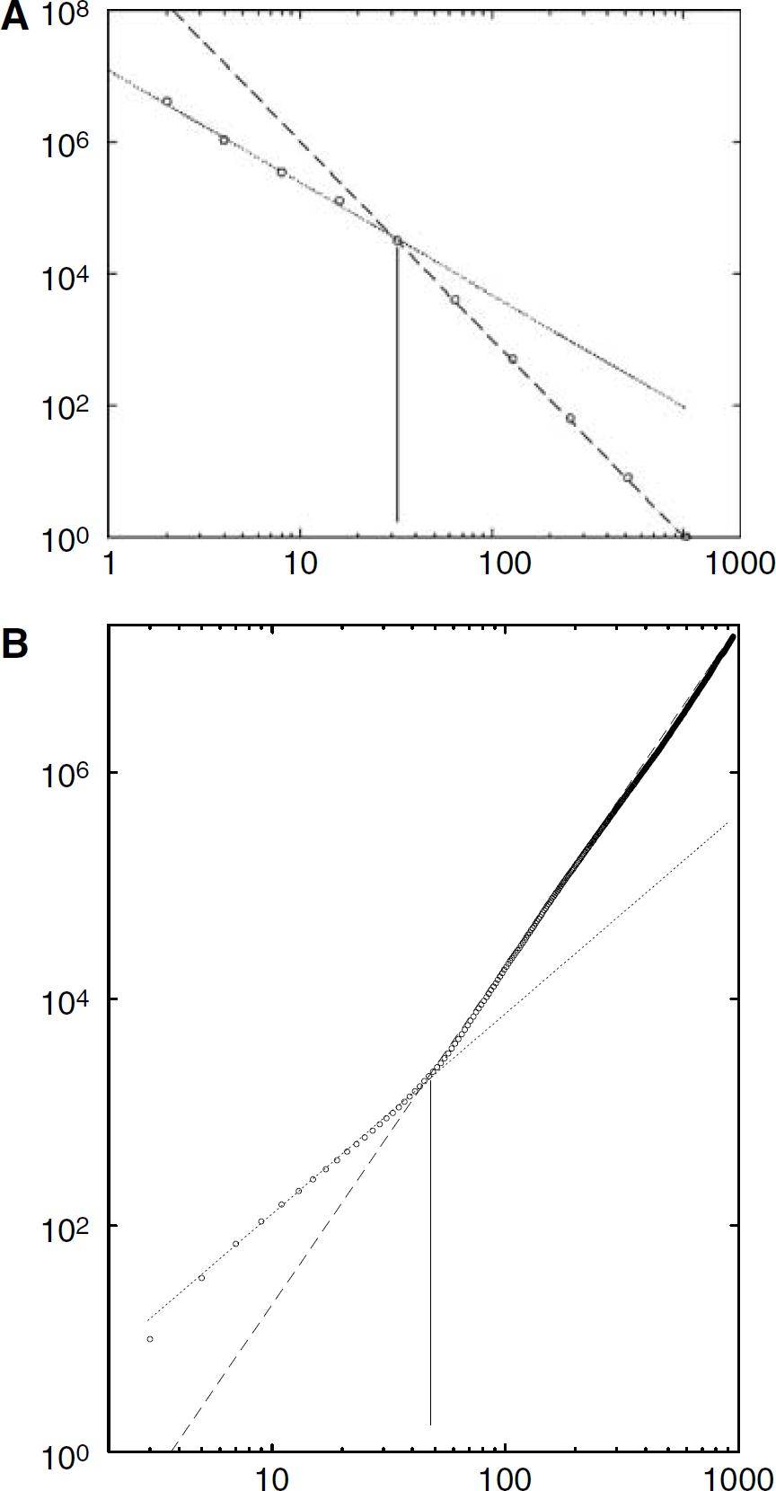
Fractal analysis on the vascular network of marmoset sample M₁ shown in Figure 1. The fractal regime is represented by a dotted line, while the homogeneous regime associated with a slope equal to 3 is plotted with long dashes. (A) Box-counting method in bi-logarithmic coordinates where the scale Δ is in voxel units. The slope of the dotted line leads to a fractal dimension equal to 1.7±0.1. (B) Sand-box counting method. The slope of the dotted line leadsto a fractal dimension equal to 1.8±0.1.

Figure 5

Same conventions as Figure 4 applied to the vascular network of tumorous rat sample T₁ shown in Figure 2. (A) The slope of the dotted line leads to a fractal dimension equal to 2 ± 0.1. (B) The slope of the dotted line leads to a fractal dimension equal to 2.2 ± 0.1.

A-Vascular Space Analysis

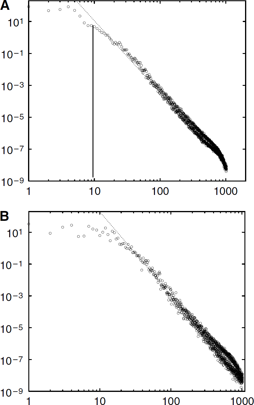
The power spectrum of the distance map was used to investigate the spatial distribution of the nonvascularized tissue. Both (x, y) and z directions were analyzed separately to look for any anisotropic properties of the vascular network. Figure 6 shows both types of spectra, which display the same generic properties. For large wavelengths, corresponding to small scales, the distance map has a power-law behavior |;d͠|;² ~ k^−v. The exponent v of this power law is different in the (x, y) and z directions. For example in the case of Figure 6 obtained on data of the sample shown in Figure 1 associated with marmoset normal vascular network, the power-laws are |;d͠|;² ~ k_XY^−4.9 and |;d͠|;² ~ k_Z^−5.3, respectively, in the (X, Y) and Z directions. This behavior is consistent with the observed anisotropy of normal cortical vascular networks shown in Figure 1, for which the Z direction perpendicular to the cortex surface displays highly correlated structures associated with vascular cortical columns. This anisotropy is still observed on tumorous vascular networks, for which the power-law observed in the (X, Y) and Z directions of Figures 7A and 7B are, respectively, |;d͠|;² ~ k_XY^−4.3 and |;d͠|;² ~ k_Z^−5.2. This property was confirmed on each tumorous sample that was analyzed in the same way, as described in Table 1. Furthermore, below some critical wavelength, the Fourier spectrum saturates. This saturation is associated with a lower cutoff of the Fourier spectrum, which is directly related with the correlation length ℓ, as indicated in Figures 6 and 7. Table 1 gives the comparison between this correlation length ℓ and the REV length-scale ℓ_c estimated from the Fractal analysis. ℓ and ℓ_c are complementary measurements of a similar network property, the scale above which either the vascular density or the vascular distance can be considered as homogeneous.

Figure 6

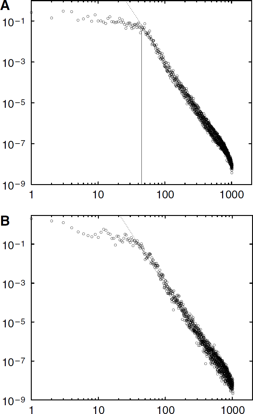
Averaged power spectra |;d͠|;²(k) of the distance map computed for the vascular network of Figure 1 in bi-logarithmic coordinates. The vertical line indicates the wavelength cutoff associated with the power law behavior (A) versus ( $k_{xy}=\sqrt{k_x^2+k_y^2}$ ) and (B) versus k_Z.

Figure 7

Same conventions as Figure 6 for the distance map of the tumorous vascular network of Figure 2.

Statistical Analysis

First, it can be qualitatively observed that both ℓ (obtained from the Fourier spectrum) and ℓ_c (obtained from the fractal box counting method) are positively correlated, the degree of correlation nevertheless depending on the fractal analysis method. A correlation coefficient r =0.9 was found between ℓ and ℓ_cBC and r = 0.66 for ℓ_cSB. In both cases, the correlation was found statistically significant at the 5% level. Moreover, comparing the measurements of ℓ and ℓ_c in Table 1 on normal tissues either in rat (R_i, i =1,2 samples) or in marmoset (M_i, i =1….5 samples) with measurements on implanted tumor networks (T_i, i =1…4 samples) seems to indicate that tumor vascular networks are fractal over much larger scales. We have then investigated the statistical relevance of this observation. Using a Wilcoxon rank test we first tested, for the three parameters ℓ, ℓ_cBC and ℓ_cSC the possible equality between R_i and M_i samples. None of the parameters was found to be significantly different at the 5% level. Using this first result, the data associated with R_i and M_i samples were combined, and their possible equality with tumor samples T_i tested. We found a highly significant difference for all three parameters ℓ, ℓ _cBC and ℓ _cSC with an associated probability of 0.3% much smaller than the 5% level.

Another interesting question about Table 1 is whether the observed fractal dimensions are different for healthy and tumorous vascular networks. A similar Wilcoxon rank test was applied to both BC and SB measurements. In the same way we first tested the equality of fractal dimensions measured for R_i and M_i samples. Neither D_BC nor D_SB were found to be significantly different with associated probability of 30% and 9% both larger than the 5% level. However, when the fractal dimensions obtained for R_i and M_i samples were combined and the equality with tumor samples T_i was tested, a very significant difference was found, associated with a probability 0.03% much smaller than the 5% level. From this, it can be concluded that the fractal dimension associated with tumorous vascular networks is significantly larger than those measured on healthy vascular networks.

Finally, we also analyzed the surface to volume ratio of the vascular network reported in the last column of Table 1. A statistical analysis of these data using a Mann–Whitney test shows that the Marmosets sample M_i, i = 1‥5 and the healthy rat R_j, j =1,2 cannot be considered as different with an associated probability P =0.12 larger than the 5% level. As previously we have then agregated the M and R groups and then tested their difference with sample T_i, i= 1‥4. We found a significant difference between both with an associated probability P= 0.038. We then conclude that the surface exchange of vessels in tumour is larger than in healthy tissues.

Discussion

From the results obtained, we can conclude that both tumorous and healthy brain vascular networks display a fractal organization on small scale. To our knowledge, this observation is new and results from the high quality of the 3D spatial resolution of the images obtained. Previous analysis (Gazit et al, 1995; Baish and Jain, 2000) performed using lessaccurate spatial resolution had concluded that a healthy cerebral vascular network did not present multiscale behavior. We indeed reached the same conclusion when considering lengthscale larger than 50 to 80 mm. This analysis gives an explanation for the apparent contradiction previously found in the literature concerning multiscale properties of healthy vascular networks. The point should nevertheless be raised that most of the measurements were carried out on biological tissue preparations whose properties could differ with those of in vivo tissues. In our experimental protocol, we found a 20% to 30% shrinkage of the tissue volume which might have affected some of the results presented. As the relative volume of the vascular network in the tissue is 2% to 3%, a shrinkage of the tissue volume of 20% to 30% would hardly change the vascular density by more than 0.7% in the worst case for which the vessels would not be affected by the volume shrinkage. Nevertheless, we expect that as the volume shrinkage is essentially associated with the removal of water from within tissue, the percentage of volume lost inside the vessel should be equivalent to that of the tissue. Thus, the shrinkage of the vessels should be equivalent to that observed in the tissue, and their relative density should not change. Moreover, even if the vessels were not affected by the volume shrinkage, so that their relative density is increased by 0.7% we would not expect changes in the multiscale properties that were investigated. This is because the fractal dimension associated with the vascular density does not depends on the intrinsic value of the density but rather on the scale-dependence of this quantity. As the volume shrinkage would affect each length-scale in a equivalent manner, it should not influence the multiscale distribution of the vascular density.

The lengthscale for which this transition between fractal to nonfractal occurs defines the REV of the vascular structure, which has been quantified for different cortical regions in the primate cortex. The evaluation of this REV lengthscale in normal cerebral tissue is an important parameter in many contexts. For example, one has to bear in mind that most cerebral imaging techniques such as magnetic resonance imaging or PET-scans have spatial resolution close to 1 mm³ (maybe one-half in the most favorable cases. Hence, the vascular structure contained in one voxel of these functional images corresponds to the highly complicated structure presented in Figures 1B or 1D. Our analysis indicates that this vascular network can be decomposed in decorrelated 50 to 80 mm cubic units of volume in normal tissues, which defines the scale for 3D vascular modules in primate cortical gray matter. It is interesting to note that the observed statistical variations of this parameter were not significantly different from those observed on rat normal cortex. This observation is important in the recent context of high-resolution imaging techniques for small animals, as well as for the extrapolation to humans of studies obtained from rat cortex. In contrast, we observed that the REV lengthscale was significantly smaller in healthy tissues than in tumorous ones. In the latter, the REV lengthscale parameter ℓ associated with the distance map homogeneity scale was as large as several hundreds of micrometers. We obviously think that this parameter depends on the tumor's development. It is therefore an interesting parameter for quantifying the ‘normalization’ of a tumor vascular network (Jain, 2005). Moreover, the fractal dimension observed in tumors was statistically larger than in healthy tissues. This characteristic might be related to the need for a larger nutrient supply to the more intense tumor metabolism. It is to be expected that the nutrient transfer from the vascular system to the tumorous tissue increases as the surface exchanges increase. At a given scale L smaller than the REV lengthscale ℓ, the surface exchange is precisely proportional to L^D−1, where D is the fractal dimension associated with the vascular network. One should nevertheless argue that this scaling relation does not necessarily mean that the surface exchange of the vessels is larger in tumour because it does not take into account the coefficient of proportionality. To address this issue, we have then checked directly from our images the surface exchange of the vessels. The statistical analysis of the values reported in the last column of Table 1 has shown that the surface exchange of vessels in tumor is larger than that in healthy tissues. This confirms the idea that a larger fractal dimension is associated with a larger surface exchange in the vascular networks that have been analyzed, and so possibly a larger metabolic supply. This is obviously only one element among others which characterizes the transfer from blood to the brain tissue. Even if the transfer of gas molecules such as oxygen or carbon dioxide is passive some nutrient fluxes are often limited spatially and temporally by protein transporters on the vasculature. Hence the relevance of surface exchange for the quantification of nutrient fluxes has to be regarded with some care. The results obtained could also give new insights to improve previous models proposed to relate vascular architecture and nutrient delivery in tumors (Baish et al, 1996).

Finally, we would like to point out that the 3D images obtained in this work could be useful for investigating the underlying cortical hemodynamics. One interesting study would be to investigate how multiscaled spatial properties of CBF might lead to some temporal fluctuations of the CBF, the Fourier spectrum of which could be compared to experimental measurements (Eke et al, 2005). Conversely, the question of how and when CBF changes could affect the fractal properties of cortical vasculature would also be interesting.