Sage Journals: Discover world-class research

Abstract

Dynamic positron emission tomography (PET) data are usually quantified using compartment models (CMs) or derived graphical approaches. Often, however, CMs either do not properly describe the tracer kinetics, or are not identifiable, leading to nonphysiologic estimates of the tracer binding. The PET data are modeled as the convolution of the metabolite-corrected input function and the tracer impulse response function (IRF) in the tissue. Using nonparametric deconvolution methods, it is possible to obtain model-free estimates of the IRF, from which functionals related to tracer volume of distribution and binding may be computed, but this approach has rarely been applied in PET. Here, we apply nonparametric deconvolution using singular value decomposition to simulated and test–retest clinical PET data with four reversible tracers well characterized by CMs ([¹¹C]CUMI-101, [¹¹C]DASB, [¹¹C]PE2I, and [¹¹C]WAY-100635), and systematically compare reproducibility, reliability, and identifiability of various IRF-derived functionals with that of traditional CMs outcomes. Results show that nonparametric deconvolution, completely free of any model assumptions, allows for estimates of tracer volume of distribution and binding that are very close to the estimates obtained with CMs and, in some cases, show better test–retest performance than CMs outcomes.

Keywords

binding full quantification model-free PET singular value decomposition

INTRODUCTION

Positron emission tomography (PET) is a nuclear imaging technology that uses radioactively labeled molecules (tracers) that are injected into the body and bind, although not exclusively, to a specific target to quantify in vivo biological processes, such as blood flow, metabolism, and the distribution of proteins in the brain and the body. PET is an invaluable tool to establish the genetic and cellular basis of diseases.

Fully quantitative PET allows estimation of outcome measures such as, in the case of a reversible tracer, the total volume of distribution (V_T) of the injected tracer and a series of binding potentials (BPs) between tracer and target, to indirectly determine the available amount of the target.¹ These BPs are in various ways related to the density of available target (B_max) through the affinity of the tracer for the available binding sites (1/K_D).¹

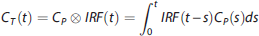
Quantification of these outcome measures relies on describing the PET signal associated with the tracer in the tissue (i.e., the time activity curve, TAC) as the convolution between the concentration of free (not protein bound) unmetabolized tracer in the arterial plasma (i.e., the metabolite-corrected input function) and a function specific to the tissue, the impulse response function (IRF).² The metabolite-corrected input function represents how much of the injected tracer is actually available to bind with the target. IRF is estimated from measures of the input and the tissue PET signal, and would not otherwise be known.

Traditionally, PET quantification methods have used parametric approaches, which require specifying a certain parametric form for the IRF (e.g., a mathematical function derived from a physiologic model of the system, or that approximates the system behavior). This approach therefore relies on fairly strong assumptions, which are not always substantiated in reality, and a priori knowledge of the system under investigation. Traditional PET parametric analysis quantifies these outcome measures by interpreting the PET signal in the brain tissue using compartment models (CMs) to describe the system IRF (the kinetics) of the tracer, in particular a reversible or irreversible two-tissue compartment model (2TCM).¹ The tracer signal in the brain tissue is modeled as the sum of two components: part of the tracer is specifically bound to the target of interest (specific binding); part is nonspecifically bound to macromolecules other than the target, or free in the tissue water (nonspecific binding).^1,2 Identification of this model involves estimating four rate constants (K₁, k₂, k₃, k₄), which describe how quickly the tracer transits from ‘being in the plasma’, to ‘being free to bind in the tissue’, to ‘being specifically bound to the target’.^1,2 However, these constants are not always all identifiable, and as a result directly estimating the specific binding component in the model can often be unstable. Therefore, full quantification of this model also requires identifying a reference region (RR) in the brain that is completely devoid of the target.^1,2 In a proper (i.e., measurable, valid, reliable, independent of treatment effects and groups) RR devoid of the target of interest, the tracer can only be nonspecifically bound to macromolecules other than the target,^1,2 and its kinetics can be described with a one-tissue compartment model¹ (1TCM) regulated by only two rate constants (K₁′ and k₂′). The tracer volume of distribution in such a region is assumed to represent (and used to estimate) a common nonspecific binding across the brain, and helps isolate the component that is only specifically bound to the target. Often, however, CMs or graphical approaches derived from CMs² either do not properly describe the tracer kinetics, or are not identifiable, leading to nonphysiologic estimates of the V_T and of the binding to the target.

On the other hand, nonparametric deconvolution approaches do not impose any specific formulation or model for the IRF, and only rely on very loose requirements, often matched in the case of physiologic systems, for the IRF (e.g., degree of smoothness; monotonicity). Nonparametric deconvolution approaches, therefore, allow obtaining model-free estimates of the IRF, from which functionals related to tracer V_T and BPs can be computed. Nevertheless, they have been rarely adopted in PET. O'Sullivan et al³ proposed the use of nonparametric residue analysis and demonstrated it with simulations and data using the irreversible tracer [¹⁸F]FDG. Only recently, Jiang et al⁴ proposed a nonparametric approach based on functional principal component analysis and demonstrate it with simulations and data with the tracer [¹¹C]-diprenorphine.

Several approaches have been developed that fall between these two extremes.^5–7 Generally, these involve expressing the IRF in terms of basis functions that, although derived from the principles of linear time-invariant systems and based on CMs,⁸ do not impose any predefined compartmental structure. Similar to what we propose using nonparametric deconvolution approaches, these basis function approaches allow for calculation of functionals that can be computed from the IRF as PET outcome measures.

Here, we propose the use of nonparametric deconvolution via singular value decomposition (SVD)^9,10 to compute functionals of the IRF of PET reversible tracers that are associated with tracer V_T and BPs, and extensively compare accuracy, reproducibility, reliability, and identifiability of these different functionals with traditional outcome measures derived using CMs. SVD is an easy-to-implement nonparametric deconvolution approach that is widely used, for example, in the quantification of Dynamic Susceptibility Contrast-Magnetic Resonance Imaging data^9,10 and has been used before to obtain regularized least-square solutions.^7,11–13 We show relative advantages and disadvantages of using outcome measures derived from either nonparametric deconvolution or traditional parametric approaches, using simulated data and four test–retest clinical datasets with the tracers [¹¹C]CUMI-101 (CUMI), [¹¹C]DASB (DASB), [¹¹C]PE2I (PE2I), and [¹¹C]WAY-100635 (WAY).

MATERIALS AND METHODS

SUBJECTS

Four previously acquired test–retest datasets were considered: 12 scans with CUMI,¹⁴ 20 with DASB,¹⁵ 14 with PE2I,¹⁶ and 10 with WAY.¹⁷ The studies were performed in accordance with the Declaration of Helsinki and The Institutional Review Boards of Columbia University Medical Center and New York State Psychiatric Institute approved the protocol. Subjects gave written informed consent after receiving an explanation of the study.

Positron Emission Tomography Protocol

Tracers preparation, emission data acquisition and reconstruction, and determination and fit of the metabolite-corrected input function were obtained as previously described.^14–17

Image Analysis

Images were analyzed using Matlab Release 2013b (The Mathworks, MA, USA) with extensions to FLIRT version 5.2 (ref. 18) and BET version 1.2 (ref. 19). Motion correction was applied. An RR and several anatomic target regions of interest (ROIs) were traced based on brain atlases and published reports:^20,21 13 ROIs for CUMI (hippocampus, entorhinal cortex, insula, posterior parahippocampal gyrus, temporal lobe, amygdala, medial prefrontal cortex, cingulate, orbital, dorsolateral prefrontal cortex, parietal, raphe, occipital lobe; RR: cerebellar gray matter); 6 ROIs for DASB (midbrain, anterior cingulate, amygdala, dorsal putamen, hippocampus, thalamus; RR: cerebellar gray matter); 4 ROIs for PE2I (dorsal caudate, dorsal putamen, ventral striatum; RR: cerebellum); and 13 ROIs for WAY (raphe; anterior cingulate; amygdala; cingulate, dorsolateral prefrontal cortex, hippocampus, insula, medial prefrontal cortex, occipital lobe, orbital, parietal, posterior parahippocampal gyrus, temporal lobe; RR: cerebellar white matter). Selecting these ROIs restricted the analysis to regions for which the binding is expected to be relatively high (with the exception of the RR).

Simulated Data

In addition to the clinical test–retest data sets, we considered simulations designed to generate data that imitate characteristics of real data in the case of 1TCM and 2TCM, respectively.

For the 1TCM, we used the metabolite-corrected input function measured in one of the considered DASB scans, a tracer whose kinetics is well described by a 1TCM,¹⁵ and set the K₁ and k₂ values in six selected regions (cerebellar gray matter, temporal lobe, hippocampus, dorsal caudate, amygdala, and ventral striatum) based on existing data on DASB healthy control subjects.¹⁵ For the 2TCM, we used the metabolite-corrected input function measured in one of the considered CUMI scans, a tracer whose kinetics is well described by a 2TCM,¹⁴ and set the K₁ to k₄ values in five selected regions (cerebellar gray matter, hippocampus, temporal lobe, occipital lobe, and cingulate) based on existing data on CUMI healthy control subjects.¹⁴

In both cases, we simulated Gaussian noise with zero mean and standard deviation (SD) calculated as SD(t_i) = α. σ/w(t_i), where w(t_i) is the root square of the duration of the time frame during which the PET data corresponding to time t_i has been acquired, and σ indicates the level of noise that we derived from the weighted residual sum of square values obtained by fitting DASB and CUMI scans, respectively, with CMs. Increasing α allows us to study the various estimation techniques in situations with proportionately more noise than what we encounter in our real-data situations. We simulated five noise conditions setting α equal to 1, 2.5, 5, 7.5, and 10, respectively. In all cases and noise conditions, we simulated 1,000 TACs for each of the selected regions.

The complete list of simulated parameter values and noise levels is reported in the Supplementary Material.

Interpretation of Positron Emission Tomography Data

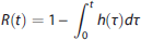
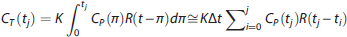
The PET data are commonly modeled as a convolution of the metabolite-corrected input function and the tracer IRF in the tissue:²

C_{T} (t) = C_{P} \otimes I R F (t) = \int_{0}^{t} I R F (t - s) C_{P} (s) d s

(1)

where C_T(t) is the PET tracer TAC in an ROI or voxel and C_P(t) is the metabolite-corrected input function. In the case of 2TCM, IRF is a function of the K₁ to k₄ values of the corresponding CM, and is indicated here as IRF_CM:

I R F_{C M} (t) = K_{1} \cdot f (t; k_{2}, k_{3}, k_{4}) = K_{1} [π e^{- t a_{1}} + (1 - π) e^{- t a_{2}}]

(2)

where

a_{1 (2)} = \frac{1}{2} [k_{2} + k_{3} \pm k_{4} \pm \sqrt{{(k_{2} + k_{3} + k_{4})}^{2} - 4 k_{2} k_{4}}]

(3)

and

π = \frac{k_{3} + k_{4} - a_{2}}{a_{1} - a_{2}}

(4)

However, according to the theory of intravascular indicator dilutions, which was developed in the seminal work of Meier and Zierler²² and then extended to the general case of extravascular tracers (as in the case of PET) by O'Sullivan et al,³ an equation analog to (1) can be written:

C_{T} (t) = C_{P} \otimes I R F (t) = K \int_{0}^{t} R (t - s) C_{P} (s) d s

(5)

Equation (5) provides a probabilistic framework for representation of PET tracer data in terms of a convolution between the metabolite-corrected input function and a tissue residue function R(t). K is a proportionality constant, interpretable as an overall flow. The residue is a scaled survival function associated with tracer residence in the tissue. Physically, the residue function describes the fraction of indicator that remains in the tissue in response to an idealized bolus (Dirac delta function) input concentration at time t = 0. Initially, the residue must be unity (R(0) = 1) and from there it decreases (at least does not increase) as t increases. Assuming the residue is differentiable, it can be represented in the form:

R (t) = 1 - \int_{0}^{t} h (τ) d τ

(6)

where h(t) is a probability density function. Meier and Zierler²² developed an interpretation of h(t) in terms of the residence time distribution associated with an ensemble of capillary transport paths within the region. Indicator molecules are assumed to randomly sample such paths. Once a path is selected, the travel time of the molecule in the tissue is determined. Either due to flow, volume variations or binding, the transit time of the indicator in each transport path is considered to be distinct. From the distribution of transport paths there arises a distribution of transit times that would be experienced by a randomly chosen indicator molecule. The probability that an indicator molecule ends up on a path with transit time between t and t+Δt is proportional to h(t)Δt as Δt gets small. Hence if a collection of indicator molecules is introduced in trace amounts, so they do not interact, (6) gives the fraction of molecules that experiences transit times greater than t.

Outcome Measures

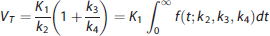
Expressing (1) as in (5), and considering nonparametric inference for the residue, gives rise to a deconvolution problem, providing a novel approach to the analysis of dynamic PET data that is not reliant on specific compartmental modeling assumptions.³ However, once the IRF has been nonparametrically estimated via deconvolution, it remains to establish which are the outcomes that can be actually computed from the IRF, and how they compare with respect to traditional outcomes used in PET. The first outcome measure usually computed in PET for a reversible tracer is V_T, whose formulation in terms of the 2TCM K₁ to k₄ values is:²

V_{T} = \frac{K_{1}}{K_{2}} (1 + \frac{k_{3}}{k_{4}}) = K_{1} \int_{0}^{\infty} f (t; k_{2}, k_{3}, k_{4}) d t

(7)

V_T equals the integral up to infinity of the corresponding IRF, which is only made possible by the parametric formulation of the IRF. When the IRF is computed nonparametrically, however, the IRF is estimated only up to the end time of the PET scan. A different definition is therefore necessary, as proposed by Jiang et al,⁴ in which a surrogate ‘volume of distribution’ for the tracer is calculated by integrating the IRF only up to the end time T_end of the scan:

V_{T - e n d} = K \int_{0}^{T_{e n d}} R (π) d π \neq V_{T}

(8)

To obtain a volume that is comparable to the approach used with CMs, O'Sullivan et al³ proposed an alternative formulation for V_T based on the idea that, if the residence density is partitioned into quantiles, the volumes occupied by fast, intermediate, and slow moving tracer label can be separately assessed.³ Their formulation uses the scaled first quantile of the residence density:

V_{T - N P 1} = \frac{K R^{- 1} (1 / 4)}{log (4)}

(9)

where R⁻¹(1/4) indicates the first quantile of the residence, which is the time at which the IRF reaches a fourth of its initial value, and the scaling log(4) ensures that if the residence density is exponential (i.e., as in the 1TCM case), then R⁻¹(1/4)/log(4) is equal to the mean of the residence distribution. The scaling factor in Equation (9) differs from the one reported in the paper by O'Sullivan et al.³ We closely checked our derivation of the scaling factor under the assumption that the residence density is exponential (h(t) = α × exp(– αt)). We confirmed our derivation using the reported clinical and simulated data. A closed-form expression for the scaling factor when the residence density is biexponential or more cannot be derived.

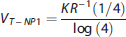
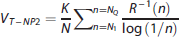
While the use of the first quantile of the residence was suggested for the irreversible tracer [¹⁸F]FDG,³ we propose here to further generalize and optimize this nonparametric formulation of V_T for reversible tracers, by considering not only the first quantile of the residence density (i.e., R⁻¹(1/4)), but also a large number of quantiles (i.e., R⁻¹(n), for n = N₁, ⃛, N_Q), and then averaging over all of them:

V_{T - N P 2} = \frac{K}{N} \sum_{n = N_{1}}^{n = N_{Q}} \frac{R^{- 1} (n)}{log (1 / n)}

(10)

This is a natural extension of the idea of tying the nonparametric estimate of the IRF with a particular counterpart; rather than relying only on a single estimated quantile with its inherent uncertainty, this approach will tend to ‘sharpen’ the estimator by considering many estimated quantiles with the expectation that the uncertainties will cancel each other out to some extent. Usually with CMs, once V_T is computed according to (7), the binding potential BP_P in any ROI/voxel can be indirectly estimated as BP_P = VT – V_Tref, where V_Tref is the tracer V_T in an RR devoid of the target of interest.¹ The same formulation of BP_P can be adopted for the V_T calculated according to Equations (8, 9, and 10), to obtain BP_P-end, BP_P-NP1, and BP_P-NP2, respectively.

Singular Value Decomposition

Potentially, any of many nonparametric deconvolution approaches can be used to estimate the IRF starting from known metabolite-corrected input function and tracer TACs in the brain tissue. O'Sullivan et al³ propose a technique based on regularized cubic B-spline approximation of the residence time distribution, but do not claim any optimality of the B-spline estimators. Jiang et al⁴ use functional principal component analysis. Here, we propose the use of SVD. Specifically, if the tissue concentration C_T(t) of the tracer in response to a metabolite-corrected input function C_P(t) is given by Equation (5), then assuming that the metabolite-corrected input function and the tracer TACs in the brain tissue are measured at equally spaced time points t₁, t₂, ⃛, t_N, with Δt as the space between time points of measurement, Equation (5) can be discretized, assuming that over short time intervals Δt, the residue function and metabolite-corrected input function are constant in time:

C_{T} (t_{j}) = K \int_{0}^{t_{j}} C_{P} (π) R (t - π) d π ≅ K Δ t \sum_{i = 0}^{j} C_{P} (t_{j}) R (t_{j} - t_{i})

(11)

K Δ t (\begin{array}{l} C_{P} (t_{1}) & 0 & \cdot \cdot \cdot & 0 \\ C_{P} (t_{2}) & C_{P} (t_{1}) & \cdot \cdot \cdot & 0 \\ \cdot \cdot \cdot & \cdot \cdot \cdot & \cdot \cdot \cdot & \cdot \cdot \cdot \\ C_{P} (t_{N}) & C_{P} (t_{N - 1}) & \cdot \cdot \cdot & C_{P} (t_{1}) \end{array}) (\begin{array}{l} R (t_{1}) \\ R (t_{2}) \\ \cdot \cdot \cdot \\ R (t_{N}) \end{array}) = (\begin{array}{l} C_{T} (t_{1}) \\ C_{T} (t_{2}) \\ \cdot \cdot \cdot \\ C_{T} (t_{N}) \end{array})

(12)

The requirement for equidistantly sampled data derives from the Shannon's sampling theorem,²³ which implies that any band-limited signal can be numerically reconstructed from its regularly spaced samples. The solution of the nonuniform sampling problem involves much more complex theoretical and computational issues (see Discussion).²⁴

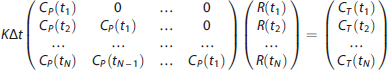
In matrix form, (12) is expressed as:

A b = c

(13)

where b contains the elements of R(t_i), i = 1, 2, ⃛, N, and c are the measured tracer TACs in the brain tissue C_T(t_i), i = 1, 2, ⃛, N.

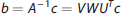
Equation (13) can be solved iteratively for the elements of b. This approach is, however, extremely sensitive to noise, potentially causing the estimated R(t) to oscillate. A technique to solve (13) is SVD, which constructs matrices V, W, and U^T, so that the inverse of A in (13) can be written:

b = A^{- 1} c = V W U^{T} c

(14)

where W is a diagonal matrix and V and U^T are orthogonal matrices. Given this inverse matrix, b, and consequently R(t), is calculated as

b = A^{- 1} c = V W U^{T} c

(15)

The main force of the SVD is that the diagonal elements in W are zero or close to zero corresponding to linear equations in (12) that are close to being linear combinations of each other. This fact thus allows one to identify elements in the matrix A that causes the solution b to oscillate or otherwise be meaningless in a biomedical modeling context. By eliminating (setting equal to zero) diagonal elements below a certain threshold in W, one can consequently minimize these effects before calculating b.²⁵

Here, we propose an automatic data-driven algorithm for selecting the threshold for SVD for each ROI that is based on cross-validation. Specifically, for each TAC in each considered ROI, the threshold is automatically selected by:

For i = 1 to i = N (with N the total number of original sampling time points)

Removing the TAC point corresponding to the sampling time point t_i;

For threshold T = 2% to T = 40% (with step = 1%), applying SVD with threshold value T to the TAC containing the remaining N – 1 data points;

Storing the threshold T that gives the best prediction of the TAC data at the time point t_i that was left out (i.e., calculated as the minimum of the square difference between original TAC value at the excluded time point t_i and the reconvolved TAC obtained with SVD at the same t_i);

Selecting the average value (across excluded time points t_i) of the stored thresholds.

The suggested threshold range is a generous range that has proven optimal before for physiologic signals.^9,10

Metrics of Comparison for Simulated Data

For all simulated cases and noise conditions, we ran SVD with the automatic threshold selection, and calculated V_T-NP1, V_T-NP2, and V_T-end from the deconvolved IRF estimates. BP_P-NP1, BP_P-NP2, and BP_P-end were derived by subtracting V_T-NP1, V_T-NP2, and V_T-end of the RR. We compared the distribution of outcome measures estimates obtained with the true simulated values, and calculated variance (across the 1,000 estimates of the outcome measure in each ROI, the median variance across ROIs is reported) and bias (as distance between median of the 1,000 estimates of the outcome measure in each ROI and the corresponding true value, the median bias across ROIs is then considered) of such outcome measures.

Application to Test–Retest Data

For all tracers, subjects, and ROIs, we calculated V_T and BP_P = V_T – V_Tref using CMs (2TCM for CUMI,¹⁴ PE2I,¹⁶ and WAY;¹⁷ 1TCM for DASB¹⁵); the RR was the gray matter (for CUMI¹⁴ and DASB¹⁵), the white matter (for WAY¹⁷), or the totality (for PE2I¹⁶) of the cerebellum. We also ran SVD with the automatic threshold selection, and calculated V_T-NP1, V_T-NP2, and V_T-end from the deconvolved IRF. BP_P-NP1, BP_P-NP2, and BP_P-end were derived by subtracting V_T-NP1, V_T-NP2, and V_T-end, respectively, of the RR.

We first compared V_T-NP1, V_T-NP2, and V_T-end versus V_T values using correlation (r), slope and intercept of the regression line, with V_T values being the independent variables. BP_P-NP1, BP_P-NP2, and BP_P-end were similarly compared with BP_P values.

We then compared the test–retest performance of V_T, V_T-NP1, V_T-NP2, V_T-end, and BP_P, BP_P-NP1, BP_P-NP2, BP_P-end, and using five metrics:¹⁵

Percent difference (PD), calculated as the absolute difference between the test and retest values divided by their average (the lowest the PD, the highest the reproducibility);

Within-subject mean sum of squares (WSMSS): WSMSS = $\frac{1}{n} \sum_{i = 1}^{n} \sum_{j = 1}^{2} [X_{i j} - {\overset{ˉ}{X}}_{i}],$ where X_i1 represents the ‘test’ value of an outcome measure for subject i, X_i2 the ‘retest’ value for the same subject, n is the number of pairs of subjects, and X_i = (X_i1 + X_i2)/2. This represents the variance in the estimation of a subject-specific outcome measure (the lowest the WSMSS, the highest the reproducibility);

Interclass correlation coefficient (ICC): ICC = $I C C = \frac{B S M S S - W S M S S}{B S M S S + (k - 1) W S M S S'}$ where BSMSS is the between-subject mean sum of squares ( $(B S S S = \frac{1}{n} \sum_{i = 1}^{2 n} \frac{1}{k} \sum_{j = 1}^{k} (X_{i j} - {\overset{ˉ}{X}}_{i}))$ ) and k is the number of repeated observations (k = 2 in this study; – 1 corresponds to no reliability, 1 to maximum reliability);

Variance of an outcome measure across subjects (sample variance, across subjects, of all observations for each ROI); and

Identifiability based on bootstrap resampling of residuals; we computed 100 bootstrap samples²⁶ of the TAC data for each subject's ROI, estimated the outcome measures for each of these samples, and measured the variability of these estimates using the robust median absolute deviation criterion: median [|Z_j – median(Z₁, Z₂, ⃛, Z₁₀₀)|, j = 1, 2, ⃛, 100].

RESULTS

Test–Retest Data

Comparison with CMs estimates. Figures 1 and 2 show for all tracers, subjects, and ROIs, the scatter plots of V_T-NP1, V_T-NP2, and V_T-end, and BP_P-NP1, BP_P-NP2, and BP_P-end, respectively, obtained using SVD versus the V_T and BP_P values obtained using CMs. The identity and regression lines, and the numerical results of the regression analysis, are reported in each plot. Correlation is high (> 0.90) in all cases, with exception of BP_P-NP1 for PE2I (r = 0.740) and BP_P-end for CUMI (r = 0.875).

Figure 1.

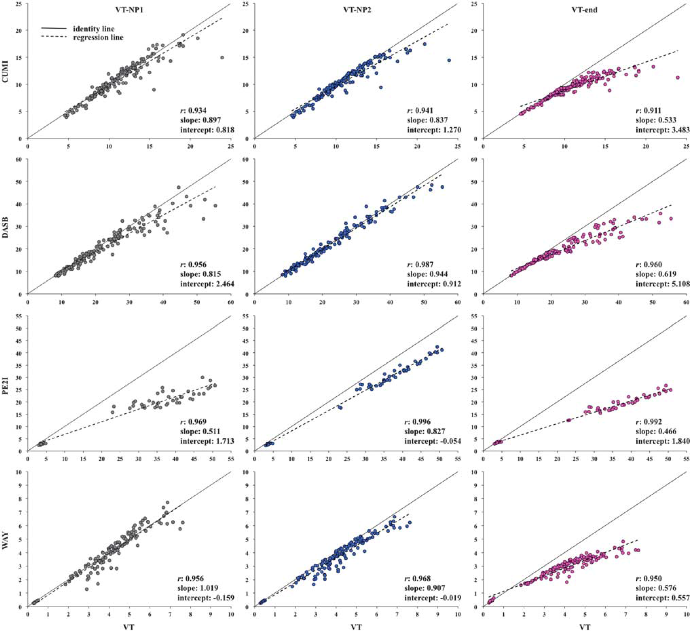
Scatter plots of V_T-NP1, V_T-NP2, and V_T-end obtained by singular value decomposition (SVD) versus the V_T values obtained using compartment models (CMs) for all considered tracers, subjects, and regions of interest (ROIs). The identity (solid) and regression (dotted) lines are reported in each plot, together with the numerical results of the regression analysis. V_T, total volume of distribution.

Figure 2.

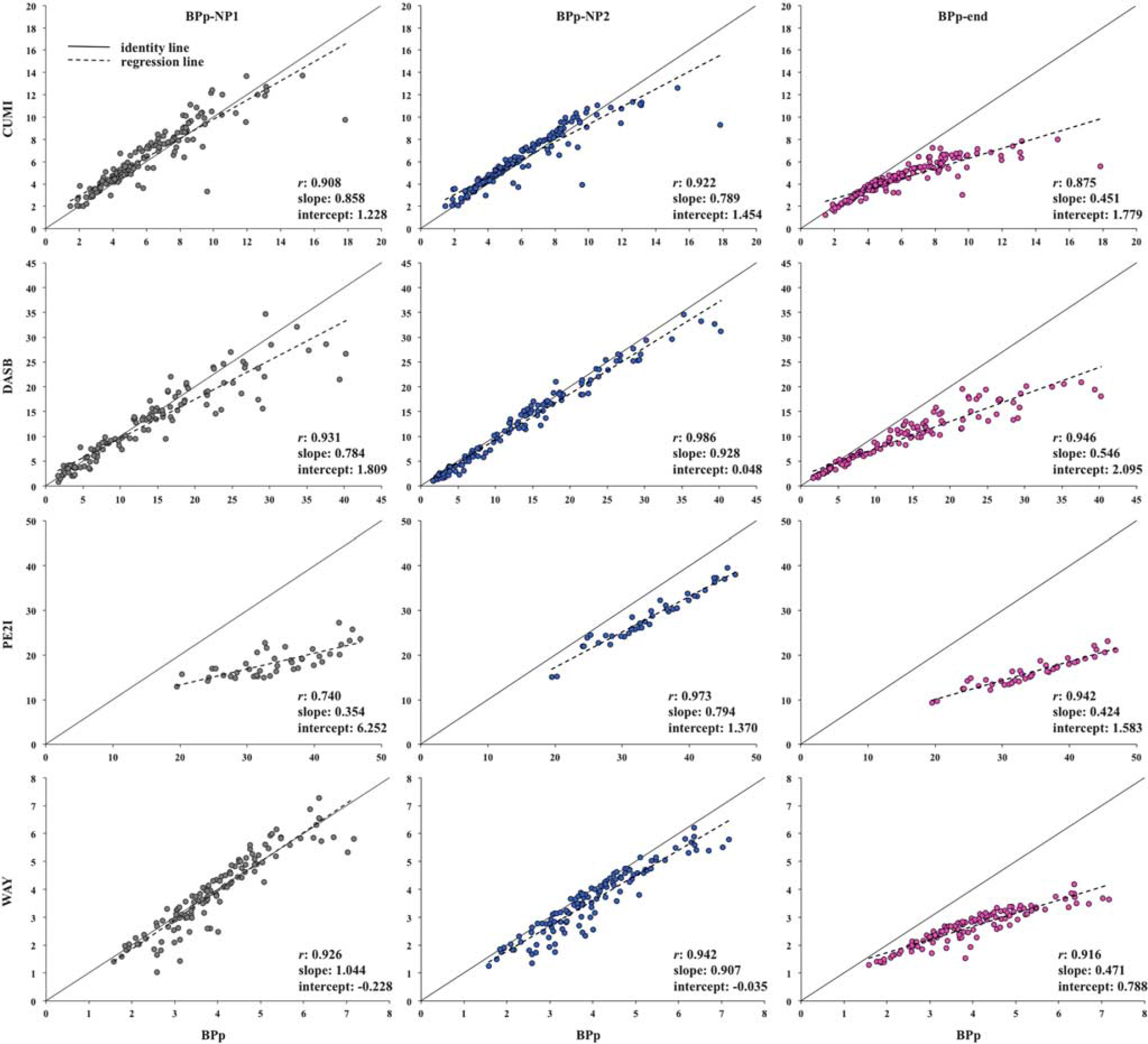
Scatter plots of BP_P-NP1, BP_P-NP2, and BP_P-end obtained by singular value decomposition (SVD) versus the BP_P values obtained using compartment models (CMs) for all considered tracers, subjects, and regions of interest (ROIs). The identity (solid) and regression (dotted) lines are reported in each plot, together with the numerical results of the regression analysis. BP_p, binding potential.

However, the slope values differ across outcome measures and tracers. As expected from its formulation in comparison with V_T, V_T-end underestimation increases as the value of the estimated outcome increases. V_T-end shows the lowest slope values across the different outcomes for all tracers: the minimum value is 0.466 (PE2I) and the maximum is 0.619 (DASB). V_T-NP1 and V_T-NP2 show similar results with each other, and the slope values are closer to unity than with V_T-end (V_T-NP1: minimum value is 0.511, PE2I, maximum is 1.019, WAY; V_T-NP2: minimum value is 0.827, PE2I, maximum is 0.944, DASB). As expected by definition, V_T-NP2 shows higher correlation than V_T-NP1 for all tracers, while the slope is closer to unity than with V_T-NP1 for DASB and PE2I.

For all tracers, slope values for BP_P decrease with respect to the comparison with V_T values. In general, BP_P-NP2 shows the best correlation values for all tracers (0.922 for CUMI, 0.986 for DASB, 0.973 for PE2I, and 0.942 for WAY), and the best slope values for DASB (0.928) and PE2I (0.794). BP_P-NP1 shows the best slope value for CUMI (0.858) and WAY (1.044).

Test–retest metrics. Figures 3 and 4 show the boxplots of the five considered metrics for all tracers and formulations of the outcome measure (V_T, V_T-NP1, V_T-NP2, V_T-end and BP_P, BP_P-NP1, BP_P-NP2, BP_P-end, respectively). In each box, the central mark is the median value of the metric (across subjects/pairs and ROIs), the edges of the box are the 25th and 75th percentiles, the whiskers extend to the most extreme data points of the metric not considered outliers, and outliers are plotted individually. A complete list of the numerical results corresponding to Figures 3 and 4 is reported in the Supplementary Material.

Figure 3.

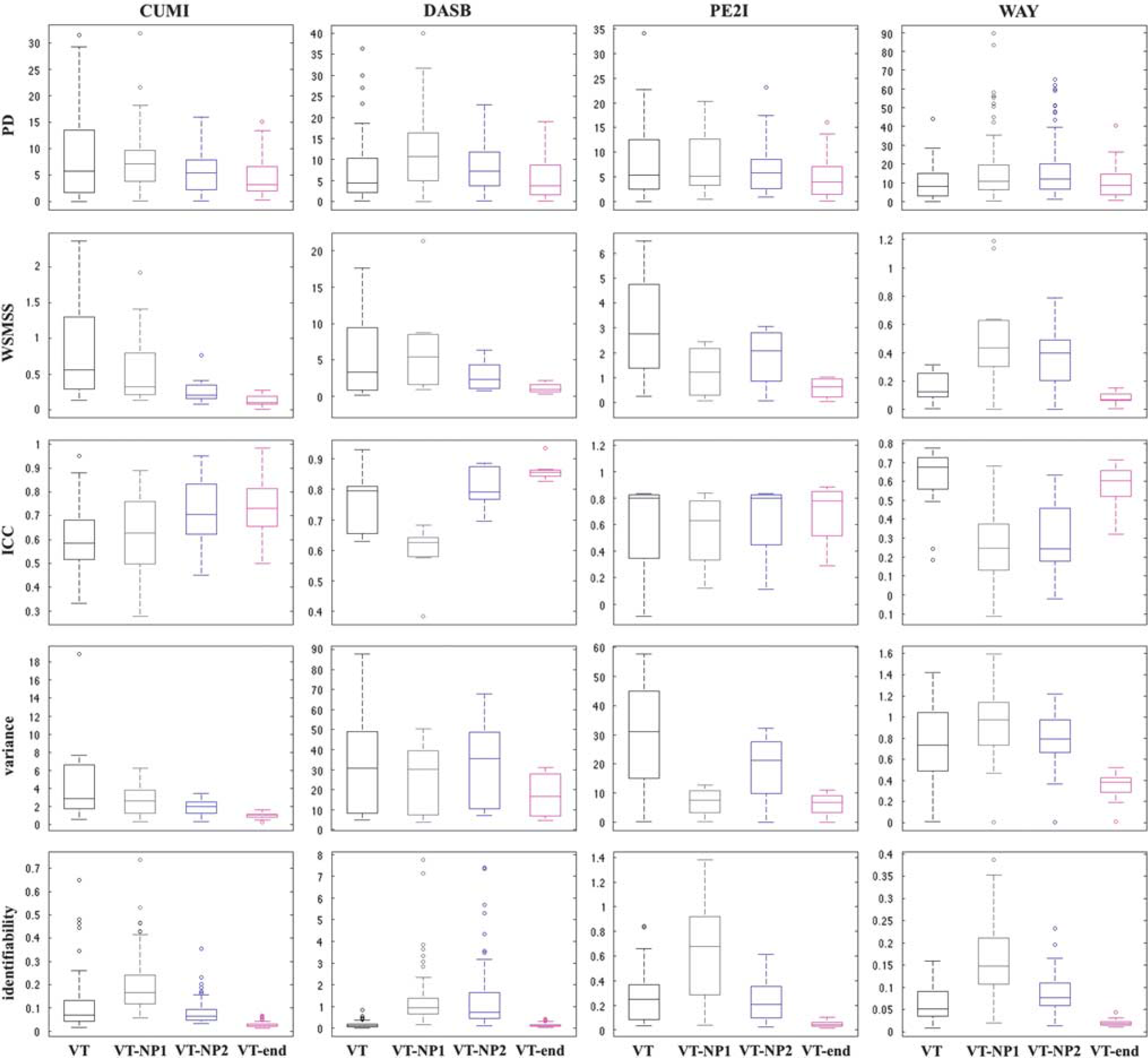
Boxplots of the five considered test–retest metrics for all considered tracers and the four different estimations of the outcome measure (V_T, V_T-NP1, V_T-NP2, V_T-end). In each box, the central mark is the median value of the metric (across subjects/pairs and regions), the edges of the box are the 25th and 75th percentiles, the whiskers extend to the most extreme data points of the metric not considered outliers, and outliers are plotted individually. ICC, interclass correlation coefficient; PD, percent difference; V_T, total volume of distribution; WSMSS, within-subject mean sum of squares.

Figure 4.

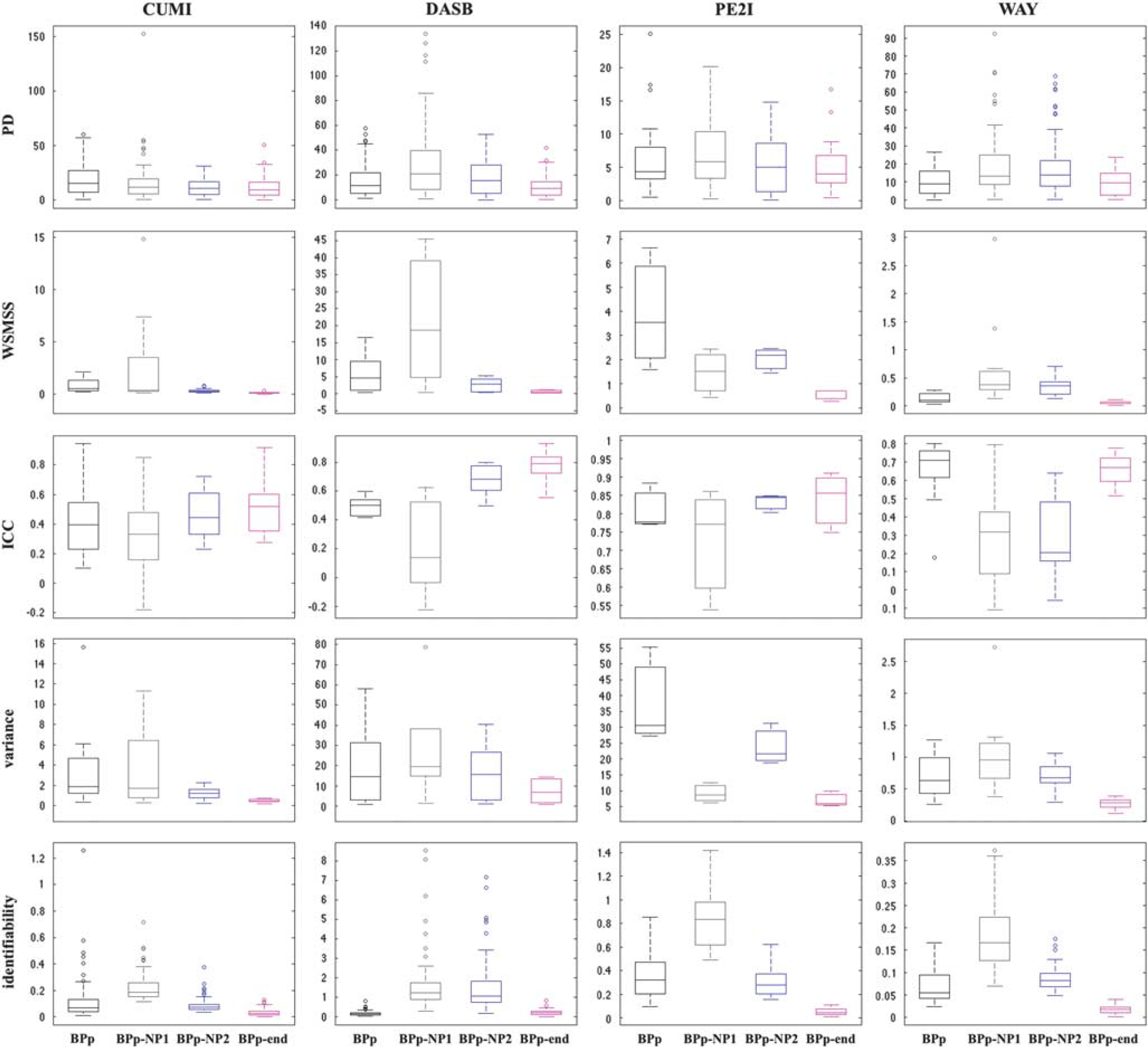
Boxplots of the five considered test–retest metrics for all considered tracers and the four different estimations of the outcome measure (BP_P, BP_P-NP1, BP_P-NP2, BP_P-end). In each box, the central mark is the median value of the metric (across subjects/pairs and regions), the edges of the box are the 25th and 75th percentiles, the whiskers extend to the most extreme data points of the metric not considered outliers, and outliers are plotted individually. BP, binding potential; ICC, interclass correlation coefficient; PD, percent difference; WSMSS, within-subject mean sum of squares.

Table 1 summarizes which outcome measure provides the best performance. For the clinical data, the outcome measures with the best correlation and slope (with the corresponding outcome measures estimated with CMs) are reported separately from the test–retest metrics; the best performance in the test–retest metrics is reported both considering and not considering V_T-end (or BP_P-end).

Table 1

Summary of which outcome measure provides the best performance in each of the simulated and clinical data sets

	Simulated data
	VT			BPp
	Best variance		Best bias	Best variance	Best bias
1TC	VT-end		VT-NP2	BPp-end	BPp-NP2
2TC	VT-end		VT-end	BPp-end	BPp-NP2
Clinical data
	Best correlation		Best slope	Best correlation	Best slope

CUMI	VT-NP2		VT-NP1	BPp-NP2	BPp-NP1
DASB	VT-NP2		VT-NP2	BPp-NP2	BPp-NP2
PE2I	VT-NP2		VT-NP2	BPp-NP2	BPp-NP2
WAY	VT-NP2		VT-NP2	BPp-NP2	BPp-NP2

Test–retest metrics
	PD	WSMSS	ICC	Variance	Identifiability

VT (considering VT-end)
CUMI	VT-end	VT-end	VT-end	VT-end	VT-end
DASB	VT-end	VT-end	VT-end	VT-end	VT-end
PE2I	VT-end	VT-end	VT/VT-NP2	VT-end	VT-end
WAY	VT	VT-end	VT	VT-end	VT-end
VT (not considering VT-end)
CUMI	VT-NP2	VT-NP2	VT-NP2	VT-NP2	VT-NP2
DASB	VT	VT-NP2	VT/VT-NP2	VT-NP1	VT
PE2I	VT-NP1	VT-NP1	VT/VT-NP2	VT-NP1	VT-NP2
WAY	VT	VT	VT	VT	VT
BPp (considering BPp-end)
CUMI	BPp-NP2	BPp-end	BPp-end	BPp-end	BPp-end
DASB	BPp-end	BPp-end	BPp-end	BPp-end	BPp
PE2I	BPp-end	BPp-end	BPp-end	BPp-end	BPp-end
WAY	BPp	BPp-end	BPp	BPp-end	BPp-end
BPp (not considering BPp-end)
CUMI	BPp-NP2	BPp-NP2	BPp-NP2	BPp-NP2	BPp
DASB	BPp	BPp-NP2	BPp-NP2	BPp	BPp
PE2I	BPp	BPp-NP1	BPp-NP2	BPp-NP1	BPp-NP2
WAY	BPp	BPp	BPp	BPp	BPp

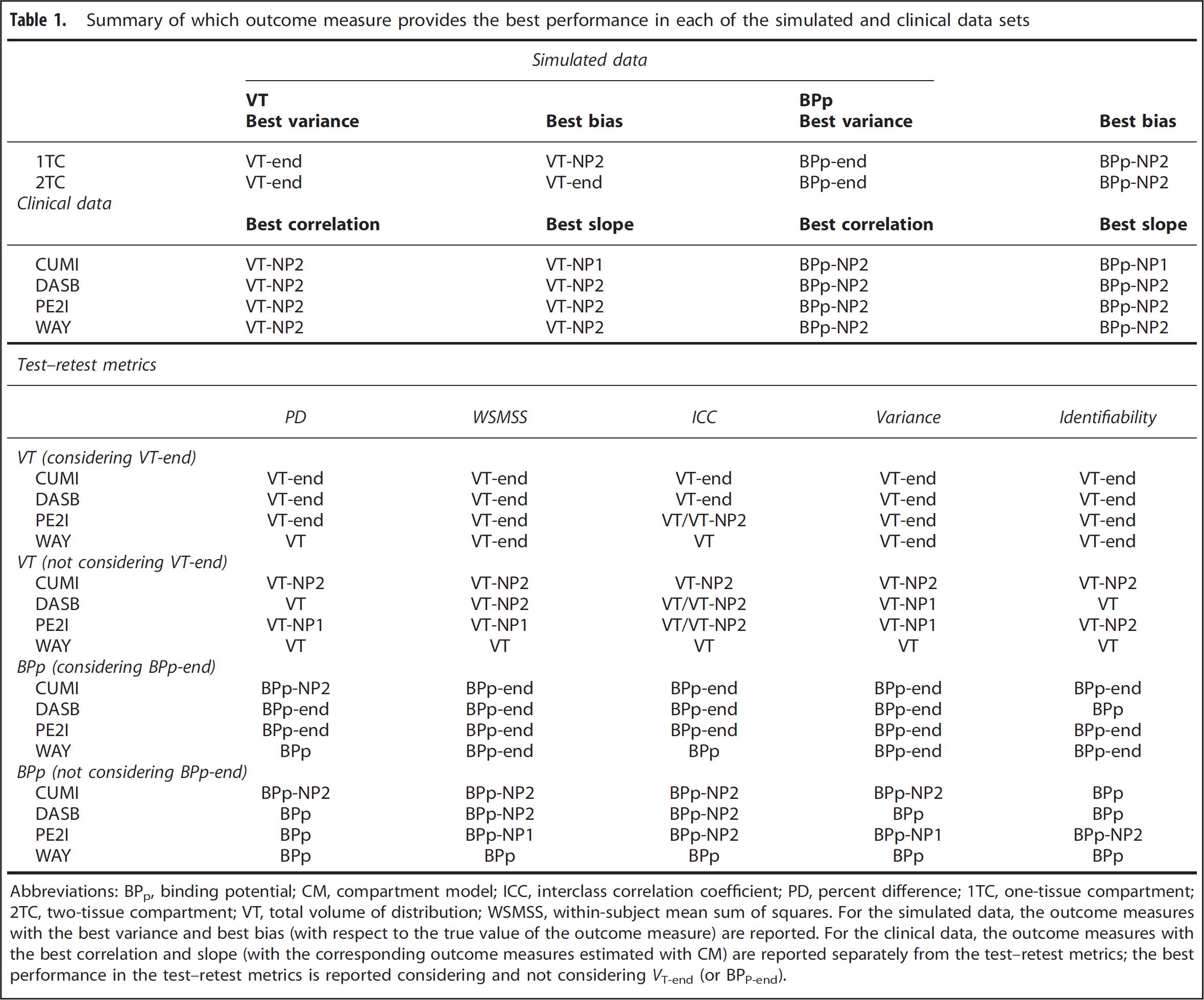
Abbreviations: BP_p, binding potential; CM, compartment model; ICC, interclass correlation coefficient; PD, percent difference; 1TC, one-tissue compartment; 2TC, two-tissue compartment; VT, total volume of distribution; WSMSS, within-subject mean sum of squares.

For the simulated data, the outcome measures with the best variance and best bias (with respect to the true value of the outcome measure) are reported. For the clinical data, the outcome measures with the best correlation and slope (with the corresponding outcome measures estimated with CM) are reported separately from the test–retest metrics; the best performance in the test–retest metrics is reported considering and not considering V_T-end (or BP_P-end).

V_T-end shows the lowest WSMSS and variance, and the best identifiability, for all tracers. V_T-end also shows the lowest PD for CUMI, DASB, and PE2I, and the highest ICC for CUMI and DASB. Correspondingly, BP_P-end shows the lowest WSMSS and variance for all tracers. BP_P-end also shows the highest ICC for all tracers, besides WAY, the lowest PD for DASB and PE2I, and the best identifiability for all tracers, with exclusion of DASB.

V_T and BP_P show the lowest PD and the highest ICC for WAY. BP_P also shows the best identifiability for DASB.

V_T-NP1 and BP_P-NP1 show the worst identifiability for all tracers. BP_P-NP1 also shows the lowest ICC for all tracers, besides WAY.

V_T-NP2 shows the highest ICC for PE2I (0.80), while BP_P-NP2 shows the lowest PD for CUMI.

Simulated Data

Figures 5 and 6 show the distribution of outcome measures obtained using SVD in the 1TCM and 2TCM case, respectively (top panel: V_T-end, V_T-NP1, V_T-NP2; bottom panel: BP_P-end, BP_P-NP1, BP_P-NP2), with simulated noise level corresponding to α = 1. Each region is reported separately (the cerebellum gray matter is the RR for calculation of BP_P-end, BP_P-NP1, BP_P-NP2; therefore, it is not reported for that outcome measure); the dotted vertical lines represent the median of the distribution for each formulation of the outcome measure, while the black solid vertical line represents the true simulated value for that outcome measure and region.

Figure 5.

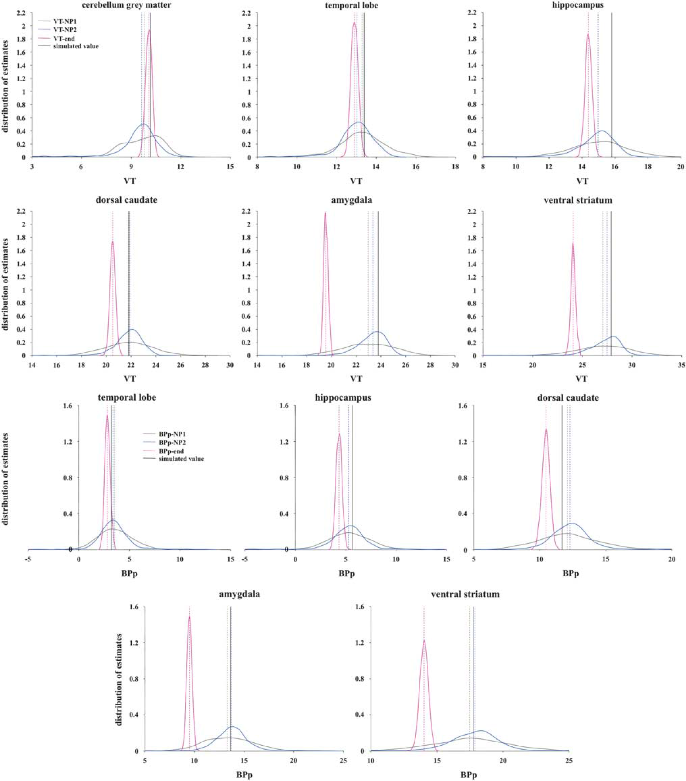
Distribution of outcome measures estimated using singular value decomposition (SVD) and the three nonparametric formulations (top panel: V_T-end, V_T-NP1, V_T-NP2; bottom panel: BP_P-end, BP_P-NP1, BP_P-NP2) across the 1,000 simulated one-tissue compartment model (1TCM) cases in each region; the six simulated regions are reported separately (the cerebellum gray matter is used as the reference region (RR) for the calculation of BP_P-end, BP_P-NP1, BP_P-NP2; therefore, it is not reported for that outcome measure); the dotted vertical lines represent the median of the distribution for each formulation, while the black solid vertical line represents the true simulated value for that outcome measure and region. The data underlying the simulations were derived from clinical [¹¹C]DASB scans modeled with 1TCM. BP_p, binding potential; V_T, total volume of distribution.

Figure 6.

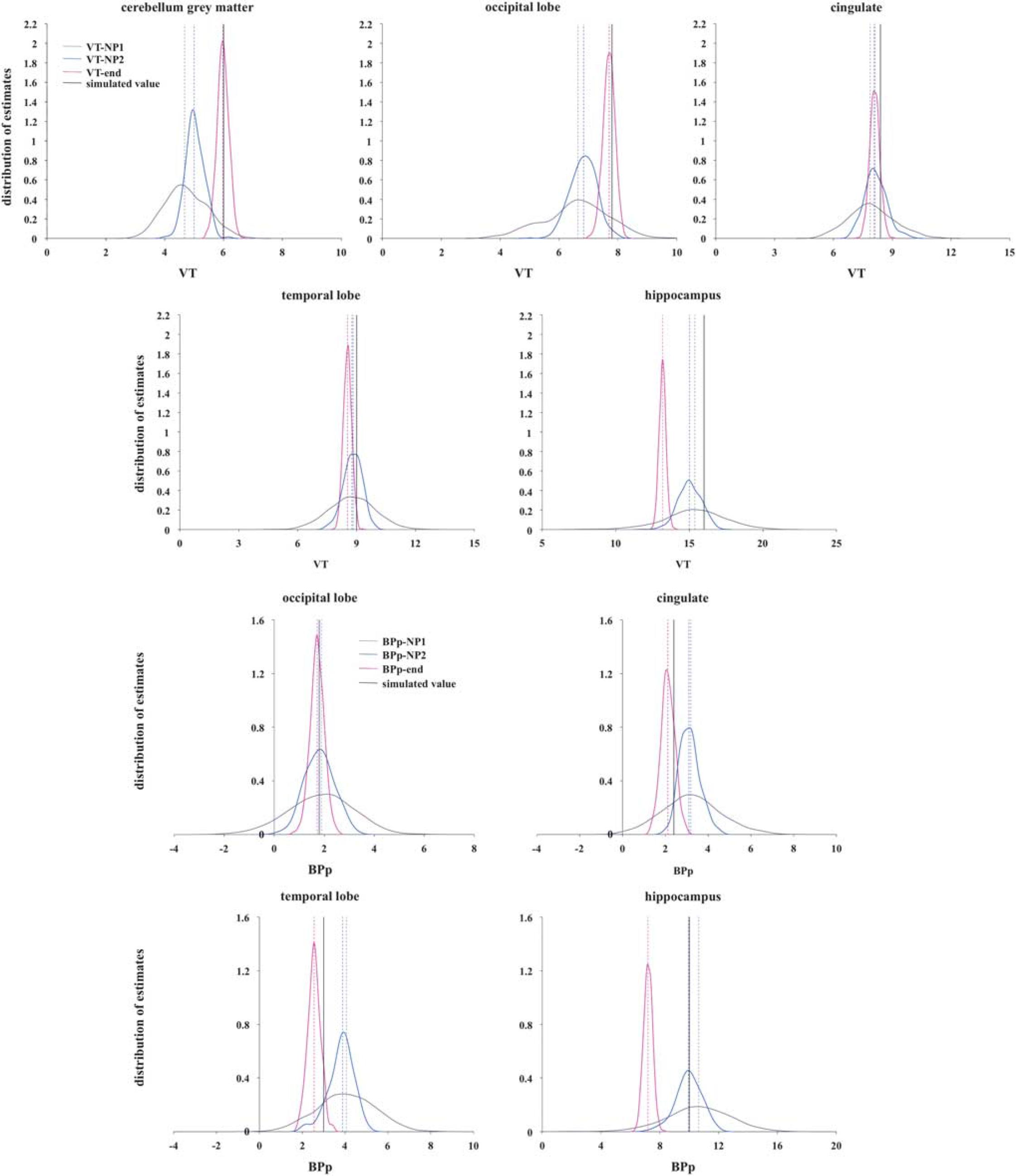
Distribution of outcome measures estimated using singular value decomposition (SVD) and the three nonparametric formulations (top panel: V_T-end, V_T-NP1, V_T-NP2; bottom panel: BP_P-end, BP_P-NP1, BP_P-NP2) across the 1,000 simulated two-tissue compartment model (2TCM) cases in each region; the five simulated regions are reported separately (the cerebellum gray matter is used as the reference region (RR) for the calculation of BP_P-end, BP_P-NP1, BP_P-NP2; therefore, it is not reported for that outcome measure); the dotted vertical lines represent the median of the distribution for each formulation, while the black solid vertical line represents the true simulated value for that outcome measure and region. The data underlying the simulations were derived from clinical [¹¹C]CUMI scans modeled with 2TCM. BP_p, binding potential; V_T, total volume of distribution.

In the 1TCM case, V_T-end always underestimates V_T the most across the three formulations, except for the cerebellum gray matter, although with much less variability. In the 2TCM case, V_T-end performs the best for the three regions with the lowest V_T (cerebellum gray matter, occipital lobe, and cingulate), but underestimates the most the region with the highest V_T (hippocampus). Correspondingly, BP_P-end always underestimates BP_P the most in both cases.

In the 1TCM case, V_T-NP1 and V_T-NP2 show similar median values for V_T, with V_T-NP2 performing better than V_T-NP1 for the three regions with highest simulated V_T (dorsal caudate, amydgala, ventral striatum). In the 2TCM case, it is V_T-NP1 that slightly outperforms V_T-NP2 in all regions in terms of bias, but not variance of the estimates distribution. Corresponding BP_P-NP1 and BP_P-NP2 values are similar in the 1TCM case, while BP_P-NP1 tends to overestimate the BP_P in all the regions in the 2TCM case. BP_P-NP2 shows the smallest bias across regions and less dispersed distributions than the ones of BP_P-NP1 in the 2TCM case.

As reported in Table 1, with the noise present at the ROI level (α = 1), V_T-end and BP_P-end show the best variance in both simulated cases: 0.039 and 0.084 (1TCM); 0.043 and 0.090 (2TCM). V_T-end shows the smallest bias (–0.298) for 2TCM, while V_T-NP2 shows the smallest bias for 1TCM (–0.426), and BP_P-NP2 shows the smallest bias for both 1TCM (0.129) and 2TCM (0.351).

The results relative to the noise analysis are reported in the Supplementary Material. In both 1TCM and 2TCM cases, the bias of the V_T-end and BP_P-end estimates is almost constant across the five noise conditions. The corresponding variance, although it increases with the noise in the data, remains significantly lower than the corresponding variance of the other two nonparametric formulations for the same outcome measure.

In both 1TCM and 2TCM cases, the pattern with which the bias of V_T-NP1 and BP_P-NP1, and V_T-NP2 and BP_P-NP2, changes with noise is similar, with both formulations that tend to overestimate the true value at elevated noise levels. In the 1TCM case, the bias of V_T-NP2 and BP_P-NP2 increases the most with the noise level. The corresponding variance values increase with noise, with V_T-NP1 and BP_P-NP1 providing the worst performance in the 2TCM case. In the 1TCM case, the variance of V_T-NP1 and V_T-NP2, and BP_P-NP1 and BP_P-NP2, is almost identical.

DISCUSSION

We applied nonparametric deconvolution to estimate the IRF of PET reversible tracers in several regions, using both simulated and clinical test–retest data sets, computed several functionals of the IRF to estimate tracer V_T and BPs, and extensively compared these functionals with traditional outcome measures derived using CMs. We showed that nonparametric deconvolution, which does not require any model assumptions, and the functionals that can be computed from the recovered IRF can provide estimates of V_T and BP_P that are not only very close to, and highly correlated with, the estimated obtained with traditional CMs, but can also show better test–retest performance than outcome measures derived from CMs. Therefore, nonparametric deconvolution and the proposed functionals offer a promising alternative to CMs for the quantification of PET dynamic data, especially when CMs assumptions do not hold or when CMs provide poor fits and/or unphysiologic estimates of the outcome measures for a specific PET tracer.

The optimized formulation of V_T we proposed in Equation (10), and the corresponding BP_P-NP2 that can be derived, provide the best performance in terms of bias with respect to, and correlation with, outcome measures with traditional CMs in the majority of the simulated and clinical considered data sets (Table 1). V_T-end as in Equation (8), and the corresponding BP_P-end that can be derived, provide the best test–retest performance across metrics and, overall, considered tracers; outcome measures derived with traditional CMs show superior test–retest performance than V_T-end and BP_P-end only for some of the metrics in the case of DASB (identifiability of BP_P), PE2I (ICC of V_T), and WAY (PD and ICC of V_T and BP_P). Therefore, V_T-end and BP_P-end are stable (with respect to noise in the TACs) and reliable outcome measures that could be used, for example, to discriminate different clinical populations from each other and from healthy controls. However, as one would expect from their definitions, results on simulated and clinical data sets suggest that V_T-end and BP_P-end often provide the greatest underestimation of V_T and BP_P (with the exception of PE2I BP_P, for which BP_P-NP1 shows the greatest underestimation). This is perhaps less of an issue if the purpose of the study is to examine differences between groups (or across values of some continuous variable) but if the primary goal of the analysis is estimation of standard outcome measures, the bias of these estimates must be considered. In such a situation, V_T-NP1 and/or V_T-NP2 (and the corresponding BP_P-NP1 and BP_P-NP2) could be considered, as they show better test–retest performance than CMs outcomes according to the majority of the considered metrics for all tracers, with the exception of WAY.

An intrinsic limitation of the nonparametric approach is that the IRF can be estimated only up to the end of the PET scan, and no inference up to infinity can therefore be made without some strong assumptions. For example, it may be the case that, for tracers that slowly reach equilibrium, the nonparametric estimation of V_T and BP_P according to equations (9 and 10) is biased by the fact that, by the end of the scan, the IRF has not yet reached a certain fraction of its initial value, and therefore the corresponding k^th quantile of the residence cannot be determined. Estimation of V_T-end and BP_P-end instead might be preferred in these cases, with proper interpretation of the results.

We have implemented here nonparametric deconvolution using SVD^9,10 with an automatic data-driven selection of the threshold for each ROI. This is a fast, easy to implement, and widely adopted approach to deconvolution that easily lends itself to implementation at the voxel level. However, we claim no optimality in either the choice of the deconvolution approach or the selection of the thresholds.

It is known that SVD performance can be sensitive to the level of the noise present in the data.^27,28 Our simulation results at different noise level (see Supplementary material) suggest that, at the voxel level, or for particularly noisy tracers, either V_T-end and BP_P-end should be preferred as outcome measures because they are less affected by noise, or more robust approaches to deconvolution, such as nonlinear stochastic regularization²⁸ or kernel-based linear system identification,^29,30 should be considered for reconstructing the IRF.

The cross-validation algorithm we propose here for thresholding the singular values in the decomposition to constrain the propagation of noise from the data to the IRF estimates is data driven and has proven to be flexible enough to provide reasonably regularized solutions for the considered four tracers and simulated data. However, other strategies exist,^7,31–33 which may provide improved solutions. The optimization of the thresholding algorithm, which likely depends on the tracer at hand, is however beyond the scope of this article.

Singular value decomposition, as many other nonparametric deconvolution approaches, requires the input data to be equidistantly sampled.²³ The PET data involve radioactive decay, and are usually acquired using increasing frame lengths to ensure a comparable number of counts and thus statistical quality per data point. This implies that the PET data need to be interpolated on an equally-spaced grid of temporal values before applying SVD. The possible effect of the interpolation on the estimation of V_T and BP_P should be further investigated, especially when using SVD at the voxel level where, due to the large number of voxels to quantify, adopting a very fine interpolation grid can lead to out-of-memory issues during the quantification process. While Shannon's sampling theorem²³ implies that any band-limited signal can be reconstructed from its regularly spaced samples, the solution of the nonuniform sampling problem poses more difficulties.²⁴ There exist a vast literature on nonuniform sampling theory^34,35 and methods claiming to efficiently reconstruct a function from its nonuniform samples,^36–38 including nonuniform SVD.³⁹ The investigation of the performance on PET data of nonuniform deconvolution approaches is however beyond the scope of this article.

It is important to state that comparing the performance of the proposed nonparametric outcome measures with the corresponding CMs estimates is not generally useful when the CM is not valid for the tracer in question. Here, we have considered four tracers for which we have already assessed the validity of the CMs,^14–17 so the proposed comparison is meaningful, although it may be questioned in certain individual regions. Certainly, the possibility of quantifying the binding of PET tracers model-free and nonparametrically is particularly attractive for those tracers for which the assumptions of CMs do not hold or CMs do not provide a good description of the data. In these cases, however, the CMs estimates of the binding cannot be used as a reference to evaluate the performance of the nonparametric approach, and validation with in vitro results would be recommended.

Future directions of investigation also include the extension of the presented nonparametric approach to quantification in the absence of a metabolite-corrected input function.

CONCLUSIONS

Nonparametric deconvolution does not require any model assumptions and allows for estimates of V_T and BP_P that are very close to the estimates obtained with traditional CMs, and can also show superior test–retest performance. Nonparametric deconvolution and the proposed functionals therefore offer a viable alternative to CMs for the quantification of PET dynamic data, especially when CMs assumptions do not hold or CMs provide poor fits and/or unphysiologic estimates of the outcome measures for a specific PET tracer.

AUTHOR CONTRIBUTIONS

Dr Zanderigo was responsible for ideation of the methodologies, drafting of the manuscript, creation of the software, analysis and interpretation of the data. Dr Parsey contributed to conception and revision of the manuscript, and interpretation of the data. Dr Ogden contributed to ideation of the methodologies, interpretation of the data, critical revision of the manuscript, and final approval.

DISCLOSURE/CONFLICT OF INTEREST

The authors declare no conflict of interest.

Footnotes

Notes

Supplementary Information accompanies the paper on the Journal of Cerebral Blood Flow & Metabolism website ()

References

Innis

Cunningham

Delforge

Fujita

Gjedde

Gunn

Consensus nomenclature for in vivo imaging of reversibly binding radioligands. J Cereb Blood Flow Metab 2007; 27: 1533–1539.

Slifstein

Laruelle

. Models and methods for derivation of in vivo neuroreceptor parameters with PET and SPECT reversible radiotracers. Nucl Med Biol 2001; 28: 595–608.

O'Sullivan

Muzi

Spence

Mankoff

O'Sullivan

Fitzgerald

Nonparametric residue analysis of dynamic PET data with application to cerebral FDG studies in normals. J Am Stat Assoc 2009; 104: 556–571.

Jiang

C-R

Aston

JAD

Wang

J-L

. A functional approach to deconvolve dynamic neuroimaging data 2014; arXiv.org/stat/arXiv:1411.2051.

Cunningham

Jones

. Spectral analysis of dynamic PET studies. J Cereb Blood Flow Metab 1993; 13: 15–23.

Gunn

Turkheimer

Aston

Cunningham

. Positron emission tomography compartmental models: a basis pursuit strategy for kinetic modeling. J Cereb Blood Flow Metab 2002; 22: 1425–1439.

Turkheimer

Hinz

Gunn

Aston

Gunn

Cunningham

. Rank-shaping regularization of exponential spectral analysis for application to functional parametric mapping. Phys Med Biol 2003; 48: 3819–3841.

Schmidt

. Which linear compartmental systems can be analyzed by spectral analysis of PET output data summed over all compartments? J Cereb Blood Flow Metab 1999; 19: 560–569.

Ostergaard

Weisskoff

Chesler

Gyldensted

Rosen

. High resolution measurement of cerebral blood flow using intravascular tracer bolus passages. Part I: Mathematical approach and statistical analysis. Magn Reson Med 1996; 36: 715–725.

10.

Ostergaard

Sorensen

Kwong

Weisskoff

Gyldensted

Rosen

. High resolution measurement of cerebral blood flow using intravascular tracer bolus passages. Part II: Experimental comparison and preliminary results. Magn Reson Med 1996; 36: 726–736.

11.

Buchert

Wilke

Van den Hoff

Mester

. Improved statistical power of the multilinear reference tissue approach to the quantification of neuroreceptor ligand binding by regularization. J Cereb Blood Flow Metab 2003; 23: 612–620.

12.

Constantinescu

Bouman

Morris

. Nonparametric extraction of transient changes in neurotransmitter concentration from dynamic PET data. IEEE Trans Med Imaging 2007; 26: 359–373.

13.

Grecchi

Doyle

Bertoldo

Pavese

Turkheimer

. Brain shaving: adaptive detection for brain PET data. Phys Med Biol 2014; 59: 2517–2534.

14.

Milak

DeLorenzo

Zanderigo

Prabhakaran

Kumar

Majo

In vivo quantification of human serotonin 1A receptor using 11C-CUMI-101, an agonist PET radiotracer. J Nucl Med 2010; 51: 1892–1900.

15.

Ogden

Ojha

Erlandsson

Oquendo

Mann

Parsey

. In vivo quantification of serotonin transporters using [(11)C]DASB and positron emission tomography in humans: modeling considerations. J Cereb Blood Flow Metab 2007; 27: 205–217.

16.

DeLorenzo

Kumar

Zanderigo

Mann

Parsey

. Modeling considerations for in vivo quantification of the dopamine transporter using [(11)C]PE2I and positron emission tomography. J Cereb Blood Flow Metab 2009; 29: 1332–1345.

17.

Parsey

Slifstein

Hwang

Abi-Dargham

Simpson

Mawlawi

Validation and reproducibility of measurement of 5-HT1A receptor parameters with [carbonyl-11C]WAY-100635 in humans: comparison of arterial and reference tisssue input functions. J Cereb Blood Flow Metab 2000; 20: 1111–1133.

18.

Jenkinson

Smith

. A global optimisation method for robust affine registration of brain images. Med Image Anal 2001; 5: 143–156.

19.

Smith

. Fast robust automated brain extraction. Hum Brain Mapp 2002; 17: 143–155.

20.

Parsey

Ogden

Mann

. Determination of volume of distribution using likelihood estimation in graphical analysis: elimination of estimation bias. J Cereb Blood Flow Metab 2003; 23: 1471–1478.

21.

Parsey

Ojha

Ogden

Erlandsson

Kumar

Landgrebe

Metabolite considerations in the in vivo quantification of serotonin transporters using 11C-DASB and PET in humans. J Nucl Med 2006; 47: 1796–1802.

22.

Meier

Zierler

. On the theory of the indicator-dilution method for measurement of blood flow and volume. J Appl Physiol 1954; 6: 731–744.

23.

Shannon

. A mathematical theory of communication. Bell Syst Tech J 1948; 27: 379–623.

24.

Strohmer

. Numerical analysis of the non-uniform sampling problem. J Comput Appl Math 2000; 122: 297–316.

25.

Press

Teukolsky

Vetterling

Flannery

. Numerical Recipes in C. 2nd edition Cambridge University Press: Oxford, 1992.

26.

Ogden

Tarpey

. Estimation in regression models with externally estimated parameters. Biostatistics 2006; 7: 115–129.

27.

Knutsson

Stahlberg

Wirestam

. Aspects on the accuracy of cerebral perfusion parameters obtained by dynamic susceptibility contrast MRI: a simulation study. Magn Reson Imaging 2004; 22: 789–798.

28.

Zanderigo

Bertoldo

Pillonetto

Cobelli Ast

. Nonlinear stochastic regularization to characterize tissue residue function in bolus-tracking MRI: assessment and comparison with SVD, block-circulant SVD, and Tikhonov. IEEE Trans Biomed Eng 2009; 56: 1287–1297.

29.

Pillonetto

. DNG. A new kernel-based approach for linear system identification. Automatica 2010; 46: 81–93.

30.

Castellaro

Peruzzo

Mehndiratta

Pillonetto

Petersen

Golay

Estimation of arterial arrival time and cerebral blood flow from QUASAR arterial spin labeling using stable spline. Magn Reson Med 2014; doi: 10.1002/mrm.25525 (e-pub ahead of print).

31.

Murase

Yamazaki

Miyazaki

. Deconvolution analysis of dynamic contrast-enhanced data based on singular value decomposition optimized by generalized cross validation. Magn Reson Med Sci 2004; 3: 165–175.

32.

Sourbron

Luypaert

Van Schuerbeek

Dujardin

Stadnik

. Choice of the regularization parameter for perfusion quantification with MRI. Phys Med Biol 2004; 49: 3307–3324.

33.

Liu

Nickerson

Andrews

Fox

Cerebral blood flow measurement by dynamic contrast MRI using singular value decomposition with an adaptive threshold. Magn Reson Med 1999; 42: 167–172.

34.

Landau

. Necessary density conditions for sampling and interpolation of certain entire functions. Acta Math 1967; 117: 37–52.

35.

Feichtinger

Gröchenig

. Theory and practice of irregular sampling. Benedetto

Frazier

, (Eds.), Wavelets: Mathematics and Applications. CRC Press: Boca Raton, FL, 1994; 305–363.

36.

Yao

K TJ

. On some stability and interpolatory properties of nonuniform sampling expansions. IEEE Trans Circuit Theory 1967; 14: 404–408.

37.

Feichtinger

HG GK

Strohmer

. Efficient numerical methods in non-uniform sampling theory. Numer Math 1995; 69: 423–440.

38.

De Nicolao

Liberati

Sartorio

. Deconvolution of infrequently sampled data for the estimation of growth hormone secretion. IEEE Trans Biomed Eng 1995; 42: 678–687.

39.

Wingham

. The reconstruction of a band-limited function and its Fourier transform from a finite number of samples at arbitrary locations by singular value decomposition. IEEE Trans Circuit Theory 1967; 40: 559–570.

Supplementary Material

Please find the following supplemental material available below.

For Open Access articles published under a Creative Commons License, all supplemental material carries the same license as the article it is associated with.

For non-Open Access articles published, all supplemental material carries a non-exclusive license, and permission requests for re-use of supplemental material or any part of supplemental material shall be sent directly to the copyright owner as specified in the copyright notice associated with the article.

0.00 MB

0.92 MB

Model-Free Quantification of Dynamic PET Data Using Nonparametric Deconvolution

Abstract

Keywords

INTRODUCTION

MATERIALS AND METHODS

SUBJECTS

Positron Emission Tomography Protocol

Image Analysis

Simulated Data

Interpretation of Positron Emission Tomography Data

Outcome Measures

Singular Value Decomposition

Metrics of Comparison for Simulated Data

Application to Test–Retest Data

RESULTS

Test–Retest Data

Simulated Data

DISCUSSION

CONCLUSIONS

AUTHOR CONTRIBUTIONS

DISCLOSURE/CONFLICT OF INTEREST

Footnotes

Notes

References

Supplementary Material