The Influence of Noise on Bold-Mediated Vessel Size Imaging Analysis Methods

Abstract

Vessel size imaging (VSI) is a magnetic resonance imaging (MRI) technique that aims to provide quantitative measurements of tissue microvasculature. An emerging variation of this technique uses the blood oxygenation level-dependent (BOLD) effect as the source of the imaging contrast. Gas challenges have the advantage over contrast injection techniques in that they are noninvasive and easily repeatable because of the fast washout of the contrast. However, initial results from BOLD-VSI studies are somewhat contradictory, with substantially different estimates of the mean vessel radius. Owing to BOLD-VSI being an emerging technique, there is not yet a standard processing methodology, and different techniques have been used to calculate the mean vessel radius and reject uncertain estimates. In addition, the acquisition methodology and signal modeling vary from group to group. Owing to these differences, it is difficult to determine the source of this variation. Here we use computer modeling to assess the impact of noise on the accuracy and precision of different BOLD-VSI calculations. Our results show both potential overestimates and underestimates of the mean vessel radius, which is confirmed with a validation study at 3T.

INTRODUCTION

Magnetic resonance imaging (MRI) measurement of vessel size aims to provide a quantitative measurement of tissue microvasculature. Typically, the mean vessel size, or vessel caliber index (VCI), is calculated from the ratio of the change in R₂∗ and R₂ because of the injection of a contrast agent.^{1, 2, 3} In the majority of studies either gadolinium diethylenetriaminepenta-acetic acid (Gd-DTPA) or superparamagnetic iron oxide particles are used as the contrast agent. Alternatively, the blood oxygenation level-dependent (BOLD) effect can be used as the source of this contrast.^{4, 5, 6, 7} The blood oxygenation is modulated with either hypoxic, hyperoxic, or hypercapnic gas challenges, probing the venous vasculature.

The use of contrast agents to determine the mean vessel size has been validated with histology in a number of animal studies.^{1, 8, 9, 10} For example, Lemasson et al ¹⁰ found a high correlation between VCI and stereologic measurements on histology data from rat brain tumor and Bosomtwi et al ⁸ showed a significant correlation between MRI-derived vessel size and histologic measurement after stroke. In addition, clinical studies have shown the potential of vessel size imaging (VSI) to provide a noninvasive assessment of tumor grade ¹¹ and aid in defining the ischemic penumbra in acute stroke. ¹² Although the initial clinical findings are promising, the requirement to inject a contrast agent somewhat limits the potential patient population. Furthermore, because of the requirement of paramagnetic contrast agents to remain intravascular the technique is limited to the brain, where the blood–brain barrier restricts the distribution of the contrast agent to the intravascular space. ⁶

To date a small number of BOLD-VSI studies have been reported in the literature. The first quantitative study ¹³ used blocks of visual stimulation to modulate the BOLD signal, whereas subsequent studies^{4, 6, 7} have used gas challenges. Some difference between BOLD-VSI and Gd-DTPA studies might be expected; with Gd-DTPA providing contrast to the whole vascular system while BOLD provides a venous weighted contrast. However, there is a degree of symmetry between the arterial and venous vasculature. In vivo measurements show that the average cerebral arteriole and venule radii are approximately the same, 26.5 and 25.5 μm, respectively. ¹⁴ Therefore, we might expect the measured VSI distributions to be similar. Indeed, initial BOLD-VSI experiments^{4, 13} do show a high degree of similarity with Gd-DTPA measurements.^{12, 15, 16} However, subsequent BOLD-VSI measurements^{6, 7} estimate a mean vessel radius that is <50% of these. The difference in vessel size estimates appear to derive primarily from a difference in the measured ΔR₂∗/ ΔR₂ ratio (denoted q). Although changes in q might be expected with field strength, the signal modeling used for VCI calculations is expected to account for this. Such large differences in vessel size estimates need to be addressed before BOLD-VSI can be considered a robust and reliable technique, suitable for clinical implementation.

As the BOLD signal provides a relatively low contrast-to-noise (CNR) measurement, BOLD-VSI is inherently more sensitive to noise than contrast-based methods. We believe it is this noise sensitivity that underlies some of the discrepancy in vessel size estimates obtained with this technique. Here we use computer modeling to assess the impact of noise on the accuracy q and VCI calculations with different BOLD-VSI analysis methods and noise content. The results of the modeling are then compared with in vivo measurements using an oxygen challenge and different levels of spatial smoothing, producing a number of data sets with varying CNR.

MATERIALS AND METHODS

Signal Modeling

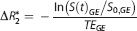
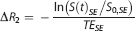
The magnitude of MRI signals acquired with gradient echo (GE) and spin echo (SE) acquisitions are dependent on the transverse relaxation rates R₂ ^∗ and R₂, respectively. Assuming monoexponential signal decay, constant proton density and negligible T₁ effects (related to inflow or molecular oxygen), changes in transverse relaxation rates can be determined from GE and SE acquisitions as per equations (1a and 1b).

$\mathrm{\Delta }{R}_2^{\ast }=-\frac{\text{ln}(S(t{)}_{GE}∕S_{0,GE})}{T{E}_{GE}}$

(1a)

$\mathrm{\Delta }{R}_2=-\frac{\text{ln}(S(t{)}_{SE}∕S_{0,SE})}{T{E}_{SE}}$

(1b)

Where S(t) is the time course of the signal magnitude, S₀ is its average value during baseline and TE is the corresponding GE or SE time.

As ΔR₂∗ and ΔR₂ have differential vessel size sensitivity, ¹⁷ the vessel radius, r_v, can be modeled as a function of q and the BOLD-induced susceptibility change, Δχ, ⁴ so that r_v=f(q,Δχ). Therefore, by acquiring GE and SE signals during rest and stimulation, estimates of the vessel radius can be made. In vivo, each voxel will typically contain a distribution of vessel radii. If this distribution has a small variance compared with the mean, then the measured q (and therefore r_v) will be equal to the mean. ¹³ Given this, r_v represents the voxelwise average over the postcapillary population with each vessel size weighted by its blood volume fraction.

GE and SE signals (at 3T and 7T) were estimated using a Monte–Carlo simulation of water in a vascular network. The ODIN framework ¹⁸ was used to produce numerical integrations of the Bloch equations along a large number of random walk paths, as described by Jochimsen et al. ¹³ Intravascular signal was also included in the modeling, with the field distribution inside a vessel calculated according to Bandettini and Wong. ¹⁹ Vessel modeling was undertaken for intravascular susceptibility changes, Δχ, ranging from −0.05 to −0.3 p.p.m. (SI units). This range of susceptibility changes was chosen to include the measured susceptibility change with oxygen in volunteers and the reported susceptibility changes in previous studies.

In all simulations, the difference between fully oxygenated and deoxygenated hemoglobin was taken to be 0.264 p.p.m. ²⁰ A diffusion coefficient of 0.76 × 10⁻³ mm²/second, a postcapillary blood volume fraction of 3%, and a hematocrit of 0.40 were assumed. GE and SE echo times of 30/90 milliseconds at 3T and 18/55 milliseconds at 7T were chosen to be representative of recent BOLD-VSI studies. The blood T₂ values at 3T were calculated by fitting to Zhao et al ²¹ and assuming a venous oxy-hemoglobin saturation, Y, of 60% at rest; producing T₂ estimates of 32.2, 36.5, 41.4, 53.3, and 68.0 milliseconds for Δχ=0, −0.05, −0.1, −0.2, and −0.3 p.p.m., respectively. Blood T₂ values at 7T were extrapolated as per Jochimsen et al; ⁴ producing T₂ estimates of 8.1, 9.7, 12.0, 18.4, and 27.3 milliseconds for Δχ=0, −0.05, −0.1, −0.2, and −0.3 p.p.m., respectively. Figures 1A and 1B, show plots of VCI against q for the simulated susceptibility changes at 3T and 7T, respectively. It is clear from the figures that the relationship between q and r_v has a much greater dependence on Δχ at 3T compared with 7T (particularly for large q). This is the result of increased sensitivity to intravascular contributions at 3T, which are significantly reduced at 7T because of the short T₂ of blood.

Figure 1.

Modeled relationship between mean vessel radius (μm) and the vessel size index, q. Modeled at 3T (A) and 7T (B) for susceptibility changes −0.05 to −0.3 p.p.m.

It should be noted that the modeling does not account for changes in blood flow or blood volume during stimulation, which are expected in hypercapnic gas challenges. ²² Simulations performed by Shen et al ⁷ suggest only a small error is introduced by ignoring ΔCBV up to 12%. Using a large hypercapnic stimulus, 7% CO₂, Ito et al ²² measured a 30.5% increase in cerebral blood flow with an associated 9.6% change in total blood volume, well below the modeled ΔCBV. Animal experiments ²³ indicate that the venous ΔCBV, which is relevant for BOLD-weighted studies, only accounts for 36% of this increase. However, the majority of this increase occurs in the small cerebral vessels, 5 to 15 μm radius, and was found to be as large as 23% in this range of vessels with a 9% CO₂ stimulus in rat. ²³

Noise Modeling

Magnetic resonance imaging experiments were simulated with MATLAB (Mathworks, Natick, MA, USA) to assess the impact of noise on different analysis methods. The noise modeling used a hybrid simulation, with measured noise added to simulated MR signals. A hybrid simulation method was used to accurately capture the noise characteristics, including any correlation between the GE and SE noise that might arise because of physiologic fluctuations. Noise data sets (n=4) were acquired with Siemens MRI Scanners (Erlangen, Germany) at 3T (Siemens Verio with 32-channel head coil) and 7T (Siemens Magnetom with 32-channel Nova Medical head coil) using identical acquisition parameters to the simulated vessel data, echo time (TE) 30/90 milliseconds at 3T and 18/55 milliseconds at 7T, repetition time (TR) 3.5 seconds. In each case, a GRAPPA acceleration factor of 2 and a matrix size of 64 × 64 was used with a 200 mm field of view. A slice thickness of 3 mm (1 mm slice gap) and 28 slices (26 slices at 7T) were used for full brain coverage.

The measured noise data sets were preprocessed with FSL (FEAT) (http://www.fmrib.ox.ac.uk/fsl). ²⁴ Each data set was registered to a corresponding structural acquisition, corrected for motion, high pass filtered to remove baseline drift (cutoff=400 seconds) and spatially smoothed. For each acquisition, four different data sets were produced with 0, 4, 6, and 8 mm full width at half maximum (FWHM) spatial smoothing. After preprocessing with FEAT, the data sets were masked to produce gray matter volumes, creating over 25,000 GE and SE time courses for each field strength and level of smoothing. Before spatial smoothing, gray matter voxels had a mean time course signal-to-noise ratio (tSNR) of 66±29 for GE acquisitions and 35±13 for SE acquisitions at 3T. At 7T, the GE acquisitions had a similar tSNR, with a mean value of 67±29. However, the SE tSNR value increased slightly to 45±19. Given the nonuniform distribution of tSNR values across the brain, a random sampling of voxels (from all volunteers) was used during simulations, ensuring an unbiased noise distribution for each simulated vessel size.

During modeling, the randomly selected GE and SE noise pairs were added to simulated experimental data, representing the expected BOLD signal change because of a gas challenge. The experimental paradigm consisted of two stimulation blocks of 3 minutes (TR=3.5 seconds) interleaved with three 2-minute baseline periods. When presented with a block gas challenge, the change in oxy-hemoglobin saturation is somewhat delayed and dispersed. To account for this, the block design was convolved with a gamma-variate function (mean lag 30 seconds and s.d. 30 seconds). In our experience, the resulting time course fits well with gray matter BOLD data acquired in CO₂ challenges. Although the mean lag would be greater for an oxygen challenge, which is typically accounted for by longer rest periods, these differences are not expected to have a large influence on the analysis.

Vessel Population Modeling

To analyze the impact of noise when assessing a region of interest, smoothing splines were fitted to the modeled MRI signals, allowing noise simulations to be performed on a distribution of vessel radii between 1 and 70 μm. An assumed VCI distribution was used to modulate the number of simulations at each vessel size (using a step size of 0.01 μm), with a minimum of one simulation at each radius. To extend the range of SNR values probed by the simulations each analysis was repeated using four different levels of spatial noise smoothing (0, 4, 6, and 8 mm FWHM).

The VCI distribution was chosen to represent the expected distribution of mean vessel radii present in gray matter region of interest analysis. The in vivo distribution of the VCI over a region of interest is unknown and cannot easily be inferred from ex vivo measurements, such as confocal laser microscopy. Ex vivo measurements of vessel size typically exclude veins and arteries, and are subject to ill-defined vessel shrinkage; while BOLD-VSI is sensitive to the entire postcapillary network including veins. As such, estimates made using VSI are expected to be significantly greater than ex vivo measurements.

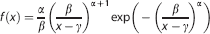
As a result of the difficulty in inferring the true in vivo distribution, we have taken the practical approach in deriving a distribution from the current VSI literature^{4, 12, 13, 15, 16}; which all present data with similar mean values and distributions. However, the Gd-DTPA studies are sensitive to the entire vasculature, not just the postcapillary network. In addition, contrast agent-based experiments have been shown to have a dependence on the relative arterial and venous blood volume and the tracer bolus dispersion. ²⁵ Jochimsen and Moller ¹³ acquired data using a smaller susceptibility change and lower field strength than Jochimsen et al, ⁴ and so are expected to have a lower CNR. As a result of these considerations, the volunteer data presented in (ref. 4) was used as the basis for the VCI distribution. MATLAB was used to fit the averaged data with a generalized extreme value distribution, the resulting probability density function being described by a Frechet distribution (α=0.41, β=5.8, γ=10.1, and R²=0.99), equation (2).

$f(x)=\frac{\alpha }{\beta }{\left(\frac{\beta }{x-\gamma }\right)}^{\alpha +1}\text{exp}(-{\left(\frac{\beta }{x-\gamma }\right)}^{\alpha })$

(2)

Where α is the shape parameter, β is the scale parameter, and γ is the location parameter.

MRI Validation Study

To validate the simulation results, five VSI data sets were acquired at 3T from five healthy volunteers (4 men and 1 woman, mean age 34). The experimental paradigm and data acquisition were identical to the simulations; TR=3.5 TE=30/90 milliseconds, 3 × 3 × 3 mm³ voxel, 28 slices with 1 mm slice gap. The BOLD signal was modulated with two periods (3 minutes each) of elevated oxygen. During the stimulation periods, 100% oxygen was delivered to the subjects via a nonrebreathing mask (Flexicare Medical, Mountain Ash, UK) at a flow rate of 15 L/minutes. During rest periods, air was delivered through the mask at the same flow rate. The acquired MR data were motion corrected and smoothed with four different Gaussian smoothing kernels (FWHM 0, 4, 6, and 8 mm) to produce four different VSI data sets. The data sets were then analyzed as described in the following sections.

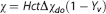
To calculate the blood susceptibility change caused by the stimulus, blood T₂ was measured in the sagittal sinus at baseline and stimulation (using a further oxygen block). The T₂ measurements were performed using an implementation of T₂-relaxation-under-spin-tagging. ²⁶ In our local implementation, spin tagging was performed using a pseudo-continuous inversion in the sagittal sinus superior to the imaging slice with a tag duration of 1.4 seconds and a postlabeling delay time of 150 milliseconds. A Malcom-Levitt T₂ preparation was used with a 10 milliseconds Carr-Purcell-Meiboom-Gill time, ²⁷ with effective TEs of 0, 40, 80, and 120 milliseconds, with four tag-control pairs acquired for each preparation time. As per Xu et al, ²⁸ global spoiling was used at the end of each TR, allowing a TR of 4 seconds and a total acquisition time of 2.2 minutes. Tag-control image pairs were motion corrected, subtracted, and the average value of a selected sagittal sinus voxel fit to obtain an estimate of T₂. The measured T₂ values were converted to venous oxygen saturation values according to Lu et al ²⁷ assuming a hematocrit of 0.4, and then into blood susceptibility values according to equation (3); ²⁹ where Δχ_do=4π·0.264.

$\chi =Hct{\mathrm{\Delta }}_{{\chi }_{do}}(1-Y_v)$

(3)

Analysis Methods

All data sets (simulations and volunteer studies) were analyzed using the two principal methods to calculate q, and therefore calculate the vessel size. In the first case, the average decay rates (ΔR₂∗ and ΔR₂) during signal plateau periods are used, in the second case a linear regression of ΔR₂∗ timepoints against ΔR₂ is used as per Jochimsen et al. ⁴ In each case, a refinement of the method is also investigated. For the plateau analysis, a t-test was used to identify statistically significant signal changes between baseline and stimulation periods as per Shen et al^{6, 7}. Only simulations that showed significant signal increases in both the GE and the SE data were included (P=0.0001). The regression analysis, which was originally evaluated with ordinary least squares (OLS), was extended via the use of a total least squares (TLS) regression. TLS allows for observational errors on both dependent and independent variables and so allows for uncertainties in both ΔR₂∗and ΔR₂. This is untrue for simple linear regression, which assumes the independent variable to be error free, and thus leads to attenuation bias when this is not the case. ³⁰

Calculated q values were converted into distributions of vessel radii using the Monte–Carlo modeled data and the relationships described in Figure 1. Unrealistic vessel sizes estimates, <1 μm and >70 μm, were discarded. Vessel distributions are summarized using the median, as is appropriate for non-normal distributions, however, in some instances mean values are also quoted for consistency with previous publications.

RESULTS

Simulations

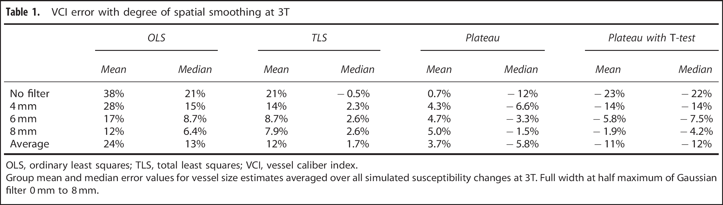
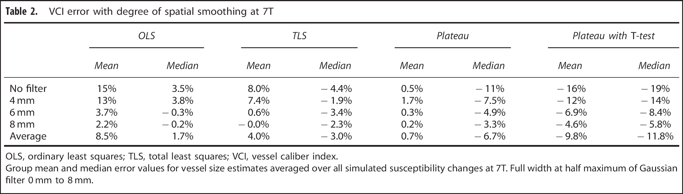
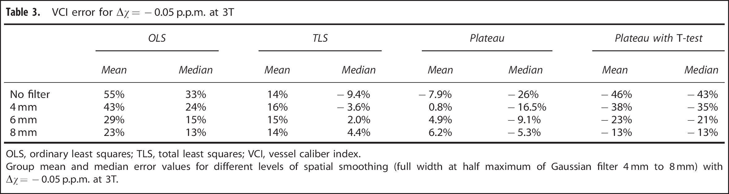
Using the estimated VCI distribution, the modeled data (without noise) predict a median q value of 4.0 (±0.4) at 3T and 5.6 (± 0.1) at 7T, corresponding to a median VCI of 11.8 μm (mean value 13.8 μm). Tables 1 and 2 summarize the mean and median errors in VCI values for the population analysis at 3T and 7T, respectively. The tables include summary results for all susceptibility changes and for each degree of spatial smoothing (separated by analysis method). Table 3 shows the errors for a modeled oxygen challenge (Δχ=−0.05 p.p.m.) at 3T, where the small susceptibility change emphasizes the bias present in each analysis method.

Table 1.

VCI error with degree of spatial smoothing at 3T

	OLS		TLS		Plateau		Plateau with T-test
	Mean	Median	Mean	Median	Mean	Median	Mean	Median
No filter	38%	21%	21%	−0.5%	0.7%	−12%	−23%	−22%
4 mm	28%	15%	14%	2.3%	4.3%	−6.6%	−14%	−14%
6 mm	17%	8.7%	8.7%	2.6%	4.7%	−3.3%	−5.8%	−7.5%
8 mm	12%	6.4%	7.9%	2.6%	5.0%	−1.5%	−1.9%	−4.2%
Average	24%	13%	12%	1.7%	3.7%	−5.8%	−11%	−12%

OLS, ordinary least squares; TLS, total least squares; VCI, vessel caliber index.

Group mean and median error values for vessel size estimates averaged over all simulated susceptibility changes at 3T. Full width at half maximum of Gaussian filter 0 mm to 8 mm.

Table 2.

VCI error with degree of spatial smoothing at 7T

	OLS		TLS		Plateau		Plateau with T-test
	Mean	Median	Mean	Median	Mean	Median	Mean	Median
No filter	15%	3.5%	8.0%	−4.4%	0.5%	−11%	−16%	−19%
4 mm	13%	3.8%	7.4%	−1.9%	1.7%	−7.5%	−12%	−14%
6 mm	3.7%	−0.3%	0.6%	−3.4%	0.3%	−4.9%	−6.9%	−8.4%
8 mm	2.2%	−0.2%	−0.0%	−2.3%	0.2%	−3.3%	−4.6%	−5.8%
Average	8.5%	1.7%	4.0%	−3.0%	0.7%	−6.7%	−9.8%	−11.8%

OLS, ordinary least squares; TLS, total least squares; VCI, vessel caliber index.

Group mean and median error values for vessel size estimates averaged over all simulated susceptibility changes at 7T. Full width at half maximum of Gaussian filter 0 mm to 8 mm.

Table 3.

VCI error for Δχ=−0.05 p.p.m. at 3T

	OLS		TLS		Plateau		Plateau with T-test
	Mean	Median	Mean	Median	Mean	Median	Mean	Median
No filter	55%	33%	14%	−9.4%	−7.9%	−26%	−46%	−43%
4 mm	43%	24%	16%	−3.6%	0.8%	−16.5%	−38%	−35%
6 mm	29%	15%	15%	2.0%	4.9%	−9.1%	−23%	−21%
8 mm	23%	13%	14%	4.4%	6.2%	−5.3%	−13%	−13%

OLS, ordinary least squares; TLS, total least squares; VCI, vessel caliber index.

Group mean and median error values for different levels of spatial smoothing (full width at half maximum of Gaussian filter 4 mm to 8 mm) with Δχ=−0.05 p.p.m. at 3T.

The simple regression technique (OLS) produces a large overestimation of VCI at 3T, reducing with increased smoothing or susceptibility change. The TLS regression significantly reduces this overestimation taking the group median error down from 13% to 1.7%. However, the plateau analysis results in a consistent underestimation of the median value, with a group error of −5.8%. The inclusion of a t-test increases this error to −12%. The majority of the error in the t-test approach is because of underestimations of q in low CNR situations, with a maximum error of −43% (for no smoothing and Δχ=−0.05 p.p.m.). Increasing levels of smoothing reduce this error to around the 13% level for a smoothing kernel of 8 mm FWHM.

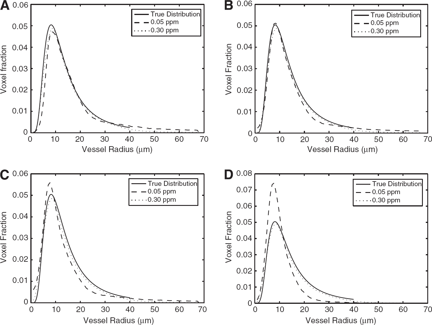
Figures 2A–2D show estimated VCI distributions for Δχ=−0.05 and −0.3 p.p.m. (spatial smoothing=6 mm FWHM) for each analysis method. It is clear from the figures that the plateau analysis shifts the modal value to the left, increasing the number of small vessel estimates. The OLS analysis shifts the modal value to the right. Introducing a t-test preferentially removes large vessel estimates, with increasing bias for smaller susceptibility changes. The TLS analysis shows reduced bias compared with the OLS analysis, more closely matching the true distribution. Increasing Δχ reduces the bias present in all analysis techniques.

Figure 2.

Modeled probability density estimates of vessel radii for each analysis method at 3T with an assumed vessel distribution (true distribution). Modeled data derived from 6 mm full width at half maximum smoothed data sets and susceptibility changes −0.05 and −0.3 p.p.m. Ordinary least squares analysis (A), total least squares (B), plateau analysis (C), and plateau analysis with t-test (D).

As shown in Table 2 the OLS estimates of VCI at 7T show only a modest overestimation in the median (group value of 3.5%), even with no spatial smoothing. Overall, the errors at 7T are much reduced compared with 3T. However, there is still a surprisingly high bias introduced by the t-test method (for small Δχ), which is apparent in the summary statistics. The cause of this anomaly is likely because of the sharper decrease in SE signal with vessel size, the same reason for increased q values at 7T. Thus, the statistical test is more heavily biased to larger vessel sizes at higher field strengths.

In Vivo Validation

Measurements of the change in intravascular T₂ (as a result of the hyperoxic stimulus) were made with a T₂-relaxation-under-spin-tagging sequence. The average T₂ value at baseline was found to be 65 milliseconds, increasing to 75 milliseconds during hyperoxia, which is equivalent to an intravascular susceptibility change of −0.057 p.p.m. The closest modeled susceptibility change of −0.05 p.p.m. was used to calculate radius estimate from the volunteer data.

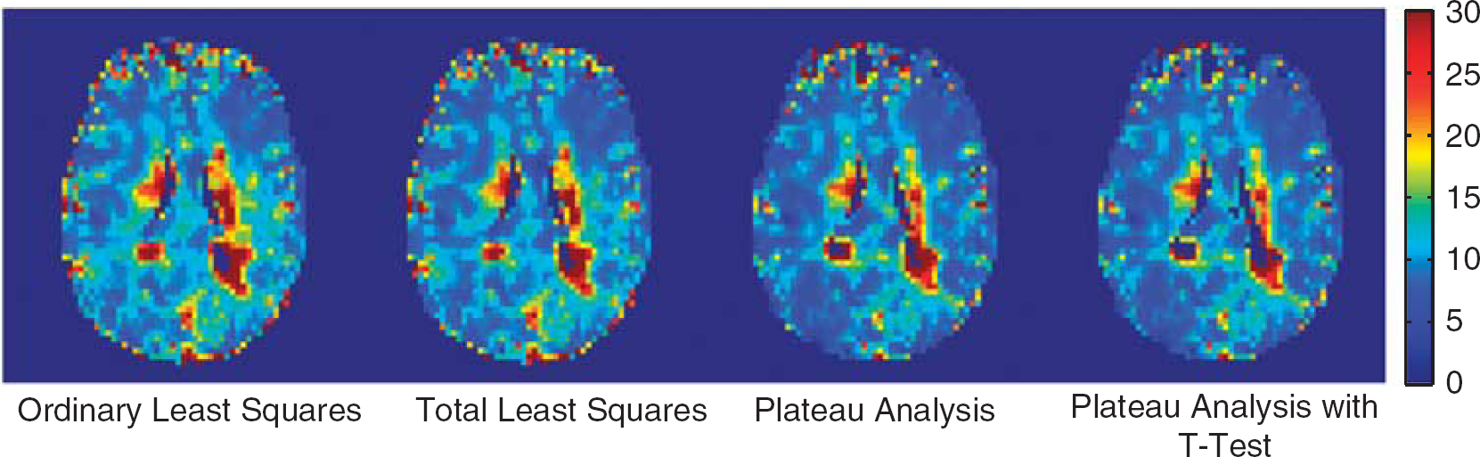
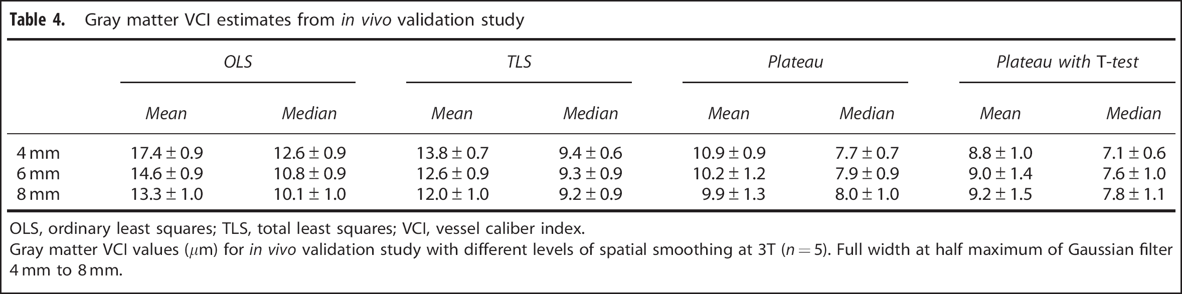
Figure 3 shows example parameter maps for each of the analysis methods (OLS, TLS, plateau and plateau plus t-test) from the acquired volunteer data. The maps appear generally similar, with an apparent reduction in vessel size with the plateau techniques. The variation in vessel size with analysis method and smoothing level is summarized in Table 4. As with the modeled data, OLS estimates are consistently greater than TLS, while the median TLS value is relatively insensitive to the degree of spatial smoothing. Plateau estimates of VCI are less than with the regression techniques, and are further reduced by including a t-test. This is consistent with the modeled data presented in Table 3, which predicts errors of 13%, 4.4%, −5.3%, and −13% for a susceptibility change of −0.05 p.p.m. and an 8 mm spatial smoothing kernel. Given the correspondence between the results and the expected errors, we can infer that the true mean and median VCI values in this subject group are approximately 11 and 8.5 μm, respectively. These values are obtained by choosing VCI values that best correspond to the modeled error in each of the analysis methods.

Figure 3.

Example mean vessel caliber estimates (μm) from an individual subject. The same slice is shown analyzed with each of the investigated methodologies.

Table 4.

Gray matter VCI estimates from in vivo validation study

	OLS		TLS		Plateau		Plateau withT-test
	Mean	Median	Mean	Median	Mean	Median	Mean	Median
4 mm	17.4±0.9	12.6±0.9	13.8±0.7	9.4±0.6	10.9±0.9	7.7±0.7	8.8±1.0	7.1±0.6
6 mm	14.6±0.9	10.8±0.9	12.6±0.9	9.3±0.9	10.2±1.2	7.9±0.9	9.0±1.4	7.6±1.0
8 mm	13.3±1.0	10.1±1.0	12.0±1.0	9.2±0.9	9.9±1.3	8.0±1.0	9.2±1.5	7.8±1.1

OLS, ordinary least squares; TLS, total least squares; VCI, vessel caliber index.

Gray matter VCI values (μm) for in vivo validation study with different levels of spatial smoothing at 3T (n=5). Full width at half maximum of Gaussian filter 4 mm to 8 mm.

DISCUSSION

Blood oxygenation level-dependent-mediated VSI offers a novel method for quantifying vessel sizes and vessel size changes in vivo. However, because of the relatively low CNR of the method, care must be taken when analyzing and comparing results. Here we have explored the noise sensitivity of different analysis methods using a simulated BOLD acquisition. The results show significant CNR-dependent variations in calculated q values, and therefore vessel size estimates.

The use of a linear regression to assess the ratio q provides a model-free analysis method, which should be unaffected by regional changes in hemodynamic latency and/or delay. ⁴ Although this may prove important in certain disease states, it is also insensitive to any delayed hypercapnic response between healthy gray and white matter. However, standard regression techniques have long been known to underestimate the gradient because of noise in the independent variable. ³¹ As the regression is used to estimate 1/(ΔR₂∗/ΔR₂), this can lead to an overestimation of q and hence vessel size. Here we include a TLS regression to mitigate this effect. The modeling results show that the TLS regression removes much of the overestimation in vessel size, correcting a median overestimation of 13% to only 1.7% at 3T.

As large vessels produce a small ΔR₂, any reduction in this because of noise can lead to a significant overestimation of q. One method to remove these uncertain estimates, proposed by Shen et al, ⁶ is to use a t-test to accept estimates only if there is a significant increase in GE and SE signals between rest and stimulation. However, above approximately 10 μm the change in GE signal should always be significantly greater than the change in SE. Therefore, for the most part, this is really a test for significant changes in the SE signal. As ΔSE decreases with vessel size, great care must be taken not to exclude legitimate voxels that are dominated by large vessels. In addition, any estimates where noise adds to ΔSE such that it passes the t-test will be accepted, while estimates where noise reduces ΔSE below significance will be rejected. Our simulations show that this biased rejection causes an increased underestimation of the mean and median vessel size. A mean reduction in vessel size of approximately 30% to 40% is predicted in low CNR situations (small Δχ and minimal spatial smoothing), this corresponds well with the 40% change observed by Shen et al. ⁶

It could be argued that the distribution used in our modeling is unrepresentative of the true vessel distribution, including an unrealistic number of large vessels. In our model distribution, 20% of vessels have a radius >20 μm, while in recent in vivo studies Perez-Barcena et al ³² suggest that only 10% of vessels fall in to this range. However, this difference could be explained by BOLD sensitivity to large veins that were excluded from the study. In addition, our validation study revealed a consistently lower estimate of vessel size with the t-test approach that reduced with the level of spatial smoothing (as predicted by the modeling). Although the motivation for the t-test approach is to remove unrealistic estimates of large vessels, it appears that the level of significance chosen is such that it includes a significant proportion of large vessel estimates in low CNR situations. This phenomenon becomes increasingly important when comparing acquisitions performed with different apparatus and gas challenges. For instance, if this approach is used to compare the vessel size response to hyperoxia and hypercapnia (where an SNR increase is expected because of an increase in Δχ), then care must be taken to analyze the same vessel populations to avoid biasing the results.

If the estimated mean vessel size in this study (11 μm) is compared with the reported VCI estimates in Shen et al, ⁶ we can see that a reduction of approximately 40% is required to match the estimated vessel size of 6.5 μm. As previously observed, this reduction is similar to the impact of the t-test in their study, and implies a low CNR compared with our modeling results. The low CNR is plausible as the results in this study are derived from a 32-channel head coil rather than the 8-channel coil used by Shen et al. Comparing our result to Jochimsen et al ⁴ , it requires a 22% increase in the mean vessel estimate to match their estimate of 13.4 μm; while our modeling can only account for 10% of this increase, the remainder can be explained by the vasodilatory effect of CO₂ (ref. 22). Assuming any increase in blood volume is the result of an increase in the radius, the required 10% increase corresponds to a 20% blood volume increase, well within the range measured by Lee et al. ²³

The sensitivity to CNR in this study has been examined through the use of different degrees of spatial smoothing. The approach offers the opportunity to investigate the noise dependence of the analysis methods without the need to acquire multiple data sets. In addition, it is relevant to practical BOLD-VSI implementations, which will typically use some degree of Gaussian smoothing. However, there is the possibility that distribution of vessel sizes under examination will vary with the degree of spatial smoothing. For example, a large degree of spatial smoothing could enhance the contribution of surface draining veins to nearby tissue, thus increasing the median VCI. This phenomenon is more likely to present itself in the in vivo experiments, as the simulations implicitly assume a uniform distribution. However, given the qualitative agreement between the simulations and in vivo data, this effect appears to be small in comparison with the investigated CNR dependence.

Our results highlight the important interaction between CNR and BOLD-VSI analysis methodology. The low CNR inherent in BOLD-VSI studies, particularly at lower field strengths, can lead to both large overestimation (OLS) and underestimation (t-test) of the mean vessel size. We have shown how the use of a more appropriate regression method (TLS) removes much of this bias. Although the underestimation observed with the t-test methodology goes some way toward explaining the differences observed in vessel size estimates made by Jochimsen et al^{4, 13} and Shen et al.^{6, 7} Further differences between the results are expected because of vasodilatory effect of CO₂( ²² ) and are within the physiologic range of blood volume changes.

To increase the reliability and robustness of BOLD-VSI, it is important to consider the influence of the CNR on the analysis method. Ideally, data should be acquired and smoothed to achieve a CNR such that the analysis method minimally influences the results. If this is not possible then the effect of all processing steps should be understood and characterized to avoid significant bias. At 7T, our modeling shows that all analysis methods result in a group error of 10% or less for large (−0.3 p.p.m.) susceptibility changes. At lower field strengths and with smaller susceptibility changes, the choice of analysis method becomes increasingly critical and great care is required.