
Abstract
Blood–brain barrier damage, which can be quantified by measuring vascular permeability, is a potential predictor for hemorrhagic transformation in acute ischemic stroke. Permeability is commonly estimated by applying Patlak analysis to computed tomography (CT) perfusion data, but this method lacks precision. Applying more elaborate kinetic models by means of nonlinear regression (NLR) may improve precision, but is more time consuming and therefore less appropriate in an acute stroke setting. We propose a simplified NLR method that may be faster and still precise enough for clinical use. The aim of this study is to evaluate the reliability of in total 12 variations of Patlak analysis and NLR methods, including the simplified NLR method. Confidence intervals for the permeability estimates were evaluated using simulated CT attenuation-time curves with realistic noise, and clinical data from 20 patients. Although fixating the blood volume improved Patlak analysis, the NLR methods yielded significantly more reliable estimates, but took up to 12 x longer to calculate. The simplified NLR method was ~4 x faster than other NLR methods, while maintaining the same confidence intervals (CIs). In conclusion, the simplified NLR method is a new, reliable way to estimate permeability in stroke, fast enough for clinical application in an acute stroke setting.
INTRODUCTION
Computed tomography (CT) perfusion (CTP) imaging, or dynamic contrast enhanced CT, is frequently used for the evaluation of acute stroke.
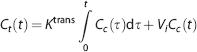
It has previously been hypothesized that blood–brain barrier damage is a predictor for hemorrhagic transformation in acute stroke.1-3 With CTP imaging, blood–brain barrier damage can be quantified by measuring vascular permeability. Along with other perfusion parameters, including cerebral blood volume (CBV) and flow (CBF), vascular permeability is a tissue property that can be estimated by comparing tissue attenuation-time curves with the curve of a reference artery or arterial input function (AIF). While CBF and CBV can be measured by imaging the first-pass bolus passage, leakage of contrast agent to the extravascular space is a slower process, only discernible in a delayed phase, and therefore requiring longer scan times. In stroke imaging, permeability is most frequently estimated using linearized regression, that is, by graphical analysis of a Patlak plot.1,3-6 This technique transforms the data in the attenuation–time curves so that, in case of irreversible leakage, the data points lie on a straight line when the capillary tracer concentration reaches steady state. The permeability transfer constant
The Patlak method is preferred in the acute stroke setting, because it is fast, despite some inherent drawbacks. First, due to the linearized regression, only the steady-state data points, that is, the last part of the scan, can be used. The estimated values are therefore dependent on the definition of the onset of this steady state, and potentially useful information in the first part of the signal is disregarded. Second, linear least-squares regression assumes that the errors on the samples are normally distributed. For linearized data, this is not the case and therefore the result will not be an optimal least-squares fit. 7 Third, other parameters, such as the CBV and CBF, are estimated using a different method, which usually includes Gaussian or gamma variate curve fits, or a regularized inverse filter. 8 Because two different methods are used for estimating parameters that essentially describe the same tissue model, the results may disagree. For example, the CBV, which should measure the intravascular volume only, may be overestimated by methods that do not take into account the additional extravascular distribution volume due to increased permeability of the blood–brain barrier.9,10
As an alternative to the Patlak method, the use of a tissue perfusion model applied with nonlinear regression (NLR) uses the full length of the attenuation-time curves, does not transform the measurement errors, and allows for a simultaneous measurement of all perfusion parameters. For these reasons, NLR methods may provide a superior alternative to the use of Patlak plots in stroke imaging.2,11,12 However, NLR methods rely on iterative algorithms that are relatively time consuming. A rapid diagnosis is crucial for treatment of acute stroke; and therefore, these methods may not be practical in an acute stroke setting.
The purpose of this study was to compare the reliability and computation time of permeability estimation using various implementations of the Patlak method and NLR methods using clinical and simulated data. In addition, a novel simplified NLR method is proposed as a faster potential alternative to existing NLR methods.
MATERIALS AND METHODS
This section first describes a first-pass bolus model that is required for the calculation of some of the Patlak methods. Second, details are provided for the theory and technical implementation of different Patlak and NLR methods. Third, a novel method for NLR, based on the adiabatic approximation to the tissue homogeneity (TH) (AATH) model,
13
is introduced. Table 1 summarizes all in this study included methods for estimating permeability. Finally, methods for evaluating the models' reliability of estimating
An overview of the studied methods and their free and fixed parameters, according to Equation 5
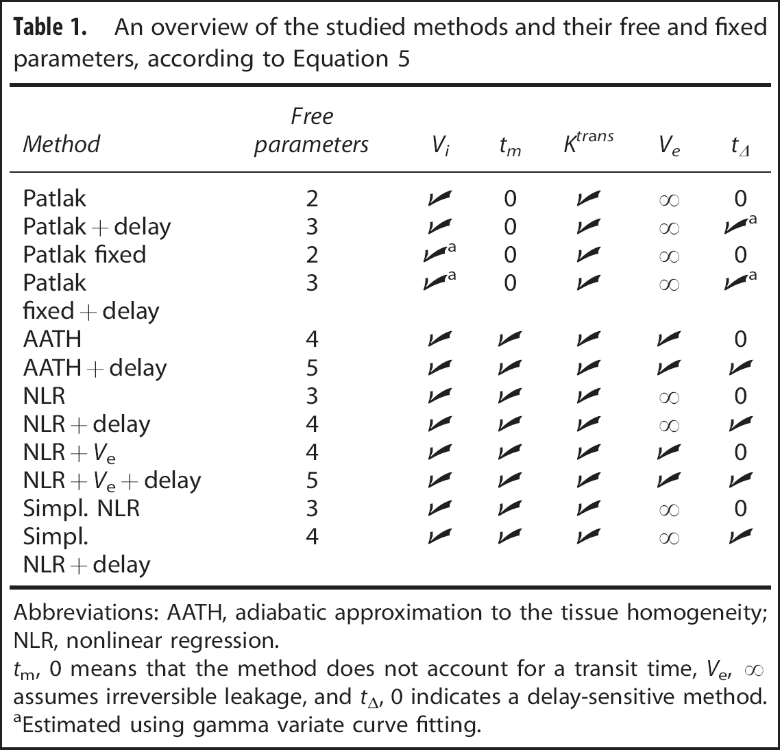
Abbreviations: AATH, adiabatic approximation to the tissue homogeneity; NLR, nonlinear regression.
aEstimated using gamma variate curve fitting.
First-Pass Bolus Fitting
Some implementations of the Patlak plot (described below) require estimates of the CBV and time-to-peak (TTP). To obtain these values, and estimates for the CBF and mean transit time (MTT), the attenuation–time curves can be analyzed using a broad range of methods. Despite that more sophisticated methods exist for estimating the CBF and MTT, this study uses gamma variate curve fitting of the first-pass bolus for obtaining the CBV and TTP, because the variability in outcome between the methods for estimating these parameters was found to be very small. 8
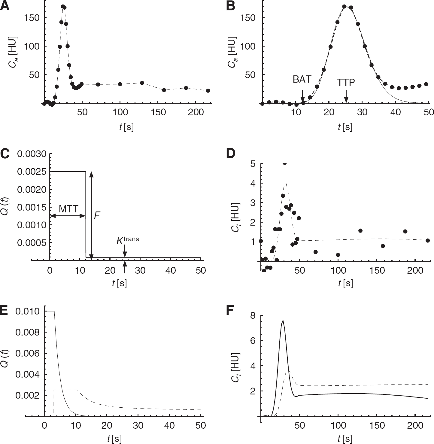
A gamma variate fit gives a robust estimate of the area under the curve (AUC) and TTP of the first-pass bolus in the attenuation–time curve.14-16 Subsequently, the CBV can be estimated by dividing the AUC of the tissue curve by the AUC of the AIF. 10 The bolus arrival time (BAT), which is in this study used to define the start of contrast enhancement, is defined as the 0. 05% quantile of the gamma variate fit (Figure 1B).
An overview of the arterial input function (AIF), and simulated impulse response functions (IRFs) and tissue attenuation–time curves. (
Patlak Linearized Regression
An underlying assumption of Patlak analysis is that the vascular leakage is irreversible during the acquisition time. In that case, the total tracer concentration in the tissue,
If both sides of the equation are divided by
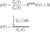
Equation 1 shows that when a linear fit
The onset of the delayed phase, in which steady state is reached, is in this study empirically defined as the arterial TTP plus 3.5 x the standard deviation of the first-pass bolus, measured using a gamma variate curve fit as described above. This is a reliable method, because gamma variate fits give a robust estimate of the width and position of the first-pass bolus peak.
Patlak Analysis with a Fixed Offset
The blood volume can be read from the Patlak plot (Equation 1). Alternatively, if an estimate of
For comparison, both the ‘standard’ and the ‘fixed’ Patlak methods are examined (Table 1).
Patlak Analysis with Delay Correction
In CTP imaging, the arterial concentration
In line with this, both the ‘standard’ and ‘fixed’ Patlak methods are also extended with a delay correction (Table 1). The gamma variate fits to the AIF and tissue curves provide a robust estimate of the TTP values if the leakage is small.
Nonlinear Regression
A Perfusion Model for Nonlinear Regression
Tissue perfusion is frequently modeled as a linear time-invariant system. Under that assumption the dynamics of the tracer concentration in the tissue can be described as the convolution of the AIF with a characteristic impulse response function (IRF). An IRF can be thought of the attenuation–time curve of a small tissue volume in response to an infinitesimal short AIF.
The NLR technique in this study uses a mathematical tissue response model to describe the IRF. The convolution of the measured AIF with a computed IRF gives an estimate of the true attenuation–time curve of the tissue volume. Non-linear regression is used to iteratively adapt any of the parameters in the mathematical model, such as the blood volume and transit time, to minimize the error between this estimate and the measured attenuation–time curve.
Sawada

In Equation 2,
The AATH model describes the tracer concentration dynamics in a small volume containing a single capillary vessel with a uniform (plug) flow. In reality, however, brain tissue is heterogeneous and even a small volume contains capillaries with variable lengths. This heterogeneity causes a small tissue volume to have a distribution of transit times
In this equation, QAATH(
Bredno

Solving the model assumes knowledge about the capillary concentration. In practice, due to resolution and noise limits, the AIF is measured in a large artery, often located away from the tissue of interest, so extra travel time for the contrast to arrive in the tissue needs to be accounted for. This is particularly important in the study of tissue regions that are fed through collateral routes. It has been shown that the performance of other deconvolution methods is improved by making them delay insensitive.23,24 This can be performed by introducing an additional parameter for the delay,

The parameter
The AATH model (Equation 2), and also the tracer kinetic models used by Larson
Simplified Nonlinear Regression
Nonlinear regression with five unknown variables is a computational intensive task. Bottlenecks involve the calculation of exponentials, divisions, and a convolution operation in each iteration.
However, the computational complexity is highly reduced by two simplifications to

What is even more important, is that it is now no longer necessary to apply a convolution in each iteration. The convolution of
The integral of
This simplified version of
Model Variations
A total of 12 different methods were compared. Both Patlak and the NLR methods include parameters that are either free for estimation or fixed to a predefined value. The full tissue response model
If global optima are found, which is not guaranteed, then increasing the number of free parameters will result in a better fit (a higher
All methods were implemented in a similar manner in C routines that are accessible in Matlab (version 2011b, The MathWorks Inc., Natick, MA, USA) through the Matlab MEX programming interface.
Simulations were applied to gain insight in the response of the models to noise and varying perfusion parameters, and CT brain perfusion scans were analyzed to estimate the reliability of the measured permeability in clinical practice.
Simulated Data
To evaluate in a setting with controlled noise levels and perfusion parameters, tissue attenuation–time curves were simulated by convolving a measured AIF with a generated IRF, and adding Gaussian noise. An AIF (Figure 1A) was extracted from a clinical CTP brain scan as described below.
The AATH model20,13 (Equation 2) was used to generate the IRFs, because the TH model is thought to match the physiology of the brain better than other published models.19,12 The blood flow
The noise level,
In the remaining three sets, one out of three parameters was varied while the others were fixed to 1 HU for the noise level, 0.5 mL/min per 100 g for the
The simulated attenuation curves were analyzed using all methods listed in Table 1, while keeping track of the mean, standard error, and average approximate standard error of the estimated
Figures 1A, 1C, and 1D give an overview of the measured AIF, and the default IRF, and attenuation–time curve. Both the IRF and the AIF were band limited using a Bartlett kernel (triangular) with a full width at half maximum of 4 seconds. Figures 1E and 1F show how the shape of
Computed Tomography Brain Perfusion Scans
Data Acquisition
The CTP scans of 20 acute ischemic stroke patients that participated in the Dutch Acute Stroke Trial (NCT00880113) were included (chronological order). Dutch Acute Stroke Trial is large prospective multicenter observational cohort study, approved by the institutional medical ethics committee (METC), and in accordance with the Good Clinical Practice guidelines as provided by the International Conference on Harmonisation (ICH-GCP) and Dutch act on medical research involving human subjects (WMO).
For CTP, 40 mL of nonionic contrast agent (Iopromide, Ultravist, 300 mg/mL iodine; Bayer HealthCare Pharmaceuticals, Berlin, Germany) was injected intravenously at a rate of 6 mL/s followed by a 40-mL saline flush at a rate of 6 mL/s. The scans were acquired using a Philips Brilliance iCT scanner (Philips Healthcare) at 80 kVp and 150 mAs/rot and a field-of-view of ~200 × 200 mm2 with an axial coverage of 65 mm at most. The total acquisition time was 210 seconds, divided into 25 frames with a 2-second interval, followed by 6 frames with a 30-second interval (Figure 1A). The scans were reconstructed in a 512 × 512 matrix with filtered back-projection and a Philips UB filter.
Preprocessing
The open source registration toolbox Elastix 29 was used to register the original, 3D high-resolution CTP data (voxel size 0. 39 × 0.39 × 0.83 mm3) to the first time frame. Next, slabs of six adjacent registered slices were averaged to obtain 8 to 13 slabs of 5 mm per volume.
Noise reduction is crucial in CTP analysis. Because of the limited radiation dose, the unfiltered scans have a very low signal-to-noise ratio, especially in the areas with low perfusion where blood–brain barrier damage is to be expected. Sophisticated noise filtering, where e.g. temporal information is used to adapt the filter kernel to its spatial neighborhood, is therefore desirable.
A temporal Gaussian filter with a standard deviation of 4 seconds, followed by a 3D bilateral filter (the time-intensity profile similarity filter, or TIPS) 30 with a spatial standard deviation (σd) of 4 mm and a profile-similarity standard deviation (σζ) of 50 HU2 were applied to reduce the noise with a minimum loss of resolution.
Arterial Input Function
The AIF was semiautomatically selected either in an internal carotid or in the basilar artery by drawing a circular region of interest in which the attenuation curve with the highest enhancement was chosen. To correct the AUC of the AIF for partial volume effect, a venous output function was in the same way semiautomatically selected in a great sinus perpendicular to the slices, 31 which is in line with the clinical scan protocol. A gamma variate curve was fitted to both the AIF and venous output function to estimate their AUCs, the arterial BAT, and the steady-state concentration time (see First-Pass Bolus Fitting section).
Postprocessing
Only the voxels that were classified as penumbra (tissue at risk) were used for statistical analysis. This was performed because the signal-to-noise ratio of the attenuation–time curves in the infarct (irreversible ischemia) is low, which might hamper reliable measurements. The
To extract the penumbra and exclude vessels, tissue types in the brain were segmented based on the CT values in the first frames of the filtered scan, before the BAT. By removing voxels with a CT value of <17 HU or >55 HU (unenhanced), air, fat, and bone are excluded from the analysis, while gray and white matter remain. Within the brain tissue, the infarct and penumbra were defined based on the CBV and relative MTT that were estimated by the simplified NLR method.
To calculate the relative MTT, a symmetry plane was manually drawn to separate the hemispheres. The original MTT map is mirrored over this plane and blurred by a 3D Gaussian kernel with a standard deviation of 3 mm. The relative MTT values are found by dividing the original MTT map by the mirrored, blurred map.
Wintermark
A correction factor
Statistical Analysis
Besides the
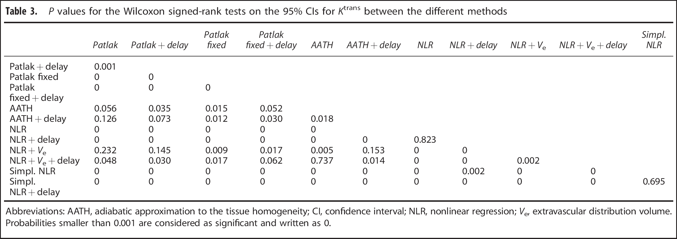
The estimated values and CIs in the penumbra regions were averaged per patient and a Wilcoxon signed-rank test was applied to each pair of methods to test if the differences between the methods were significant (
RESULTS
Simulated Data
Figure 2A shows the standard error on the
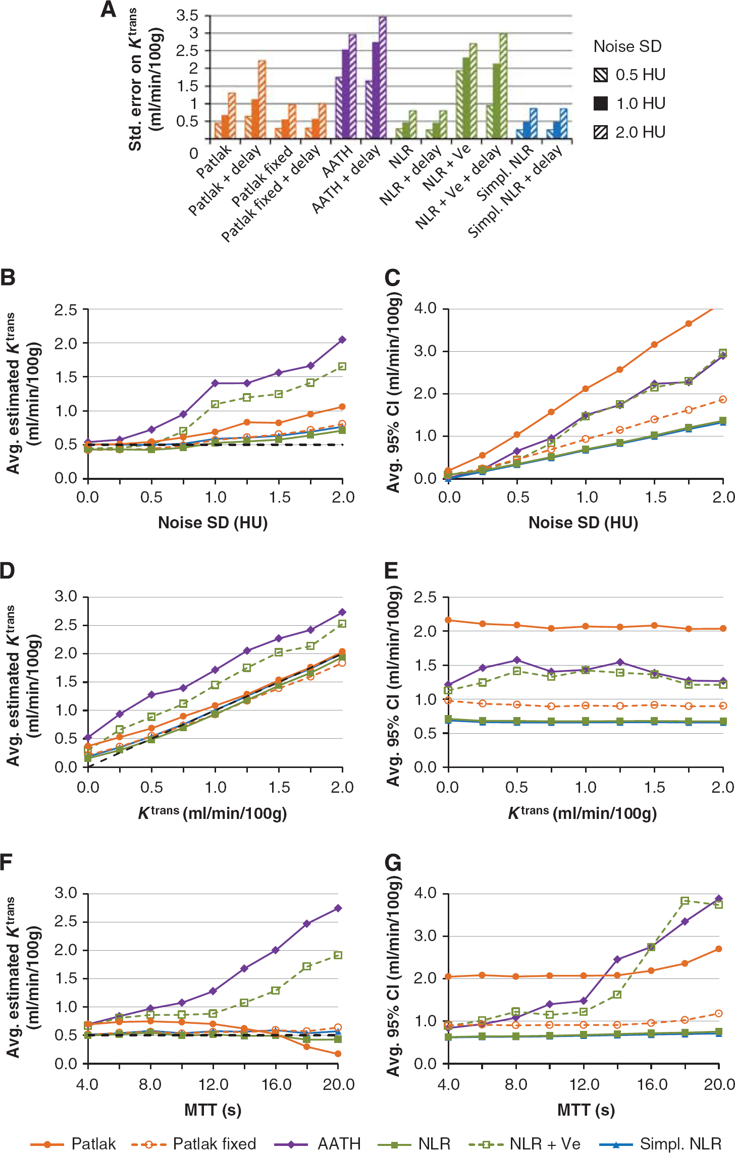
Graph (
Because the steady-state time was defined as the TTP plus 3.5
The results showed that noise gives a positive bias to the average
In all cases with noise, the NLR methods with irreversible leakage were found to have the smallest CIs, while the standard Patlak method had the largest CI, implying that it is least reliable (Figures 2C, 2E, and 2G). All methods gave estimates of which the width of the CI scaled linearly with the noise level (Figure 2C). Figure 2E shows that the confidence of the estimation did not scale with the
Computed Tomography Brain Perfusion Scans
The
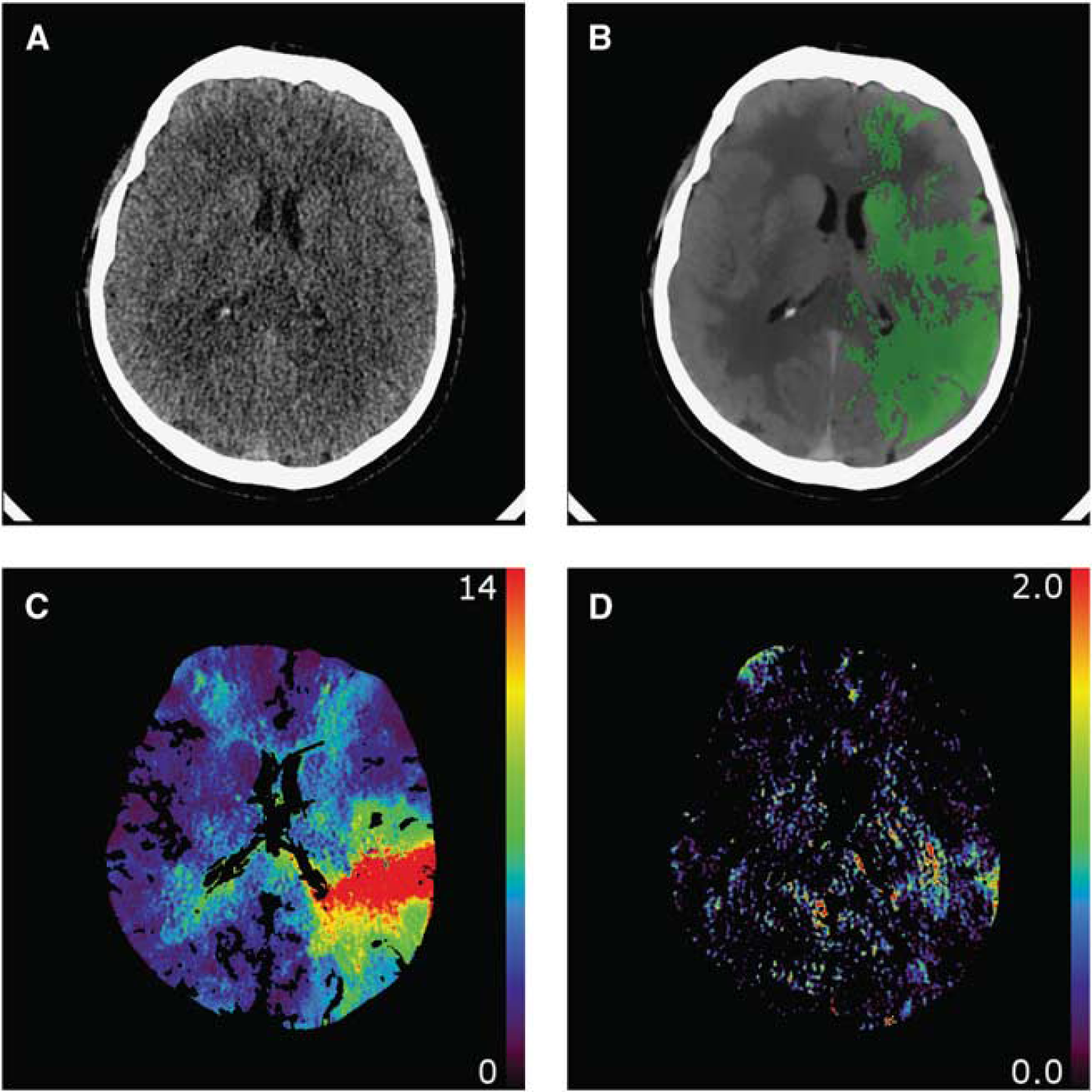
An example of (
There was a large variance in
The
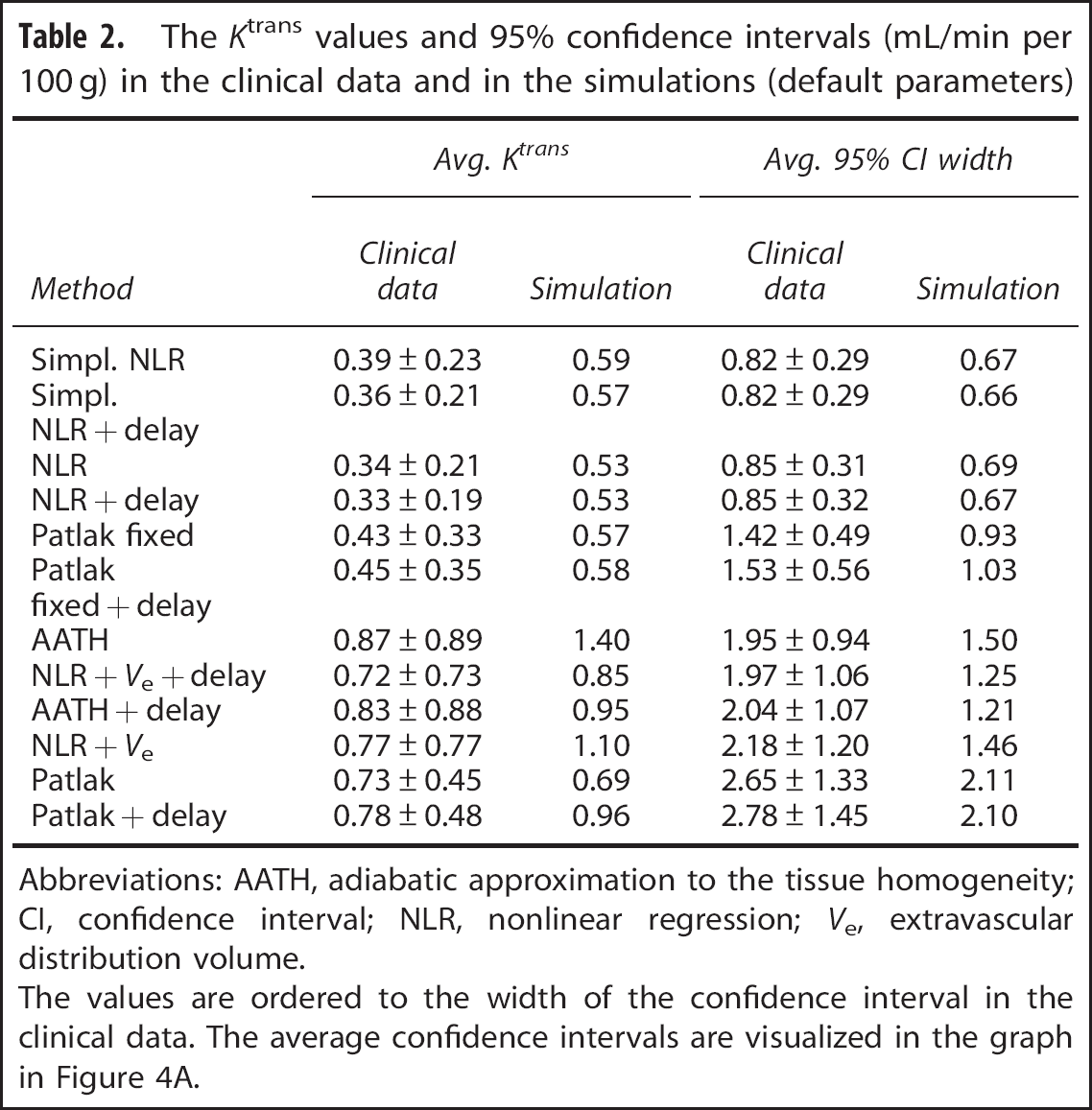
Abbreviations: AATH, adiabatic approximation to the tissue homogeneity; CI, confidence interval; NLR, nonlinear regression;
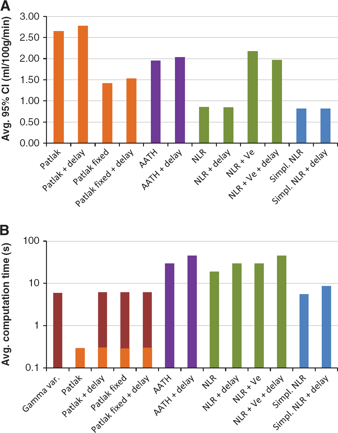
The values are ordered to the width of the confidence interval in the clinical data. The average confidence intervals are visualized in the graph in Figure 4A.
Abbreviations: AATH, adiabatic approximation to the tissue homogeneity; CI, confidence interval; NLR, nonlinear regression;
Because the steady-state time for Patlak analysis was defined as the TTP plus 3.5
Figure 4A, and Table 2 together with Table 3 show that the
(
Figure 4A also shows that fixating the CBV significantly improved the reliability of the Patlak estimates.
The delay correction had a minor effect on the CIs. With
Also, the MTT distribution parameter
Figure 4B gives an overview of the average computation time for each method. It is not surprising that the simplest method, standard Patlak, was the fastest with 0.3 second per slice (512 × 512 pixels and 31 time frames). The other Patlak methods require additional input provided by a gamma variate fit, extending the computation time to 5.9 seconds per slice. The simplified NLR methods had computation times of respectively 5 and 9 seconds per slice, where the other NLR methods required between 19 and 45 seconds.
DISCUSSION
This study uses CIs to compare the reliability between different methods for estimating
‘Reliability’ is a nonscientific term that should be used with care. Some ‘reliability metrics’, like the Akaike information criterion,
34
quantify the goodness of fit of a model. For two reasons, however, this type of metric is not applicable to this study. First, the Patlak fits are applied to different (linearized) data than the nonlinear fits; and therefore, the goodness of fit between these methods may not be compared. Second, the reliability of a single parameter,
A wider CI means a larger standard deviation in repeated measurements. For
The standard Patlak method was found to be two to three times less reliable than the NLR and simplified NLR method in both the simulated and clinical cases. However, fixating the CBV to a value estimated with a more sophisticated method, which is usually available anyway, roughly doubles its reliability. This means that fixating the CBV in the Patlak plot is a simple but very effective way to enhance the reliability of the permeability estimates in general.
The standard Patlak method showed a decrease in reliability for long transit times. The performance of this method could in those cases probably be increased by determining the steady state of the tissue attenuation curve instead of the AIF, as was performed in this study. A longer MTT means that it takes more time for the capillary concentration to reach a steady state and therefore fewer samples should be included in the Patlak plot.
The addition of a delay time
The shape of the MTT distribution, controlled by the parameter
The simulations showed that the AATH and NLR +
On many points, the NLR method provides a more sound theoretical basis than Patlak analysis for permeability analysis, and gamma variate fits or deconvolution8,35 for perfusion analysis. First, the NLR method does not make any assumptions of the shape of the attenuation curves themselves, but rather on the process that transforms the AIF into a tissue curve. The curves do not necessarily need to have a gamma variate-like profile, nor do they have to reach a steady state. A potential second pass bolus due to recirculation does not hamper the analysis. Second, at about
A disadvantage of NLR is that it is an iterative method, and so a straightforward implementation is time consuming. This is most likely the reason why currently this technique is not much used in CTP analysis yet. The simplified NLR method, however, tackles two bottlenecks by omitting the need for convolutions and the calculation of exponentials, and is thereby at least four times faster than the full NLR methods. By further increasing the performance using, e.g., parallel computing or GPU acceleration the analysis of high-resolution volumes in a clinical setting might be feasible.
In conclusion, the CI, and thereby the reliability, of the simplified NLR method is similar to the full NLR methods, and better than the Patlak methods in both the simulations and clinical measurements. The simplified NLR analysis just takes 5 seconds per 512 × 512 slice, making it suitable for time-critical clinical use. The simplified NLR method therefore seems to be a superior alternative to Patlak analysis. Further research is required to evaluate the predictive value of the simplified NLR method for hemorrhagic transformation in acute ischemic stroke.
The techniques described in this study are potentially applicable to other purposes as well, like tumor assessment using dynamic contrast enhanced magnetic resonance imaging or positron emission tomography, even though the signal-to-noise ratio and kinetics might differ.
DISCLOSURE/CONFLICT OF INTEREST
The authors declare no conflict of interest.