Robust Fitting of [ 11 C]-WAY-100635 PET Data

Abstract

Fitting of a positron emission tomography (PET) time–activity curve is typically accomplished according to the least squares (LS) criterion, which is optimal for data having Gaussian distributed errors, but not robust in the presence of outliers. Conversely, quantile regression (QR) provides robust estimates not heavily influenced by outliers, sacrificing a little efficiency relative to LS when no outliers are present. Given these considerations, we hypothesized that QR would improve parameter estimate accuracy as measured by reduced intersubject variance in distribution volume (V _T ) compared with LS in PET modeling. We compare V _T values after applying QR with those using LS on 49 controls studied with [¹¹C]-WAY-100635. QR decreases the standard deviation of the V _T estimates (relative improvement range: 0.08% to 3.24%), while keeping the within-group average V _T values almost unchanged. QR variance reduction results in fewer subjects required to maintain the same statistical power in group analysis without additional hardware and/or image registration to correct head motion.

Introduction

In the analysis of positron emission tomography (PET) time activity curves (TACs) data, model fitting is typically accomplished by using nonlinear regression algorithms (Zubieta et al, 1998). The preponderance of estimation in regression modeling has been carried out according to the least squares (LS) criterion, which is known to be optimal and to coincide with the maximum likelihood estimator for data having Gaussian distributed errors, but not robust in the presence of outliers or other influential points, or for other error distributions. In such a case, the LS criterion may still be used and may still deliver reasonable estimates, but other criteria may provide better estimates. For instance, when the errors follow a double-exponential distribution (i.e., Laplace), the maximum likelihood estimator of the regression parameters requires minimizing the sum of the absolute values, instead of the squares, of the differences between the experimental data and the prediction of the considered model. Both these estimation techniques are special cases of the so-called Lp-norm estimators. The choice of p—the scalar representing the power to which each sampling time difference between model prediction and experimental data is raised to in the weighting sum that has to be minimized (Gonin and Money, 1989)—that will allow for efficient and robust estimators depends on the distribution of errors (Gonin and Money, 1989). In particular, the longer the tail of the error distribution, the closer p should be to 1.

With regard to the presence of outliers, in practice, PET TAC data often contain artifacts (e.g., owing to uncorrectable subject head motion), so that the assumptions on which the LS criterion is based on may be violated. In this case, the accuracy of the estimated model parameters can be greatly affected, and the variance caused mainly by image acquisition artifacts, not due to the potential physiologic intersubject variability, increased, thus potentially diminishing the power of detecting differences between patient groups. It is true that if the weighted LS criterion is adopted and an observation is suspected to be an outlier, then less weight can be assigned to that point in the model-fitting process. This approach would require a careful investigation of each TAC before model fitting and an appropriate characterization of the reliability of each point to determine the corresponding weight.

It is common simply to remove suspected outliers before fitting (equivalent to assigning zero weight), but this practice is generally quite subjective. A number of measures of the influence of a data point have been proposed in the past four decades, including the diagonal elements of the ‘hat’ matrix, Cook's distance, DFFITS, and many more (Rousseeuw and Leroy, 2003). Each of these measures influence in slightly different ways, and there is no consensus as to which of these measures is the ‘best’—the determination of which criterion to use in any situation can only be made with a thorough understanding of the data and the goals. Furthermore, the influence of a data point on parameter estimation is typically measured individually, but it is more appropriate to measure joint influence when determining which points to exclude from analysis.

However, regardless of how influence is measured, some cut-off point would be required to discriminate outliers from non-outliers. Many of these measures have associated ‘rules of thumb’ that have been proposed for making this determination, but to determine ‘optimal’ cut-off values would require some strong distributional assumptions. Some proposals have been made for approaching the question of outlier removal as a hypothesis-testing problem (Barnett and Lewis, 1994), but this also involves setting an arbitrary threshold (Type I error rate), problems of multiple comparison, and furthermore, the connection between hypothesis testing on points and optimality of estimation is not clear. Other proposed procedures include eliminating outliers automatically based on a targeted false discovery rate (Motulsky and Brown, 2006), but this still involves an arbitrary choice (the acceptable false discovery rate).

Quantile regression (QR) represents an alternative to LS for robust fitting of PET TACs, which provides robust estimates not heavily influenced by outliers (Huber, 1981). If there are outliers in the data, a robust fitting method would thus enhance the power to detect differences between groups, for instance, without the necessity of locating and down-weighting each outlier. Chang and Ogden (2009) conducted a simulation study to investigate the performance of QR in the presence of outliers in the data. To simulate one possible artifact, uncorrected head motion, which often occurs toward the end of the imaging session because of subject fatigue, the last and the last two points in each simulated TAC were shifted an increasing distance from the true curve. As outliers may be present throughout the scan duration, Chang and Ogden (2009) conducted an additional simulation study in which each data point has an equal probability to be an outlier. In these simulated TACs, QR provides smaller mean squared error in estimating kinetic parameters than does LS in the presence of outliers. Only under optimal conditions, when no outliers are present and errors are normally distributed with equal variances, which can never realistically be expected in practice, the mean squared errors obtained by LS are smaller than QR, and QR loses an efficiency of ∼19%, with respect to LS, in estimating the model parameters.

On the basis of these findings, we hypothesized that QR would improve the accuracy of parameter estimates in modeling of actual TAC data.

To test our hypothesis, we applied QR to a group of previously published healthy subjects studied with a serotonin 1A receptor radioligand, [N-(2-(4-(2-methoxyphenyl)-1-piperazinyl)ethyl)-N-(2-pyridinyl) ciclohexane carboxamide] ([¹¹C]-WAY-100635) (Parsey et al, 2000).

Materials and methods

Subjects

The [¹¹C]-WAY-100635 data set is composed of 28 female (mean age 36 ± 15 years, range 18 to 70) and 21 male (mean age 39 ± 14 years, range 19 to 62) healthy subjects (Parsey et al, 2000). The Institutional Review Boards of Columbia University Medical Center and the New York State Psychiatric Institute approved the protocol. Subjects gave written informed consent after receiving an explanation of the study.

Positron Emission Tomography Protocol

Preparation of the radioligand, emission data acquisition and reconstruction, and determination of arterial input indices were obtained as described in the study by Parsey et al (2000).

The subjects' head movement was minimized using a polyurethane head immobilizer molded around the head. PET images were acquired on an ECAT EXACT HR + (Siemens/CTI, Knoxville, TN, USA). Before radiotracer injection, a 10-min transmission scan was acquired. [¹¹C]-WAY-100635 was injected intravenously as a bolus over 45 secs. Emission data were collected in the three-dimensional mode for 110 mins as 20 successive frames of increasing duration (3 × 20 secs, 3 × 1 min, 3 × 2 mins, 2 × 5 mins, 9 × 10 mins). Images were reconstructed to a 128 × 128 matrix (pixel size of 2.5 × 2.5 mm²). Reconstruction was performed with attenuation, scatter, and decay correction to time of injection using the transmission data. The reconstruction and estimated image filters were Shepp 0.5, with 2.5 mm in FWHM (full-width at half-maximum); the Z-filter was all-pass 0.4, with 2.0 mm in FWHM, and the zoom factor was 4.0, leading to a final image resolution of 5.1 mm in FWHM at the center of the field of view (Mawlawi et al, 2001).

After radiotracer injection, arterial samples were collected every 5 secs using an automated sampling system for the first 2 mins, and manually thereafter at longer intervals. A total of 31 samples were obtained for each experiment. After centrifugation (for 10 mins at 1,800 g), plasma was collected in 200 μL aliquots, and radioactivity was counted in a gamma counter (Wallac 1480 Wizard 3M Automatic Gamma Counter, Wallac, Waltham, MA, USA) calibrated at regular intervals with the PET camera using an ¹⁸F solution.

In each individual subject, samples collected at 2, 6, 12, 20, 40, and 60 mins were processed by protein precipitation using acetonitrile, followed by high-pressure liquid chromatography (HPLC) to measure the fraction of unmetabolized [¹¹C]-WAY-100635. Plasma samples (0.5 mL) were added to 0.7mL acetonitrile, mixed, and centrifuged at 14,000 g for 3.5 mins. The acetonitrile solution was separated and analyzed by HPLC. The HPLC system consisted of a Waters 510 isocratic pump (Waters, Milford, MA, USA), a Rheodyne injector with a 2-mL loop (Alltech Associates, Deerfield, IL, USA), a Phenomenex C18 ODS column (10 μm particle size, 250 × 4.6 mm²; Torrance, CA, USA), and a Gamma detection system (Bioscan Flow Count Unit; Washington, DC, USA). The column was eluted with a solvent mixture of acetonitrile/0.1 mol/L aqueous ammonium formate (50/50) at a flow rate of 2 mL/min. Five fractions collected over 12 mins were counted. A standard [¹¹C]-WAY-100635 solution was processed with each experiment. Unmetabolized [¹¹C]-WAY-100635 eluted with fractions 3 and 4. For each sample, the unmetabolized [¹¹C]-WAY-100635 fraction was estimated by the decay-corrected ratio of activity in collections 3 and 4 to the total collection.

The unmetabolized fraction data were fitted as described in the study by Wu et al (2007). The six measured unmetabolized [¹¹C]-WAY-100635 fractions were fit considering the Hill model f(t) = 1–(βt^δ/(t^δ + γ)) for which we require 0 < β ≤ 1, δ > 0, and γ > 0. The input function was calculated as the product of total plasma counts and interpolated unmetabolized [¹¹C]-WAY-100635 fraction and was fitted using a sum of three exponentials from the time of the peak to the last data point, whereas the rising part of the curve was fit as a straight line between the first point and the peak.

Magnetic Resonance Imaging Acquisition and Segmentation

A detailed description of magnetic resonance (MR) protocol parameters, descalping, and image segmentation between gray matter, white matter, and cerebrospinal fluid has already been published for [¹¹C]-WAY-100635 (Parsey et al, 2003). MR images were acquired on a GE 1.5-T Signa Advantage system (GE Healthcare, Little Chalfont, Buckinghamshire, UK). A sagittal scout (localizer) was performed to identify the anterior commissure-posterior commissure (AC-PC) plane (1 min). A transaxial T1-weighted sequence with 1.5-mm slice thickness was acquired in a coronal plane orthogonal to the AC-PC plane over the whole brain with the following parameters: three-dimensional SPGR (spoiled gradient recalled acquisition in the steady state), repetition time 34 msecs, echo time 5 msecs, flip angle of 45°; slice thickness 1.5 mm and zero gap; 124 slices; field of view of 22 × 16 cm², with 256 × 192 matrix, reformatted to 256 × 256, yielding a voxel size of 1.5 × 0.9 × 0.9 mm³; time of acquisition of 11 mins.

Image Analysis

Images were analyzed using Matlab Release 2006b (The Mathworks, Natick, MA, USA) with extensions to the following open source packages: Functional Magnetic Resonance Imaging of the Brain's Linear Image Registration Tool (FLIRT) v5.2 (Jenkinson and Smith, 2001), Brain Extraction Tool (BET) v1.2 (Smith, 2002), and University College of London's Statistical Parametric Mapping (SPM5, Wellcome Department of Imaging Neuroscience, London, UK) normalization and segmentation routines.

To correct for subject motion during the PET scan, denoising filter techniques were first applied to all PET images beginning with frame 5. Frame 8 was used as a reference to which all other frames were aligned using rigid body FLIRT. The effectiveness of motion correction was assessed by viewing a combined movie of premotion and postmotion correction in the sagittal, axial, and coronal views. Motion was evaluated for drift between frames and across the entire scan duration separately. For registration, a mean of the motion-corrected frames 8 through 18 was registered, using FLIRT, to each subjects BET skull-stripped MR images (MRI). The resultant transform was applied to the entire motion-corrected PET data set to bring the images into the MRI space. A mean of the MRI space PET images was then created. This mean image was overlaid onto the MRI to evaluate coregistration.

Regions of interest (ROIs) masks were traced manually on each single subject MRI on the basis of brain atlases and published reports, as described in the study by Parsey et al (2003). Only the gray matter was considered in each ROI and partial volume correction was not considered. The TAC for each ROI was obtained by averaging all the TACs of the voxels classified as gray matter within the ROI. In all, 13 ROIs were considered: raphe nucleus, anterior cingulate, amygdala, cingulate, dorsolateral prefrontal cortex, hippocampus, insula, medial prefrontal cortex, occipital, ventral prefrontal cortex, parietal, parahippocampal gyrus, and temporal.

Kinetic Modeling and Methods for Model Fitting

The kinetic model considered was a two-tissue constrained compartment (2TCC) (Parsey et al, 2000), in which the K₁//k₂ ratio of each target region was constrained to that of the reference region (i.e., the white matter cerebellum), with the rate constants K₁ and k₂ characterizing the rate of influx and efflux across the blood–brain barrier between the plasma and the intracerebral free compartments. Regardless of the kinetic model, concentration over time is expressed as a nonlinear function depending on unknown parameters. If y_i is the raw TAC data point observed at time t_i, the data are modeled as

$\begin{array}{c}{y}_i=f({\varphi }_1,\cdots ,{\varphi }_m,{\theta }_1,\cdots ,{\theta }_m;t_i)+{\epsilon }_i\end{array}$

(1)

where f(ϕ₁, …ϕ _m , θ₁, …, θ _m ; t_i) is the prediction of the considered model, with

$f({\varphi }_1,\cdots ,{\varphi }_m,{\theta }_1,\cdots \cdots ,{\theta }_m;t_i)=\left(\left(\sum _{j=1}^m{\varphi }_j{\mathrm{e}}^{-{\theta }_j}\right)\otimes C_p\right)(t_i),$

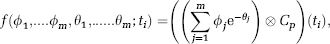
where C_p is the radioligand metabolites-corrected concentration in plasma over time, m the number of tissue compartments in the model, × the convolution operator, and {ϕ₁. …, ϕ _m , θ₁, … .θ _m } the functions of the rate parameters describing movement between compartments.

In the case of a two-tissue compartment model, and in particular of 2TCC,

$f({\varphi }_1,{\varphi }_2,{\theta }_1,{\theta }_2;t_i)=\left(\left(\sum _{j=1}^2{\varphi }_j{\mathrm{e}}^{-{\theta }_j\cdot }\right)\otimes C_p\right)(t_i),$

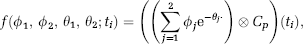
where

$\begin{array}{c}{\theta }_{1,2}\left\{k_2+k_3+k_4\pm \sqrt{(k_2+k_3+k_4{)}^2-4k_2{k}_4}\right\}/2\\ {\varphi }_1=K_1\frac{k_3+k_4-{\theta }_1}{{\theta }_2-{\theta }_1}\end{array}$

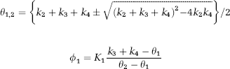
and

${\varphi }_2=-K_1\frac{k_3+k_4-{\theta }_2}{{\theta }_2-{\theta }_1}$

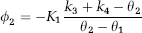
with k₃ and k₄ the fractional rate constants between the intracerebral free plus nonspecifically and specifically bound compartments.

The measurement error ε_i is assumed to be zero mean and independent from the error at other times, with variance var (e_i) = σ²/w_i² described by a generally unknown multiplicative factor σ² and known weights w_i.

Within the framework described in Equation 1, the LS approach computes

$\begin{array}{c}{\mathbf{p}}_{\mathrm{L}\mathrm{S}}={\arg min}_{\mathbf{p}}\sum _{\mathrm{i}=1}^{\mathrm{n}}{\mathrm{w}}_{\mathrm{i}}^2[{\mathrm{y}}_{\mathrm{i}}-\mathrm{f}(\mathbf{p};{\mathrm{t}}_{\mathrm{i}}){]}^2\end{array}$

(2)

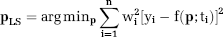
An alternative method for robustly estimating the vector of parameters has been introduced in the study by Koenker and Bassett (1978), for the case of linear QR, and in Koenker and Park (1996), for the extended case of nonlinear QR. The QR estimator is defined by

$\begin{array}{c}{\mathbf{p}}_{\mathrm{Q}\mathrm{R}}={\arg min}_{\mathrm{p}}\sum _{\mathrm{i}=1}^{\mathrm{n}}{\mathrm{w}}_{\mathrm{i}}|{\mathrm{y}}_{\mathrm{i}}-\mathrm{f}(\mathbf{p};{\mathrm{t}}_{\mathrm{i}})|\end{array}$

(3)

and we use the majorize–minimize algorithm of Hunter and Lange (2000) to estimate parameters.

Our reasons for preferring the simple L1 estimator—that is the Lp-norm estimator with p equal to one—include its relative objectivity (beyond the choice of p = 1 for the Lp norm), its simplicity of form, the ready availability of computational routines for performing the fitting, and its low computational costs.

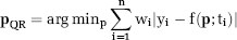
Figure 1 shows the fitted curves obtained by using LS (solid line) and QR (dotted line) to estimate the model parameters in a representative case (i.e., anterior cingulate). The largest gray circle indicates the outlier data point. The two fitting approaches lead to different estimates of the radioligand distribution volume (V_T) for the same considered ROI: 3.50 with LS and 3.35 with QR, respectively. We note that a comparison between the sums of the square residuals obtained by LS and QR, respectively, does not represent a fair measure of the goodness of the fit as, differently from what happens with LS, the (weighted) residual sum of square is not the quantity which is minimized within QR (see Equation 3).

Figure 1

Fitted curves obtained by applying 2TCC with LS (solid line) and QR (dotted line) to model a representative TAC (i.e., anterior cingulate). The gray circles represent the raw TAC data; the largest circle indicates outlier data point.

Outcome Measures and Performance Indices

For each ROI and for all subjects, both LS and QR were applied to fit the TAC to estimate the radioligand V_T as V_T = K₁/k₂(1 + (K₃/k₄)) by considering 2TCC using the Gauss–Newton approach (Coleman and Li, 1994, 1996) for LS. In each subject, the reference region was fitted to a one-tissue compartment and the V_T was always calculated with K₁ and k₂ estimated by LS. Visual inspection of the fitted curves in each subject suggested that the fits obtained by LS and QR were not significantly different for the reference region. The absolute difference between the fitted curves obtained by the two methods for the reference region across subjects and time is in the range from 0 to 0.019. Weights w_i in Equations 2 and 3 were assumed as suggested in the study by Wu and Carson (2002), to include the radioactive decay in modeling the variance for estimating weighting factors. Mean and standard deviation (SD) of V_T values estimated by LS (mean_LS, SD_LS), and QR (mean_QR, SD_QR), respectively, were calculated for each ROI within the group. The mean_QR/mean_LS and SD_QR/SD_LS ratios were then calculated for each ROI.

Results

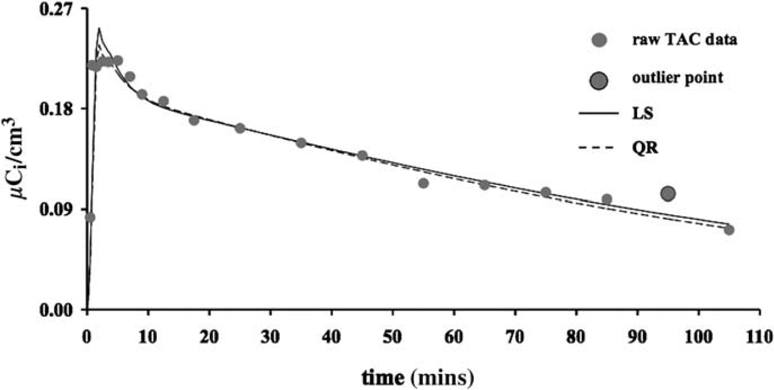
Table 1 reports the summary statistics (mean, SD, and range across all the subjects) of the V_T values estimated by LS and QR in both target and reference regions.

Table 1

Summary statistics (mean, SD, and minimum and maximum across all the subjects) of the V_T values estimated by LS and QR in both target and reference regions

	Mean	s.d.	Min	Max
LS
Raphe nucleus	2.411	0.976	1.152	5.508
Anterior cingulate	3.486	1.225	1.602	7.294
Amygdala	3.604	1.304	1.735	7.761
Cingulate	2.910	1.047	1.324	6.461
Dorsolateral prefrontal cortex	2.920	1.027	1.343	6.417
Hippocampus	5.146	1.917	2.574	10.711
Insula	4.551	1.520	2.226	9.441
Medial prefrontal cortex	3.080	1.028	1.340	6.111
Occipital	2.365	0.863	1.080	5.687
Ventral prefrontal cortex	2.996	1.035	1.351	6.457
Parietal	2.762	0.988	1.298	6.287
Parahippocampal gyrus	4.666	1.598	2.432	9.373
Temporal	3.948	1.340	1.890	8.406
White matter cerebellum	0.293	0.111	0.100	0.624
QR
Raphe nucleus	2.410	0.944	1.152	5.019
Anterior cingulate	3.472	1.190	1.647	6.827
Amygdala	3.578	1.308	1.680	7.749
Cingulate	2.918	1.040	1.380	6.322
Dorsolateral prefrontal cortex	2.917	1.006	1.365	6.174
Hippocampus	5.151	1.930	2.467	10.108
Insula	4.522	1.519	2.255	9.277
Medial prefrontal cortex	3.069	1.026	1.389	6.025
Occipital	2.375	0.849	1.162	5.447
Ventral prefrontal cortex	2.989	1.029	1.329	6.259
Parietal	2.755	0.980	1.328	6.151
Parahippocampal gyrus	4.632	1.591	2.424	8.981
Temporal	3.953	1.350	1.923	8.189
White matter cerebellum	0.292	0.112	0.096	0.641

LS, least squares; QR, quantile regression.

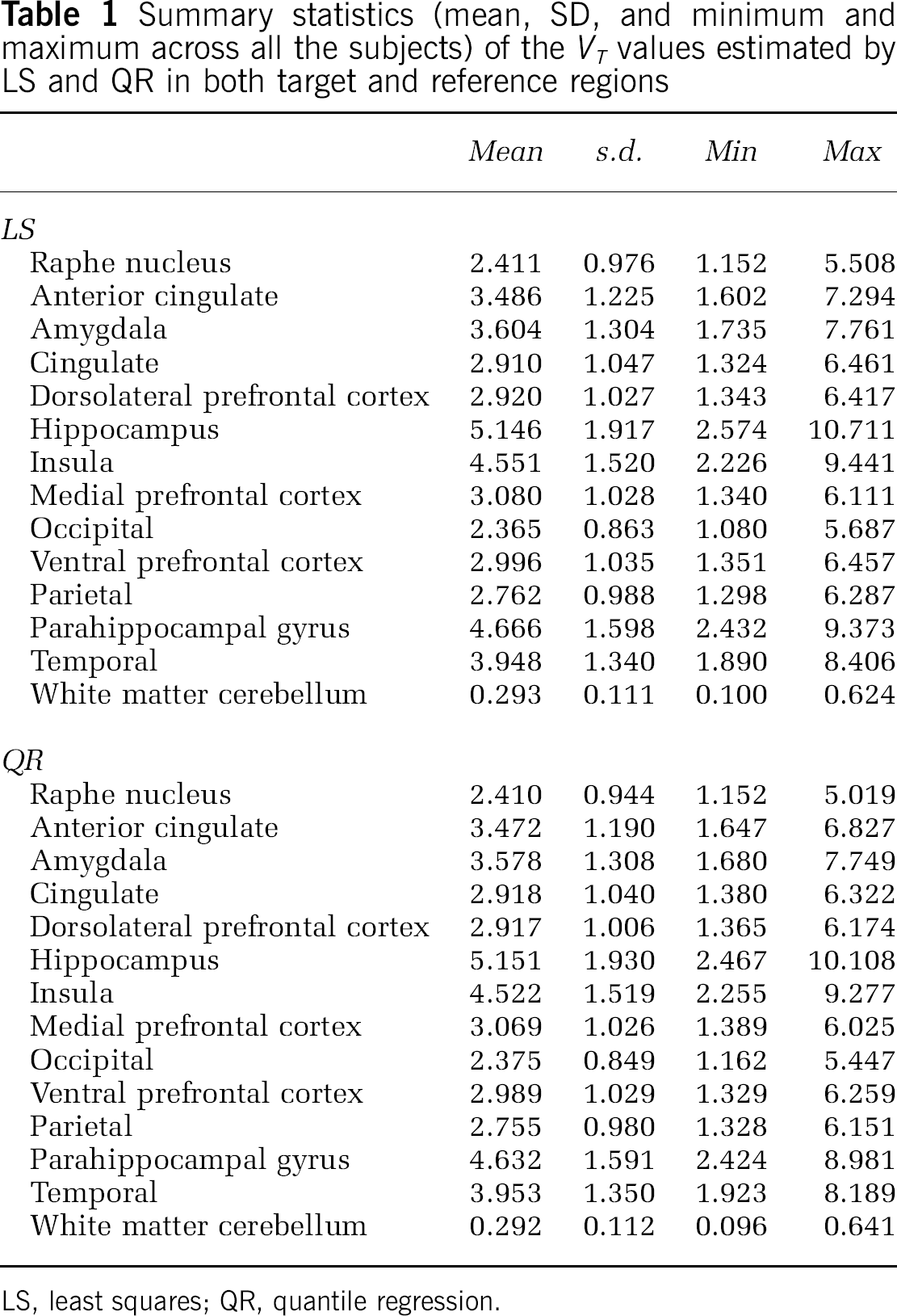
The mean_QR/mean_LS (black solid line) and SD_QR/SD_LS (gray solid line) ratios obtained in each ROI are reported in Figure 2. In terms of SD, the maximum improvement of QR relative to LS is 3.24% (in the raphe nucleus, framed gray box, a region known to be particularly noisy) and the smallest improvement is 0.08% (in the insula, gray box). The mean_QR/mean_LS ratios are close to unity for all ROIs. Relative to LS, QR fails to decrease the SD of estimated V_T in three ROIs (amygdala, hippocampus, and temporal, framed white box). However, in these cases, the increase in the SD observed by applying QR as compared with that by LS (i.e., SD_QR/SD_LS) is overall lower than the decrease obtained in all the other considered ROIs; e.g., in the case of amygdala (SD_QR/SD_LS = 1.0029), only the insula and the medial prefrontal cortex show a decrease in the SD_QR/SD_LS ratios lower than the SD_QR/SD_LS increase in the amygdala (SD_QR/SD_LS = 0.9992 and 0.9984, respectively).

Figure 2

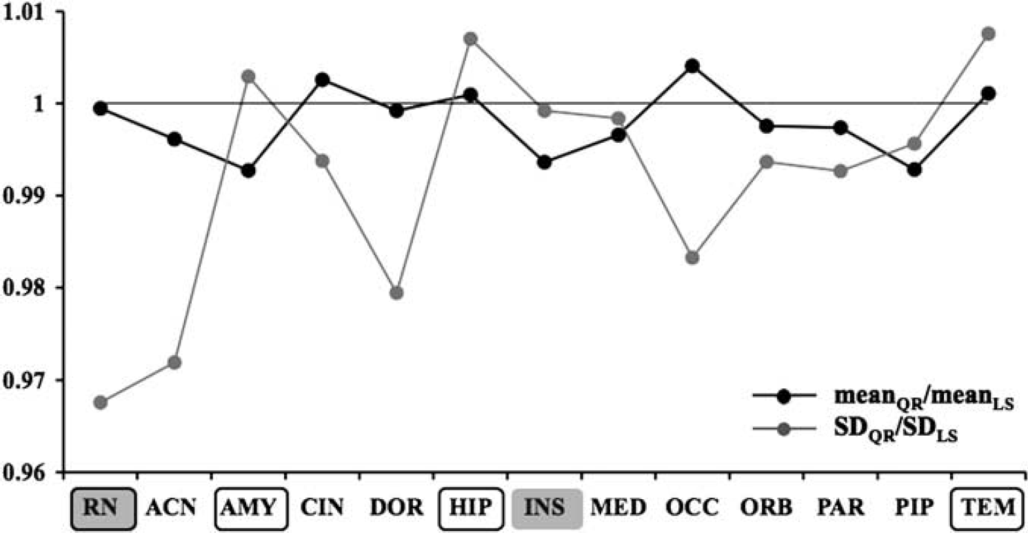
Mean_QR/mean_LS (black solid line) and SD_QR/SD_LS (gray solid line) ratios obtained in 13 ROIs within the [¹¹C]-WAY-100635 group. The framed gray, the gray, and the framed white boxes indicate the best, worst, and failure cases obtained by using QR, respectively. The considered ROIs were: raphe nucleus (RN), anterior cingulate (ACN), amygdala (AMY), cingulate (CIN), dorsolateral prefrontal cortex (DOR), hippocampus (HIP), insula (INS), medial prefrontal cortex (MED), occipital (OCC), ventral prefrontal cortex (ORB), parietal (PAR), parahippocampal gyrus (PIP), temporal (TEM).

Discussion

One potential source of artifacts in PET TAC data is subject head motion that, even with the common use of head fixation devices, cannot be completely eliminated, particularly for some patients. Head motion artifacts can be partially reduced by applying image registration algorithms to the PET data, but these are not capable of correcting within-frame motion, and novel motion tracking systems such as Polaris (Northern Digital, Waterloo, ON, Canada), which would result in smaller problems, have just recently started being introduced during PET scanning sessions and cannot be considered when analyzing previously acquired data. In such a case, QR provides robust estimates that, in contrast to those obtained using LS, are not heavily influenced by outliers.

The results obtained in this study by applying QR to controls studied with [¹¹C]-WAY-100635 show that QR can decrease the SD of V_T estimates across subjects by as much as 3.24%, with an average decrease of 1.24%, at the same time not altering the average estimates of the parameters. This has the effect of improving the statistical power in groups comparisons (or equivalently, reducing the sample size necessary to detect a particular difference). Roughly speaking, a decrease of 3.3% in the SD of the estimated outcome measure will result in a decrease of ∼6% in the number of subjects required to maintain the same power.

We note that there are many sources of variability represented by the variance across subjects of V_T estimates, including biologic differences between subjects, imaging noise, noise in the plasma and metabolite data, uncertainty in modeling each of these sets of data, effects of head motion and other artifacts, as well as subject-to-subject variability. Our aim in this paper is to focus on one relatively small aspect of this total variation—that of errors in the TAC that do not follow a zero-mean Gaussian distribution. Replacing one fitting algorithm with another, as we propose to do, therefore reflects only a relatively small fraction of the overall variability.

One might also argue that nonlinear fitting is not required for a number of PET studies. In fact, for several PET radioligands, the graphical analysis (Logan et al, 1990), which just requires linear fitting, has been widely used (Volkow et al, 1993; Price et al, 2005; Schuitemaker et al, 2007), even though there is a well-known noise-dependent negative bias in the estimation of V_T (Slifstein and Laruelle, 2000). However, for [¹¹C]-WAY-100635, the full input function kinetic analysis with 2TCC, requiring nonlinear fitting, is the method of choice (Parsey et al, 2000).

We also addressed the influence of the weighting factors. We investigated LS and QR performance in the considered data set when alternative weighting templates are adopted by replicating the study assuming weights w_i in Equations 2 and 3 to be the square roots of the time durations of the corresponding PET image frames. With this particular weighting template, the data acquired toward the end have greater weight than those acquired at the beginning of the scan, because emission data are collected as successive frames of increasing duration. The rationale for this weighting scheme is that it gives longer duration frames greater weight, and empirically gives the best performance for this tracer. Furthermore, this weighting scheme has been the weighting template of choice of all the investigations previously published by our laboratory with the [¹¹C]-WAY-100635 radioligand, given that it is less sensitive to the presence of outliers than other templates.

By adopting this weighting template, QR significantly outperforms LS. In particular, QR significantly (p = 0.0001) decreases the SD of the V_T estimates with a relative improvement range of 0.89% (in the insula)—11.20% (in the raphe nucleus), while keeping the within-group average V_T values almost unchanged. To determine the statistical significance of this difference in variance, we selected as our test statistic the average across all ROIs of the variance ratio (SD_QR/SD_LS)². The p-value was determined using a permutation test, randomly permuting the labels (QR/LS) of the estimates for each subject 10,000 times and computing the same test statistic for each permutation (algorithm available upon request). Relative to LS, QR fails to decrease the SD of estimated V_T in just one ROI (amygdala). However, in this case, the increase in the SD observed by applying QR as compared with that by LS (SD_QR/SD_LS = 1.0094) is overall lower than the decrease obtained in all the other considered ROIs; only the insula, in fact, shows a decrease in the SD_QR/SD_LS ratios lower than the SD_QR/SD_LS increase in the amygdala (SD_QR/SD_LS = 0.9911).

We emphasize that all the results reported in this study can be achieved simply by implementing a different fitting approach. We do not mean to suggest that investigators should not perform motion correction, or should not consider the emission-transmission mismatch and the within-frame motion problem, but that after having tried anything that is possible, if outliers are still present in the TACs, the use of QR can help with very low cost.