Comparison of Eight Methods for the Estimation of the Image-Derived Input Function in Dynamic [ 18 F]-FDG PET Human Brain Studies

Abstract

The aim of this study was to compare eight methods for the estimation of the image-derived input function (IDIF) in [¹⁸F]-FDG positron emission tomography (PET) dynamic brain studies. The methods were tested on two digital phantoms and on four healthy volunteers. Image-derived input functions obtained with each method were compared with the reference input functions, that is, the activity in the carotid labels of the phantoms and arterial blood samples for the volunteers, in terms of visual inspection, areas under the curve, cerebral metabolic rates of glucose (CMRglc), and individual rate constants. Blood-sample-free methods provided less reliable results as compared with those obtained using the methods that require the use of blood samples. For some of the blood-sample-free methods, CMRglc estimations considerably improved when the IDIF was calibrated with a single blood sample. Only one of the methods tested in this study, and only in phantom studies, allowed a reliable calculation of the individual rate constants. For the estimation of CMRglc values using an IDIF in [¹⁸F]-FDG PET brain studies, a reliable absolute blood-sample-free procedure is not available yet.

Introduction

Recent years have witnessed a substantial increase of the applications of nuclear imaging techniques, especially positron emission tomography (PET), in different fields of neurology, like neurodegenerative diseases (Brooks, 2008; Mosconi et al, 2008), epileptic disorders (Lee et al, 2009), and brain cancer (Chen and Silverman, 2008). Recently, quantitative PET imaging has been used as a metabolic biomarker to monitor disease progression and to assess the potentially protective effects of drugs (Schmidt et al, 2008; Whone et al, 2003). Positron emission tomography allows the extraction of accurate quantitative information, provided that adequate and specific tracer kinetic models are used. These models often require the assessment of the input function (IF), that is, the tracer concentration over time in arterial plasma. Arterial blood sampling, which is the gold standard for the estimation of the IF, is burdensome and potentially dangerous (Hall, 1971). Time–activity curves obtained from vascular structures on dynamic PET images may provide a less invasive alternative. However, when small brain vasculature is used to obtain an image-derived input function (IDIF), artifacts arising from the limited spatial resolution of PET cameras, that is, spillover and partial volume effect (PVE), must be taken into account.

In the past decade, many different methods aimed at the assessment of an IDIF from internal carotids for PET brain studies have been proposed. Although some of these methods require at least one single blood sample to appropriately scale the image-derived time–activity curve, most efforts have been directed to validate absolutely blood-sample-free procedures.

The aim of the present study was to compare eight previously published different methods for the estimation of an IDIF from dynamic brain PET studies.

Materials and methods

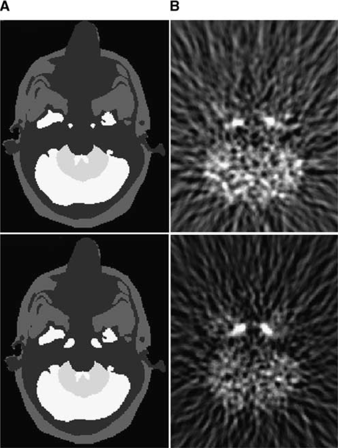
We first compared the different methods using two numerical phantoms of the human brain (Zubal et al, 1994), into which we added two sets of internal carotids, with a diameter of 5 and 8 mm, respectively (Figure 1). The time–activity values associated with the anatomic labels of each brain structure of the phantom were obtained by averaging the tissues values of the four normal subjects included in the clinical study, to obtain ‘typical’ [¹⁸F]-FDG brain pharmacokinetics. Positron emission tomography images were generated using an analytic simulator (Comtat et al, 1999). The different methods were also compared using clinical data from four healthy volunteers.

Figure 1

(A) A transaxial slice of the phantom's head at the level of the carotids. Top row: the phantom with 5 mm diameter carotids. Bottom row: the phantom with 8 mm diameter carotids. (B) An early frame of the reconstructed PET images.

In this section, the characteristics of the phantoms data and clinical studies are first presented. Then, we provide a brief description of each method for the extraction of the IF. All the algorithms are implemented as described in the original articles, except when specifically noted. Finally, we describe the figures of merit used for the comparison of the different techniques.

Phantoms Data

Positron emission tomography images were generated using an analytic simulator that accounts for tomograph geometry, detector arrangement, and detector characteristics (Comtat et al, 1999). The scanner simulated for the study was the ECAT HR+ (Siemens Medical Solutions, Knoxville, TN, USA) used in the three-dimensional acquisition mode. The analytic simulator also includes a four-dimensional smoothing of the projections in the sinogram space to account for the experimentally measured point spread function (PSF) of the scanner. The shape of the four-dimensional smoothing kernel was the sum of two Gaussian functions with variable full width at half maximum (FWHM) to account for variation of the PSF according to the radial position of the lines of response. FWHM and the full width at tenth maximum of the simulated point source were measured according to the NEMA NU 2-2001 protocol. It was, along the radial axis, 4.8 mm FWHM and 9.8 mm full width at tenth maximum at a radial distance of 1 cm, and 6.4 mm FWHM and 12.0 mm full width at tenth maximum at a radial distance of 10 cm.

Each anatomic structure of the human brain phantom (carotids, frontal, temporal, parietal and occipital gray matter, white matter, caudate nuclei, putamens and thalami, bones, and soft tissues) was projected into the sinogram space with the analytical simulator. The dynamic PET acquisition was computed by a linear combination of the projected structures, weighted by the associated kinetics, sampled into time frames, whose number and duration time reproduce exactly those of the clinical studies. Poisson noise was added to the generated sinograms to match the average number of true coincidences measured in the clinical study. Attenuation, random and scattered coincidences were not simulated. The three-dimensional noisy sinograms were rebinned in two dimensional with the FORE algorithm (Defrise et al, 1997) and then reconstructed using the two-dimensional filtered backprojection with a Hann apodization window and a Nyquist cutoff frequency (except where explicitly stated). The voxel size was 1.01 × 1.01 × 2.43 mm³. The 256 × 256 reconstructed slices have a transaxial resolution of 6.8 mm FWHM at the center of the field of view (Figure 1).

Clinical Studies

Four healthy fasting and normoglycemic volunteers underwent a dynamic three-dimensional PET brain scan after injection of [¹⁸F]-FDG (mean activity 140 MBq) on an ECAT HR+ PET machine. The protocol of the study was approved by the local ethical committee. Head movements were minimized using a thermoplastic mask molded individually for each subject. A transmission map for attenuation correction was obtained with external ⁶⁸Ge sources before tracer injection. The acquisition started at the time of the injection and was composed of a dynamic image sequence of approximately 70 mins. The dynamic PET time sequence comprised 12 frames of 10 secs each, 2 × 20 secs, 2 × 150 secs, 5 × 5 mins, 1 × 7 mins, 1 × 10 mins, and 1 × 20 mins. Of note, most of the methods tested in the present study use a minimum frame duration of 10 secs or more in the original papers (Litton, 1997; Naganawa et al, 2005; Su et al, 2005; Parker and Feng, 2005; Mourik et al, 2008a; Zanotti-Fregonara et al, 2007). Image reconstructions were the same as for the phantom studies.

During examination, sequential blood samples from the radial artery were obtained every 10 secs for the first 2 mins, then every 30 secs for the third minute, then at 4, 5, 7, 10, 15, 20, 30, 40, 50, 60, and 70 mins. Blood samples were centrifuged to obtain plasma. The number and the frequency of samples are in the same order of magnitude than those often used in the literature (Phelps et al, 1979; Phillips et al, 1995; Naganawa et al, 2005; Su et al, 2005; Parker and Feng, 2005). The sampling frequency during later times allows obtaining a reliable estimation of the queue of the curve (the most important part for cerebral metabolic rates of glucose (CMRglc) calculation), which is characterized by slow changes in radioactivity levels. Venous plasma samples were also obtained during the last part of the examination using a separate access catheter, to avoid cross-contamination with the injected activity. Each subject underwent a magnetic resonance imaging (MRI) examination as well.

Input Function Extraction Methods

The methods compared in the present study are classified into two groups.

Group A: algorithms that rely on the definition of regions of interest (ROIs) over the carotids arteries. The time activity–curves thus obtained are corrected for PVE.

Group B: algorithms that work without any prior anatomic assumption, in which the carotid time–activity curve is automatically extracted from the voxel kinetics and then scaled to the right amplitude.

Group A

Litton

This method is based on the manual segmentation of carotids on a co-registered MRI study (Litton, 1997). The carotid signal is corrected by a recovery coefficient, assessed experimentally. The spillover from the structures adjacent to the carotids is not accounted for.

In the phantom studies, the anatomic labels of the phantoms were used as MRI-defined ROIs.

For the phantoms, we used a recovery coefficient obtained from the reconstruction of the two sets of carotids labels alone, performed with the same reconstruction parameters as those used for the whole phantom reconstructions. The recovery coefficient obtained from the simulated 5 mm carotids was applied for the clinical studies (Krejza et al, 2006).

Chen et al

The ROIs are manually defined over the carotid arteries on the early PET frames (Chen et al, 1998). The values of the time–activity curves are corrected for the spillover from the surrounding tissue using a manually determined ROI in the vicinity of the carotid ROIs. The measurement from the carotid artery is assumed to be a linear combination of the radioactivity from the blood and from the surrounding tissues:

$$C_{\mathrm{m}\mathrm{e}\mathrm{a}}(t)=\mathrm{R}\mathrm{C}\times C_{\mathrm{p}}(t)+\mathrm{S}\mathrm{P}\times C_{\mathrm{t}}(t)$$

where C_mea is the dynamic data obtained from the carotid ROI, C_p the radioactivity in the blood vessel, and C_t the radioactivity from the surrounding tissues, obtained from the tissue ROI. RC stands for recovery coefficient and SP is the spillover coefficient from tissues to the blood vessel. Using the equation above, the linear least-square method is used to estimate RC and SP at the time points where the measurements for C_mea, C_p, and C_t are available. The measurement of C_p is extrapolated from late venous blood samples. In the phantom studies, the values of activity attributed to the carotid labels are used as surrogate for venous samples. Because venous samplings were not available in each subject, the arterial plasma samples were used in the present study to approximate C_p. Because there is an equilibrium between arterial and late venous blood [¹⁸F]-FDG concentrations, these two can be considered equivalent in the late part of the examination (Chen et al, 1998).

Su et al

Su adopted the approach originally described by Chen et al (1998), but replaced the venous samples with the local frame-wise maximal activity from the carotids (I_max), identified by independent component analysis (ICA), over the first 30 mins of the acquisition after tracer injection (Su et al, 2005). For carotid segmentation, we used the ICA method described by Cardoso and Souloumiac (1993). As proposed by Su, the background tissue ROIs used for PVE and spillover corrections were generated by a dilatation of the blood vessels masks. Final background ROIs were obtained by the difference between the five and three times dilation images (Su et al, 2005).

Parker and Feng

This method also relies on the basic formula described by Chen et al (1998). After reconstruction with an expectation-maximization algorithm, Parker and Feng used the maximum value over the internal carotid ROI (I_max), automatically segmented with the Mumford–Shah algorithm, as an estimate of the reference arterial value (Parker and Feng, 2005). If, at the end of the scan, the surrounding tissue activity exceeds the blood activity, I_max is corrected to I_max × I_mean/T_mean, where I_mean and T_mean are the mean value over the carotid and the tissue background ROI, respectively. In the present study, the 128 × 128 images were reconstructed with an OSEM iterative algorithm using 6 iterations and 16 subsets. The final voxel size was 2.38 × 2.38 × 2.45 mm³. Carotids were automatically segmented with Local Means Analysis algorithm (Maroy et al, 2008).

Zanotti-Fregonara et al

According to the method we proposed in 2007 (Zanotti-Fregonara et al, 2007), carotids are automatically segmented on PET images with Local Means Analysis algorithm (Maroy et al, 2008). Then, 1 cm thick ROIs of the surrounding background tissues are defined by dilatation of the carotid ROIs and PVE correction is obtained using the Geometric Transfer Matrix method (Rousset et al, 1998). In our work, we used the Geometric Transfer Matrix three-dimensional implementation of Frouin et al (2002), in which the regional spread function is obtained by spatial filtering in the image space with a Gaussian kernel, corresponding to the image PSF.

Mourik et al

This approach is based on a reconstruction including a modeling of the tomograph spatial resolution (Mourik et al, 2008a). The reconstruction is based on the normalization and attenuation-weighted OSEM algorithm. The forward projection of the estimated image is convolved with a Gaussian-shaped distribution kernel representing the PSF of the system. After a reconstruction performed with 4 iterations and 16 subsets, Mourik et al obtained the IFs by averaging the four hottest pixels per plane within the carotids, from 15 to 45 secs after injection. In the present work, reconstructions were performed using the PSF in the forward projection only, as in the original paper of Mourik, and with the complete PSF modelization as well.

Group B

Naganawa et al

Naganawa et al (2005) used an approach based on the ICA. They used the principal component analysis as a first step to reduce the dimensions of the dynamic PET image sequence to two and apply fixed-point algorithm for ICA to extract kinetics. EPICA, the version of ICA they used, which includes specific properties of the human brain [¹⁸F]-FDG data, is freely available at http://home.att.ne.jp/lemon/mikan/EPICA.html. Time–activity curves are extracted without any anatomic assumption and effects of spillover are implicitly accounted for through the source signal mixing process. Of note, the kinetics must be normalized because of indeterminacy in the ICA problem. The authors proposed to adjust the scale of the estimated time–activity values by one-point arterial blood sampling, taken at the peak of the plasma time–activity curve. In our phantom studies, the activity in the carotid anatomic label is used as surrogate of arterial blood activity concentration.

Bodvarsson et al

Nonnegative matrix factorization (NMF) is used to extract the tracer kinetics from PET four-dimensional images (Bodvarsson et al, 2006). The proposed technique is called multiplicative update (Lee and Seung, 1999) and minimizes the squared Euclidean distance between the matrix V, and the linear combination of the factors W and H, that is, V=WH, where V is the dynamic PET image, W the mixing matrix, and H contains the basis time–activity curves. All elements in V, W, and H are nonnegative. We estimated the time–activity curves using two and three sources. The scaling of the estimated curves is performed using an α factor (Bodvarsson and Mørkebjerg, 2006), found by making assumptions on W. Because W describes the contribution of each component in each voxel, it can be assumed that the sum equals 1 in all voxels. A Matlab implementation of this rescaling is provided at http://isp.imm.dtu.dk/toolbox/nmf.

Figures of Merit Used for the Comparison of the Different Techniques

Visual analysis

Partial volume effect corrected carotid time–activity curves obtained with each method were visually compared with the reference values, that is, the time–activity curves composed by the original values in the carotid anatomic labels in the phantom studies and arterial blood sampling for the volunteers.

Comparison of the areas under the curve

In both simulated and clinical data, the areas under the curve (AUCs) obtained with each technique were compared with the reference AUCs in terms of mean relative difference.

CMRglc calculation

Cerebral metabolic rates of glucose values were calculated with the Patlak analysis (Patlak et al, 1983). The lumped constant was set at 0.65 (Wu et al, 2003). For the phantom studies, CMRglc values were obtained for 20 different anatomic labels of the phantom brain. For clinical studies, CMRglc were calculated on 62 different brain regions, defined on the superimposed MRI of each healthy volunteer. CMRglc values obtained using the arterial blood samples were considered as the reference values. A linear regression was used to compare the reference values with the values calculated with each method. A score system (ranging from 0 to 12 points) is used to compare the different methods. The test–retest variability for brain CMRglc is usually less than ±5%. Higher figures have been reported, but they are usually comprised between ±10% (see Schmidt et al, 1996 for a review). Using the linear regression, with no intercept, results of the phantoms and clinical studies we attributed a score of 2 each time a method provided a CMRglc estimation comprised between +5% and −5% as compared with the reference values, a score of 1 if comprised between ±5% and 10%, and a score of 0 if higher than ±10%.

Impact of scaling with a blood sample

For those methods that theoretically do not require blood sampling, that is, Litton, Su, Parker and Feng, Zanotti-Fregonara, Mourik and Bodvarsson, CMRglc values were calculated also after calibration of the IDIF with a single plasma sample, taken 30 mins after injection.

Individual rate constants calculation

Both in clinical and phantom studies, the individual rate constants (K₁, k₂, and k₃) were calculated for each method, using the classical three-compartment FDG model (Phelps et al, 1979). Results were compared with the reference rate constants in terms of mean percentage variation.

There is always a slight time-shift between the image-derived carotid time–activity curves and the measured plasma samples from radial arteries. Although this difference is negligible for the estimation of CMRglc (Guo et al, 2007), it could indeed influence the quantification of individual rate constants. Therefore the plasma curves were shifted to match the image-derived carotid curves.

Results

Visual Analysis and Comparison of the Areas Under the Curve

Figure 2 shows the IDIF curves, calculated with the different methods, in one of the subjects for each method. Similar results were obtained for each subject and in the two phantoms.

Figure 2

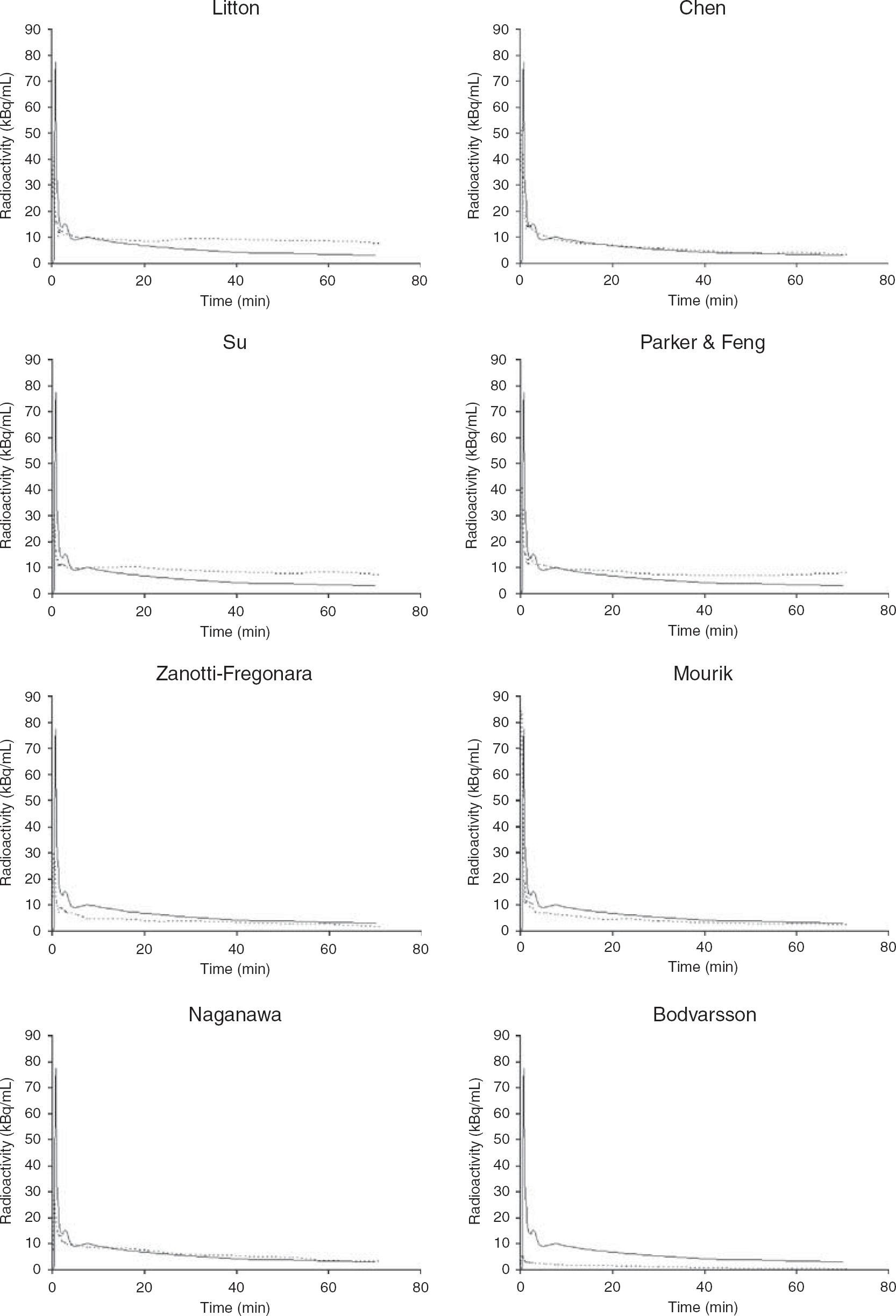
IDIF estimation in one subject with the different methods. The curves of Bodvarsson, Zanotti-Fregonara, and Mourik are those not calibrated with a blood sample. Solid line, reference IF; dotted line, estimated IF.

Methods of Group A

Litton

In our simulated data, the ideal recovery coefficient was estimated at 0.45 for the 8 mm phantom and 0.21 for the 5 mm phantom. The early part of the curve (first 4 to 5 mins), where the spillover from surrounding tissues into the artery ROIs is small, was correctly estimated in both phantoms. However, there was a progressive overestimation of the tail of the curve, which led to a mean AUC overestimation of +60.6%. In the clinical studies, although the peaks were underestimated in the four subjects, we also observed an overestimation of the tails of the curves. The subjects’ image-derived IFs gave a mean overestimation of the AUCs of +17.2%.

Chen et al

For both phantoms, the visual inspection showed an excellent correlation between the reference and the estimated time–activity curves, with a mean AUC difference from the reference curve that did not exceed 2%. In all the clinical studies, the maximum of the peak was underestimated as compared with the arterial peak. However, as compared with the reference curves, the width of the peak was very similar and the tail of the image-derived curves coincided well. The image-derived AUCs of the clinical studies yielded a small mean underestimation of −7.6%.

Su et al

In both phantoms, the visual analysis of the curves showed an underestimation of the early peak. Conversely, the tails of the curve were overestimated (mean estimated AUC: +33.6%). The same pattern was observed in three of the four subjects. In the last one the AUC was slightly underestimated (−7.2%). The mean estimated AUC for the four subjects was +11.7%.

Parker and Feng

In both phantoms and in each volunteer, the background activity concentration at the end of the scan exceeded the activity concentration in the carotid, so that I_max had to be corrected in all cases. The visual analysis shows that the estimated IF for the 8 mm carotid phantom underestimated the peak and overestimated the late part of the curve (estimated AUC: +53%). Conversely, in the 5 mm carotid phantom, we observed an underestimation of both the peak and the tail of the curve (AUC mean relative difference: −44.6%). Variable results were observed for the clinical studies. In one of the subjects the IDIF matched quite well the reference IF (AUC: −7.6%), but in the other three the AUC was largely overestimated because an elevated tail of the IDIFs (mean AUC in the four subjects: +40.3%).

Zanotti-Fregonara et al

The early part of the IDIFs was underestimated in the two phantoms and in each of the healthy volunteers. Although the shape of the tails reproduced well that of the reference curve, they were underestimated in both phantoms and in three of the four volunteers. The mean AUC was −48.8% for simulated data and −35% for clinical data.

Mourik et al

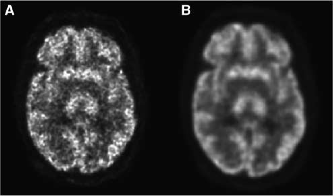
In both phantom and clinical studies, the images reconstructed including the PSF in both forward and back projection were of better quality as compared with those obtained using a reconstruction with the PSF modeled in the forward projection only (Figure 3). Therefore, IDIFs were estimated using the images reconstructed with the complete modelization of the PSF. Using the noncalibrated curves, we observed an overestimation of the peak in both phantoms. Although the shape of the tails reproduced well that of the reference curve, they were underestimated in both phantoms. The resulting AUCs were lower as compared with the reference AUC (mean: −34%). A similar aspect was observed in the clinical studies (mean AUC: −36.3%).

Methods of Group B

Naganawa et al

In the 8 mm carotid phantom, the AUC of the estimated IF matched very well the reference AUC (difference: −1.7%). However, for the 5 mm phantom we were unable to obtain an IF-like time–activity curve. As compared with the 8 mm carotid phantom, the shape of the curve in each of the subjects was not as well estimated as that of the phantom. In particular, we observed underestimated peaks and slower descending slopes. Therefore, the normalization of the estimated curves using the arterial peak, as proposed by Naganawa et al (2005), would have given largely overestimated IFs. Thus, we performed the normalizations by using a blood sample at 30 mins from the injection. Although the peak was underestimated in each subject, the last part of the estimated IF matched quite well the reference curve in the four volunteers. The mean estimated AUC was −18.6% as compared with the reference AUCs.

Bodvarsson et al

We were unable to extract an IF-like time–activity curve in the 5 mm phantom. The shape of the IF we obtained in the 8 mm phantom was quite different from the shape of the reference curve: although the tails of the curves were roughly similar, the curve obtained by NMF showed a very low peak. After scaling this curve using the α factor proposed by the authors (Bodvarsson and Mørkebjerg, 2006), we obtained a largely underestimated IF (AUC: −90.7%). In the four subjects the shape of the curves was poorly estimated as well and the scaling with the α factor gave similar results as those of the phantom (mean AUC: −80.5%). No significant differences were observed by using two or three sources.

CMRglc Calculation

Table 1 shows the linear regression results of the CMRglc values estimated by the different IDIFs, compared with the reference values, in the phantoms and in the four subjects, respectively.

Table 1

Results of CMRglc values in the two phantoms and the four healthy volunteers

Method	Phantom with 8 mm carotids		Phantom with 5 mm carotids		Subject 1		Subject 2		Subject 3		Subject 4		Score
Litton	0.814x+0.55	0.828x	0.298x−0.34	0.290x	0.667x−1.21	0.599x	0.501x−1.79	0.410x	0.449x−1.61	0.382x	0.721x−2.54	0.596x	0
Chen	0.980x−0.03	0.979x	1.027+0.24	1.036	0.975x+0.06	0.978x	0.967x+0.44	0.989x	1.073x−0.77	1.041x	1.047x−0.40	1.027x	12
Naganawa	1.078x+0.07	1.079x	—	—	1.006x−0.54	0.976x	1.008x+0.01	1.008x	0.957x−1.32	0.898x	1.205x+0.65	1.238x	5
Su	0.333x−0.04	0.332x	0.299x−0.70	0.281x	0.627x−0.32	0.608x	0.556x−1.69	0.471x	0.845x−1.67	0.775x	0.766x−0.40	0.746x	0
Parker and Feng	0.252x−0.02	0.251x	1.75x−3.59	1.653x	0.926x+1.05	0.985x	0.581x−1.91	0.483x	0.356x−0.88	0.319x	0.519x−0.79	0.480x	2
Bodvarsson a	4.634x−8.84	4.856x	—	—	8.103x+6.38	8.461x	6.370x+23.1	7.627x	5.676x+13.1	6.227x	3.149x+5.61	3.426x	0
Bodvarsson b	1.439x−1.80	1.370x	—	—	1.118x−0.87	1.167x	1.058x+3.12	1.222x	0.971x+1.37	1.029x	1.112x+3.17	1.268x	2
Zanotti-Fregonara a	1.372x+0.14	1.376x	2.196x−0.53	2.182x	1.450x+1.14	1.514x	1.328x−0.08	1.324x	0.986x−2.31	0.889x	1.591x−0.01	1.590x	2
Zanotti-Fregonara b	1.041x−0.50	1.021x	1.089−0.27	1.078x	1.077x+0.97	1.132x	1.117−0.06	1.113x	0.914x−2.17	0.823x	1.081x−1.32	1.016x	5
Mourik a	1.248x−0.88	1.225x	2.374x−0.72	2.355x	1.747x+1.36	1.823x	1.333x+2.58	1.474x	1.120x+5.45	1.348x	1.521x+6.91	1.863x	0
Mourik b	1.038x+0.46	1.056x	1.146x−0.51	1.133x	0.998x+0.70	1.037x	1.034x−0.16	1.026x	0.950x−0.34	0.935x	1.024x+0.38	1.047x	8

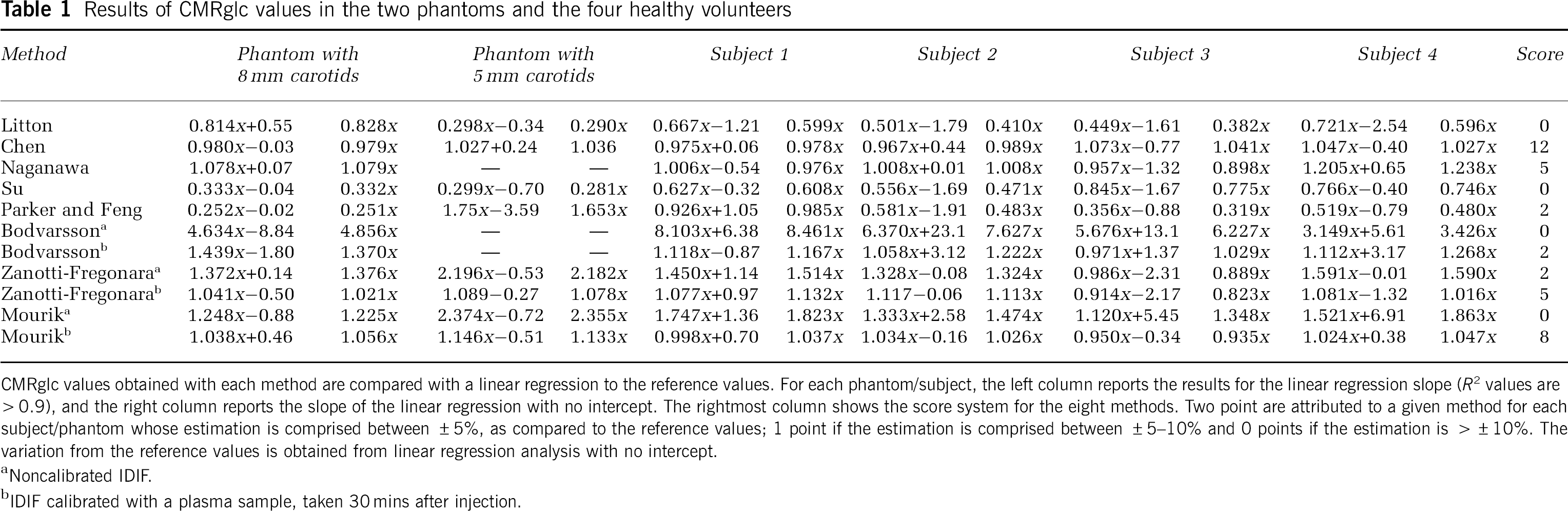
CMRglc values obtained with each method are compared with a linear regression to the reference values. For each phantom/subject, the left column reports the results for the linear regression slope (R² values are >0.9), and the right column reports the slope of the linear regression with no intercept. The rightmost column shows the score system for the eight methods. Two point are attributed to a given method for each subject/phantom whose estimation is comprised between ±5%, as compared to the reference values; 1 point if the estimation is comprised between ±5–10% and 0 points if the estimation is >±10%. The variation from the reference values is obtained from linear regression analysis with no intercept.

a

Noncalibrated IDIF.

b

IDIF calibrated with a plasma sample, taken 30 mins after injection.

Figure 3

(A) A transaxial slice of a brain phantom reconstructed by an analytic simulator with the Point Spread Function included in the forward projection only (B) the same slice with the complete modelization of the Point Spread Function.

Very good results were obtained with the method of Chen (score: 12), both in phantom and in clinical studies. Contrarily so, with the method of Su, we obtained underestimated CMRglc values (score: 0). To assess whether the use of I_max or the use of automatic circular background ROIs could explain the differences in the results obtained with these two methods, we corrected PVE in the phantoms of Su (those with automatic circular background ROIs) using plasma samples, as proposed by Chen. The results of linear regression changed from 0.3327x−0.0365 to 1.007x−0.0202 for the 8 mm phantom and from 0.2992x−0.7001 to 0.9665x+0.0084 for the 5 mm carotid phantom. These data suggest that errors in CMRglc estimation using the method of Su were not linked to the methodology of background ROIs definition.

Impact of Scaling With a Blood Sample

In three blood-sample-free procedures, that is, those of Litton, Su, and Parker and Feng, the calibration could not be reliably performed. Indeed, the spillover from surrounding tissues often entails a progressive increase of the late part of the curve, thus precluding a reliable correction on the basis of a single blood sample.

Although results improved after calibration with a blood sample for both the methods of Zanotti-Fregonara (score: 5) and Bodvarsson (score: 2), the estimation of CMRglc values was still less precise than that obtained with other methods.

Better results were obtained with the method of Mourik (score: 8).

Individual Rate Constants Calculation

Table 2 shows the results of the estimation of the individual rate constants in the clinical studies, calculated with each method and compared with the reference constants obtained by arterial blood sampling. Large and unpredictable under- and overestimations were observed in each subject and using each method.

Table 2

Results of individual rate constants calculations (mean±standard deviation) in the four subjects for each method and variation in percentage from the reference values

	Mean K 1	Variation %	Mean k 2	Variation %	Mean k 3	Variation %
Arterial samples	0.0960±0.0198		0.1086±0.0121		0.0416±0.0012
Litton	0.1746±0.0330	+82	0.1885±0.0613	+73.6	0.0172±0.0047	−58.7
Chen	0.1467±0.0627	+52.9	0.1806±0.0906	+66.4	0.0426±0.0115	+2.4
Naganawa	0.1619±0.0344	+68.7	0.0808±0.0256	−25.6	0.0234±0.0118	−43.8
Su	0.1676±0.0440	+74.7	0.1960±0.0394	+80.5	0.0277±0.0104	−33.4
Parker and Feng	0.1090±0.0305	+13.6	0.1437±0.0336	+32.3	0.0264±0.0078	−36.7
Bodvarsson a	0.2879±0.3103	+200	0.1733±0.0602	+59.6	0.0623±0.0274	+49.7
Zanotti-Fregonara a	0.1427±0.0384	+48.7	0.0794±0.0564	−26.9	0.0224±0.0183	−46.3
Mourik a	0.0737±0.0077	−23.2	0.0760±0.0161	−30.1	0.0372±0.0101	−10.7

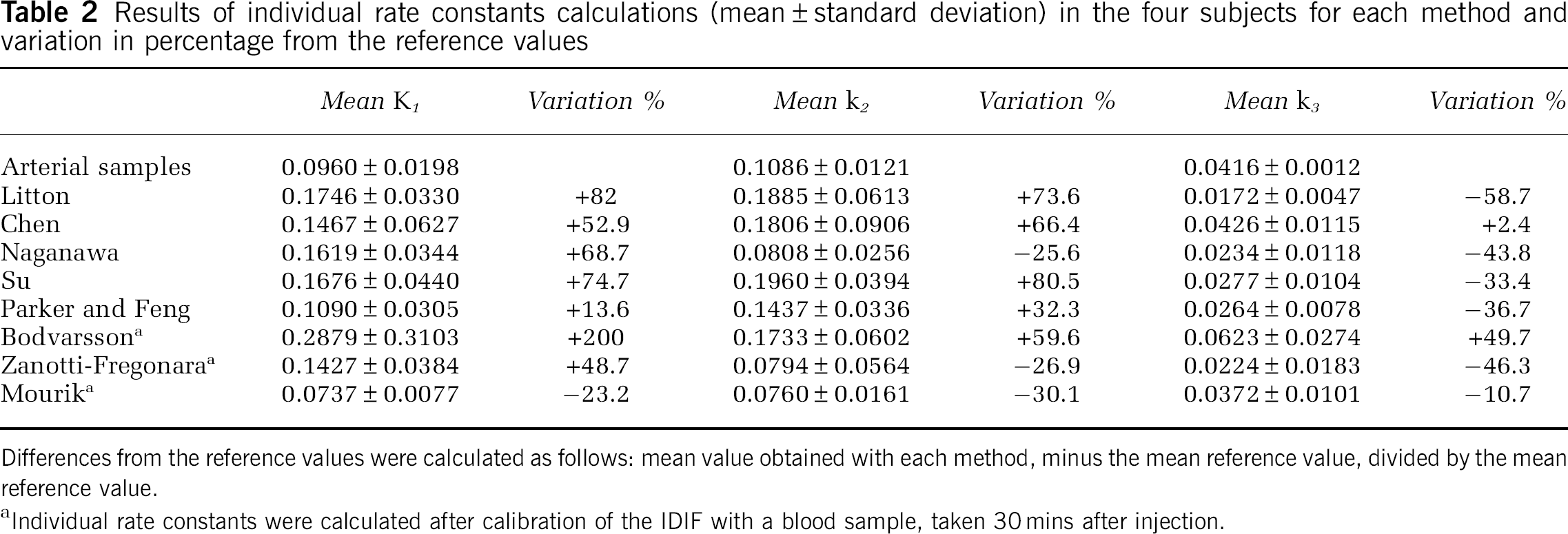
Differences from the reference values were calculated as follows: mean value obtained with each method, minus the mean reference value, divided by the mean reference value.

a

Individual rate constants were calculated after calibration of the IDIF with a blood sample, taken 30 mins after injection.

Individual rate constants were then calculated for phantom studies. Excellent results were obtained with the method of Chen (mean variation in percentage: +1.2%, +2.7%, and +2.7% for K₁, k₂, and k₃, respectively). Although partial improvements, as compared with clinical data, were sometimes observed, large over- and underestimations are obtained with all the other methods (data not shown).

Discussion

In the present study, we compared eight different techniques aimed at obtaining useful IDIFs in dynamic [¹⁸F]-FDG PET brain studies.

Besides using images from real subjects, there are three main reasons why we chose to test the different methods on digital phantoms as well. (1) Phantom studies allow knowing the precise concentration of radioactivity in carotid arteries. This concentration is not affected by possible arterial blood measurement errors. Moreover, phantom IFs do not have delay and dispersion and the height of the early peak is known exactly. (2) The phantoms IDIFs are not affected by temporal PET sampling, as each frame corresponds to a punctual detection at a given time; that is, the temporal sampling is ‘ideal’. (3) Clinical studies may have slight movements of the patient's head.

These biases probably explain the discrepancies that we have sometimes found between the results of phantom and clinical studies. For example in the phantom studies, the AUCs obtained with the method of Chen matched very well the reference IFs (differences <2%) and the height of the peak was estimated precisely. When the same methods were applied to clinical studies, we obtained a mean AUC underestimation of −7.6%. These variations are almost exclusively the consequence of the underestimation of the early part of the curve, because the averaging of the signal over each PET frame. It is expected that a finer temporal PET sampling (ideally a list-mode acquisition) would allow obtaining results closer to those of the phantoms.

In the present study, excellent results for CMRglc estimation, both in phantom and clinical data, were obtained using the method described by Chen et al (1998) (score: 12). This technique is however the most invasive among those we tested, as it requires at least three venous blood samples.

Using the method proposed by Litton (1997), we observed an overestimation of the late portion of the curve in each subject and in both phantoms, which translated into an underestimation of CMRglc values. These data point to the necessity of implementing an adequate correction not only for PVE, but also for spillover artifacts from the surrounding brain tissues. Besides the need of performing another examination, approaches that rely on a co-registered MRI may be prone to errors because misalignment artifacts. Co-registration software are based on brain structures, whereas carotids are located outside the brain. The carotids are elastic structures that may undergo complex deformations in case of even a slight difference in patient positioning between PET and MRI studies. Finally, the co-registration quality can also be hampered by distortions because of magnetic susceptibility variations (Sumanaweera et al, 1994).

Using the method of Su et al (2005), we observed an underestimation of the peak and an overestimation of the tails of the curves in both phantoms. Except in one volunteer, similar findings were obtained in the other three subjects. The elevation of the curve tail is most likely due to an underestimation of the tissue spillover into carotids, because of a lower uptake by brain tissue at the early part of the examination. The results we found using the method of Su et al (2005) are in agreement with those reported by other authors (Chen et al, 2007).

Most of the curves obtained with the method of Parker and Feng (2005) showed a progressive increase of the last part, which suggests that this method does not allow a precise correction of the spillover from surrounding tissues. We automatically segmented the carotids using the Local Means Analysis algorithm (Maroy et al, 2008), instead of the Mumford–Shah based algorithm used in the original paper (Parker and Feng, 2005). However, it is unlikely that this could have influenced the magnitude of the results. Indeed, Local Means Analysis provides excellent performances for internal carotids segmentation in dynamic PET studies (Zanotti-Fregonara et al, 2009). Moreover, the maximum value inside the carotid ROIs, required to perform PVE correction according to the procedure of Parker and Feng, is usually located in the middle of the carotids and does not change over different segmentation methods.

In 2007, we proposed a method that relies on the Geometric Transfer Matrix algorithm to correct spillover and PVE in the carotids (Zanotti-Fregonara et al, 2007). Our results show that this method corrects well the spillover effect, because the shape of the tails of the curves reproduced well the reference curves. However, this method does not allow a complete correction for PVE and a calibration with a blood sample is necessary to improve CMRglc estimation. Even after calibration, our method is less precise (score: 5) and technically more complicated as compared with other methods.

In the present work, the method of Mourik et al (2008a) is applied to [¹⁸F]-FDG studies for the first time. Using this method without calibration of the IDIF, we observed a certain degree of underestimation of the curve tail in both phantoms and in each of the clinical studies, which entailed an overestimation of CMRglc values. Calibration greatly improved the estimation of the CMRglc values (score: 8). Mourik et al (2008a, 2009) tested their method on four different tracers and found that calibration is not necessary for either (R)-[¹¹C]verapamil or [¹¹C]flumazenil, but it is essential for [¹¹C]PIB and preferred for (R)-[¹¹C]PK11195. In fact, different tracers show different activity uptake, distribution, and contrast, resulting in a differential scatter distribution (Mourik et al, 2009). Of note, calibration becomes necessary for [¹¹C]flumazenil studies when acquired on a High Resolution Research Tomograph (Mourik et al, 2008b). This suggests that the necessity of calibrating the IF estimated with this method should be carefully assessed for each tracer and for each machine. Further studies are necessary to assess whether reconstruction-based PVE-corrected images using higher-resolution tomographs (Sureau et al, 2008) may allow a reliable estimation of [¹⁸F]-FDG IDIFs without the need of blood sampling.

Using the method of Naganawa et al (2005), we were unable to extract an IF-like time–activity curve in the 5 mm phantom. The most likely explanation is that the number of voxels containing ‘vascular’ kinetics in this phantom is too small to provide a detectable signal. This problem does not exist in the clinical studies, where almost every brain voxel contributes to the vascular signal. The shapes of the estimated curves we obtained in the four clinical subjects were not as good as that we found for our 8 mm carotid phantom. This could be partly because of the fact that the time–activity vascular curves extracted without any anatomic assumption over the whole brain include both arteries and veins. The resulting time–activity curve is unlikely to match exactly the shape of a pure arterial plasma IF. To adjust the amplitude of the curves obtained by ICA, Naganawa used an arterial blood sample at the peak. However, this could be not the optimal choice in the clinical practice, because the height of the peak would inevitably be averaged over the frame duration. Indeed, the normalization of the subjects’ IDIFs with the peak arterial sample would have given a large overestimation of the curves. Thus, we chose a late blood sample (at 30 mins) as a normalization factor. Because there is tracer equilibrium of ¹⁸F-FDG concentration between arterial and venous blood at late times (Chen et al, 1998), a late venous blood sample would produce less invasive and more robust results than an early arterial blood sample.

Using the nonnegative matrix factorization (Bodvarsson et al, 2006), we could not generate an IF-like curve in the 5 mm carotid phantom, probably because of the same problem of sensitivity encountered in this phantom using the segmentation with ICA. The shape of the IFs extracted from the images of the 8 mm carotid phantom and of the four subjects did not match well the reference curves, in particular because of very flat peaks. After the scaling of the curves with the α factor (Bodvarsson and Mørkebjerg, 2006), we obtained much underestimated curves in both simulated and clinical data, and the resulting AUCs were inconsistent with the reference AUCs. After scaling the curves using a blood sample, the CMRglc estimations partially improved (score: 2). Incidentally, it should be noted that Bodvarsson uses the algorithm of Lee and Seung (1999), which is easy to implement but suffers from the existence of local minima, and the use of random matrix to initialize the algorithm can make the algorithm converge to these minima, in particular in noisy PET images.

In the absence of blood samples, the correct scaling of the late part of the image-derived curves becomes a difficult task. Indeed, none of the totally noninvasive methods evaluated here could completely correct the PVE of the carotid time–activity curves. Therefore, our results suggest that late blood samples should be obtained whenever possible. It should be noted that venous blood sampling is an accurate way to obtain blood glucose concentration, which is required for CMRglc quantification. Toward the end of a typical [¹⁸F]-FDG brain examination, the high [¹⁸F]-FDG uptake of the brain gray matter entails an important spillover into the carotid ROIs. When spillover correction is not performed (Litton, 1997) or performed imprecisely (Su et al, 2005; Parker and Feng, 2005) the progressive increase of the apparent activity within the carotid ROIs precludes the possibility of a reliable correction by blood sampling.

The evaluation of the basic mechanisms of regional glucose metabolism by estimating forward and reverse glucose transport (K₁ and k₂) as well as the initial intracellular metabolic step, the phosphorylation of [¹⁸F]-FDG by hexokinase (k₃), may be more sensitive markers of disease progression than CMRglc values. When using an IDIF, a poor estimation of the early part of the curve is usually a relatively minor problem for the estimation of CMRglc with the Patlak method. However, individual rate constants are much more sensitive to variations in the shape of the early part of the curve. In our clinical data, a huge amount of uncertainty in their calculation was found with each method. The arterial IFs of the four subjects were not corrected for dispersion; however, the extent of this dispersion should be very limited and should not explain the large errors in the estimation of individual constants. More probably, estimation errors are mostly because of the PET temporal resolution artifacts. Of note, phantom data do not suffer from artifacts due to IF delay, dispersion, temporal PET framing, and blood radioactivity measurement errors.

Our phantom data suggest that the only method that could potentially estimate the individual constants is that of Chen. Further studies with a more rapid PET framing (ideally with a list-mode acquisition) and dispersion correction are necessary to assess whether this method could allow a reliable estimation of microparameters using clinical dynamic PET images.

Conclusion

For the estimation of CMRglc values using an IDIF from carotid arteries in [¹⁸F]-FDG PET brain studies, our data suggest that a reliable absolute blood-sample-free procedure is not available yet. Late venous blood samples should be obtained whenever possible.