Modeling Considerations for In Vivo Quantification of the Dopamine Transporter using [ 11 C]PE2I and Positron Emission Tomography

Abstract

The dopamine transporter (DAT) is an important imaging target as changes in DAT have been implicated in a variety of neurologic and psychiatric disorders and can result from certain classes of medications. [¹¹C]N-(3-iodoprop-2E-enyl)-2β-carbomethoxy-3β-(4-methylphenyl)nortropane ([¹¹C]PE2I), a radioligand with high specificity for DAT, has been shown to exhibit favorable kinetics and to produce high contrast positron emission tomography (PET) images. To better characterize this ligand and to assess its measurement reliability, PET images of seven subjects were acquired in a test–retest paradigm. For optimal model performance, each subject was scanned for 120 mins, ensuring that high binding regions could reach equilibrium, a validated coregistration method was performed for accurate anatomic delineations and an exhaustive search for a reference region having one-tissue compartment kinetics was undertaken. Eleven modeling methods were tested and six metrics were used for method evaluation. A noniterative two-tissue compartment method with 100 mins of scanning time was found to be optimal for characterizing [¹¹C]PE2I.

Introduction

The dopamine transporter (DAT) is a presynaptic, membrane-spanning protein that binds to dopamine for reuptake (Hall et al, 1999; Halldin et al, 2003; Jucaite et al, 2006; Drewes et al, 2007). It is found mainly, although not exclusively, in the striatum and is necessary for regulation of dopamine concentration; and therefore, for termination of the dopamine signal (Kuikka et al, 1998; Halldin et al, 2003; Drewes et al, 2007). Altered DAT availability has been implicated in alcoholism, depression, attention-deficit-hyperactivity disorder, neuropsychiatrie disorders, and in neurodegenerative diseases (Guilloteau et al, 1998; Kuikka et al, 1998; Halldin et al, 2003; Jucaite et al, 2006; Leroy et al, 2007; Ziebell et al, 2007). As DAT loss may precede clinical symptoms in some diseases, such as idiopathic Parkinson's disease (Leroy et al, 2007), imaging this transporter could be an especially helpful diagnostic indicator (Herholz, 2004; Ziebell et al, 2007). Dopamine transporter imaging could also aid in evaluating the neuroprotective effects of new pharmaceuticals.

Owing to its selectivity for DAT and favorable kinetics, the radioligand N-(3-iodoprop-2E-enyl)-2β-carbomethoxy-3β-(4-methylphenyl)nortropane (PE2I) can be a valuable tool for DAT imaging (Halldin et al, 2003; Jucaite et al, 2006; Hirvonen et al, 2008). In competition studies, PE2I showed high affinity for DAT in vitro (K_i, = 17 nmol/L) with a significantly lower binding affinity for serotonin or norepinephrine transporters (Emond et al, 2008). In vitro saturation studies have also validated the high DAT affinity of PE2I, resulting in a measured (Na + dependent) K_d of 3.9 nmol/L in 120 mmol/L of NaCl (Emond et al, 2008). However, DAT measurements using PE2I have shown great variability (Jucaite et al, 2006; Leroy et al, 2007). To examine the source of this interindividual variability, a test–retest paradigm is needed.

Initial test-retest studies carried out by Hirvonen et al (2008) yielded promising results. However, in those studies, the high binding striatal regions had not reached equilibrium within the 69 mins of scanning time. This prevented modeling of the time activity curves (TACs) using graphical methods (as a linear part of the Logan integral graph could not be obtained) and may have affected the estimation of outcome measures in the high binding regions. In addition, the coregistration between positron emission tomography (PET) images and magnetic resonance images (MRIs) was based on minimizing a mutual information-type cost function, as is often the case (Leroy et al, 2007; Hirvonen et al, 2008; Ito et al, 2008). However, recent work (DeLorenzo et al, 2009) has shown that a single coregistration technique may not be optimal in all cases and that coregistration inaccuracies can yield up to 20% error in calculated outcome measures.

To address these problems, in this study, subjects were scanned for 120 mins, allowing the high binding regions to reach equilibrium. The extra scanning time expanded the modeling possibilities, allowing the use of graphical approaches. Moreover, eight possible coregistrations were performed for each PET acquisition, and the optimum coregistration was automatically chosen on the basis of a technique that has been extensively tested.

To improve the accuracy of reference tissue approaches, efforts were made to determine a suitable reference region. As most reference methods assume that a one-tissue compartment (1TC) model describes the reference region, clustering techniques were used to isolate possible regions of the brain that meet this criteria.

Materials and methods

Subjects

Seven healthy volunteers (five women, two men; mean age 32 ± 9 years, range 25 to 45 years) were recruited for this study. All subjects were nonsmokers. Inclusion criteria were assessed by the following: history, Structured Clinical Interview for the Diagnostic and Statistical Manual of Mental Disorders IV (SCID), review of systems, physical examination, routine blood tests, pregnancy test, urine toxicology, and electrocardiography. The inclusion criteria consisted of (1) age 18 to 50 years, (2) no significant medical illness on physical examination, (3) no Axis I diagnosis on the basis of the SCID, (4) negative pregnancy test for women, (5) body mass index between 16 and 32 kg/m², (6) capacity to provide written informed consent, (7) absence of psychotropic medications for five half-lives or for 30 days, (8) absence of regular alcohol consumption exceeding 7 or 14 drinks per week for women or men, respectively, and (9) daily consumption of <180 mg of caffeine. The Institutional Review Boards of the Columbia University Medical Center and the New York State Psychiatric Institute approved the protocol. Subjects gave their written informed consent after receiving an explanation of the study. All subjects underwent two identical scans, test–retest, on the same day, separated by an ~1-h break.

Radiochemistry

The PE2I precursor, (1R, 2S, 3S, 5S)-8-[(2E)-3-iodo-2-propenyl]-3-(4-methylphenyl)-8-azabicyclo[3.2.1]octane-2-carboxylic acid (PE2I-acid, ABX Advanced Biochemical Compounds, Radeberg, Germany) (1, 0.5 to 1.0 mg), was dissolved in 500 μL of acetone in a capped 1-mL V-vial. Sodium hydroxide (10 μL, 5 mol/L) was added and the resultant solution was allowed to stand for 2 mins. High specific activity [¹¹C]CH₃OTf was transported by a stream of argon (20 to 30 mL/min) into a vial over ~5 mins at room temperature. At the end of the trapping, the product mixture was diluted with 0.5 mL of water and was directly injected into a semipreparative RP-HPLC column (Phenomenex C18, 10 × 250 mm, 10 μ, Phenomenex, Torrence, CA, USA) and eluted with a solution of acetonitrile; i.e., 0.1 mol/L of ammonium formate (60:40) at a flow rate of 10 mL/min. The product fraction with a retention time between 6 and 8 mins, based on the γ-detector (Bioscan Flow-Count fitted with an NaI detector, Bioscan, Inc., Washington DC, USA), was collected, diluted with 250 mL of deionized water, passed through a classic C-18 Sep-Pak cartridge (Waters Corp., Milford, MA, USA), and washed with 10 mL of 20% aqueous ethanol. The yield of formation of [¹¹C]PE2I ([¹¹C]2), typically in the range of 3.70 to 9.25 GBq, was eluted from Sep-Pak using 1 mL of absolute ethanol in 36% yield, based on ¹¹CH₃OTf at the end of the synthesis. A portion of the ethanol solution was analyzed by an analytical RP-HPLC column using UV and γ-detectors (Phenomenex Prodigy ODS(3) 4.6 × 250 mm, 5 μ; mobile phase: acetonitrile: 0.1 mol/L of ammonium formate (65:35); flow rate: 2 mL/min, retention time: 6 mins, wavelength: 230 nm) to determine the specific activity and purities. [¹¹C]PE2I was then diluted to a volume of 10 mL with saline and filtered through a sterile environment. A portion of this solution was then formulated for injection. The formulation of [¹¹C]PE2I was also analyzed by RP-HPLC to confirm the purity and specific activity and to obtain stability measurements.

Positron Emission Tomography

Arterial and venous catheters were placed for blood sampling and radioisotope injection, respectively. To prevent movement, individual polyurethane molds (Soule Medical, Tampa, FL, USA) were poured around each subject's head. Positron emission tomography was performed with an ECAT HR+ scanner (Siemens/CTI, Knoxville, TN, USA). A 10-min transmission scan was obtained before radioligand injection. At the end of the transmission scan, injected doses of [¹¹C]PE2I between 559.81 and 683.76 MBq (mean: 629.74 MBq, s.d. 40.70 MBq) were administered intravenously as a bolus over 30 secs. Specific activities of the injected dose ranged between 40.96 and 100.01 GBq/mmol (mean: 70.16 GBq/mmol; s.d.: 17.82 GBq/mmol). Emission data were collected in three-dimensional mode for 120 mins using 21 frames of increasing duration, namely 3 at 20 secs, 3 at 1 min, 3 at 2 mins, 2 at 5 mins, and 10 at 10 mins. Images were reconstructed, using attenuation correction from the transmission data, to a 128 × 128 matrix (pixel size: 1.72 × 1.72 mm). A model-based method was used to correct scatter (Watson et al, 1996). A Shepp 0.5 (2.5 mm in full width at half maximum, FWHM) filter was used for the reconstruction and estimated image. The Z filter was all-pass 0.4 (2.0 mm FWHM), and the zoom factor was 4.0, leading to a final image resolution of 5.1 mm FWHM at the center of the field of view (Mawlawi et al, 2001).

Input Function Measurement

An automated blood sampling system was used to collect arterial samples every 10 secs for the first 2 mins and every 20 secs between 2 and 4 mins. Thereafter, 12 samples were collected manually at 5, 8, 10, 16, 20, 30, 40, 50, 60, 80, 90, and 110 mins, for a total of 30 samples. Each blood sample was then centrifuged, and the plasma supernatant was collected in 200 mL aliquots, from which the radioactivity was measured in a well counter. An HPLC assay of seven of the collected blood samples (at 2, 5, 10, 30, 50, 80, and 110 mins) was used to establish unmetabolized parent compound levels (mean ± s.d. percentage parent compound for 14 scans at the 7 time points: 93.21 ± 3.45, 57.11 ± 13.73, 27.17 ± 7.72, 10.73 ± 4.53, 8.12 ± 2.86, 6.65 ± 2.72, and 7.55 ± 3.16). These unmetabolized parent fraction levels were fit with a Hills function (Gunn et al, 1998). The input function was calculated as the product of the interpolated parent fraction and the total plasma counts. This function was then fit as the combination of a second-order polynomial and the sum of three exponentials, describing the function before and after the peak, respectively.

Free fraction measurements were performed as in Ogden et al (2007); however, these measurements yielded inconsistent results. This has been reported earlier (Hirvonen et al, 2008) and prevents the possibility of accurate free fraction quantification.

Magnetic Resonance Imaging

Magnetic resonance images were acquired on a 3-T Signa Advantage system (GE Healthcare, Waukesha, WI, USA), as described in Ogden et al (2007). The final voxel size was 1.02 × 1.02 × 1.00 mm, with an acquisition time of 11 mins.

Image Analysis

All images were analyzed using MATLAB (The Math-Works, Natick, MA, USA). The last 13 frames of an individual PET study were registered to the eighth frame using FLIRT (FMRIB linear image registration tool), version 5.0 (FMRIB Image Analysis Group, Oxford, UK)—to correct for patient motion during the scan. The PET-to-MRI coregistration was performed using the optimization scheme described in DeLorenzo et al (2009). In brief, PET-to-MRI transformations were computed using FLIRT with a mutual information cost function, six degrees of freedom, and trilinear interpolation. Eight different coregistration possibilities with varying source/target images and weighting masks were performed, from which the optimum transformation was chosen. To evaluate coregistration accuracy, parameter images were created in which the nondisplaceable binding potential (BP_ND) of the ligand was modeled at each voxel using a bloodless Logan approach (see Modeling section). Nondisplaceable binding potential values in the high binding regions were summed and the coregistration producing the highest summed BP_ND value was chosen as the optimum. The resulting coregistration transformation was applied to all motion-corrected frames. When this coregistration technique was applied to the seven test–retest subjects, the result was a 13.0% decrease, on average, in the percentage difference (PD) between BP_ND test values and BP_ND retest values. (See DeLorenzo et al (2009) for details.) This reduction in test–retest PD helps prevent coregistration effects from confounding modeling method differences.

Manual regions of interest (ROIs), traced on the basis of brain atlases (Talairach and Tournoux, 1988; Duvernoy, 1991) and published reports (Kates et al, 1997; Killiany et al, 1997), included the dorsal caudate, dorsal putamen, and ventral striatum. Automatic ROIs were also obtained using either an in-house atlas created from the hand-drawn ROIs of 18 subjects or from the LPBA40/SPM5 probabilistic brain atlas, based on 40 labeled brains (Shattuck et al, 2008). An atlas was registered to the MRI of the subjects using the SPM5 (Wellcome Trust Centre for Neuroimaging, London, UK) spmnormalise function, with 8 mm FWHM smoothing of the source image and no template image smoothing. Each labeled atlas voxel contains a probability of being associated with a particular region. Therefore, the resulting labels are probabilistic (see Figure 1) and these probabilities are used in the calculation of TACs. (The activity in each voxel is multiplied by the probability that the voxel is a member of that ROI.)

Figure 1

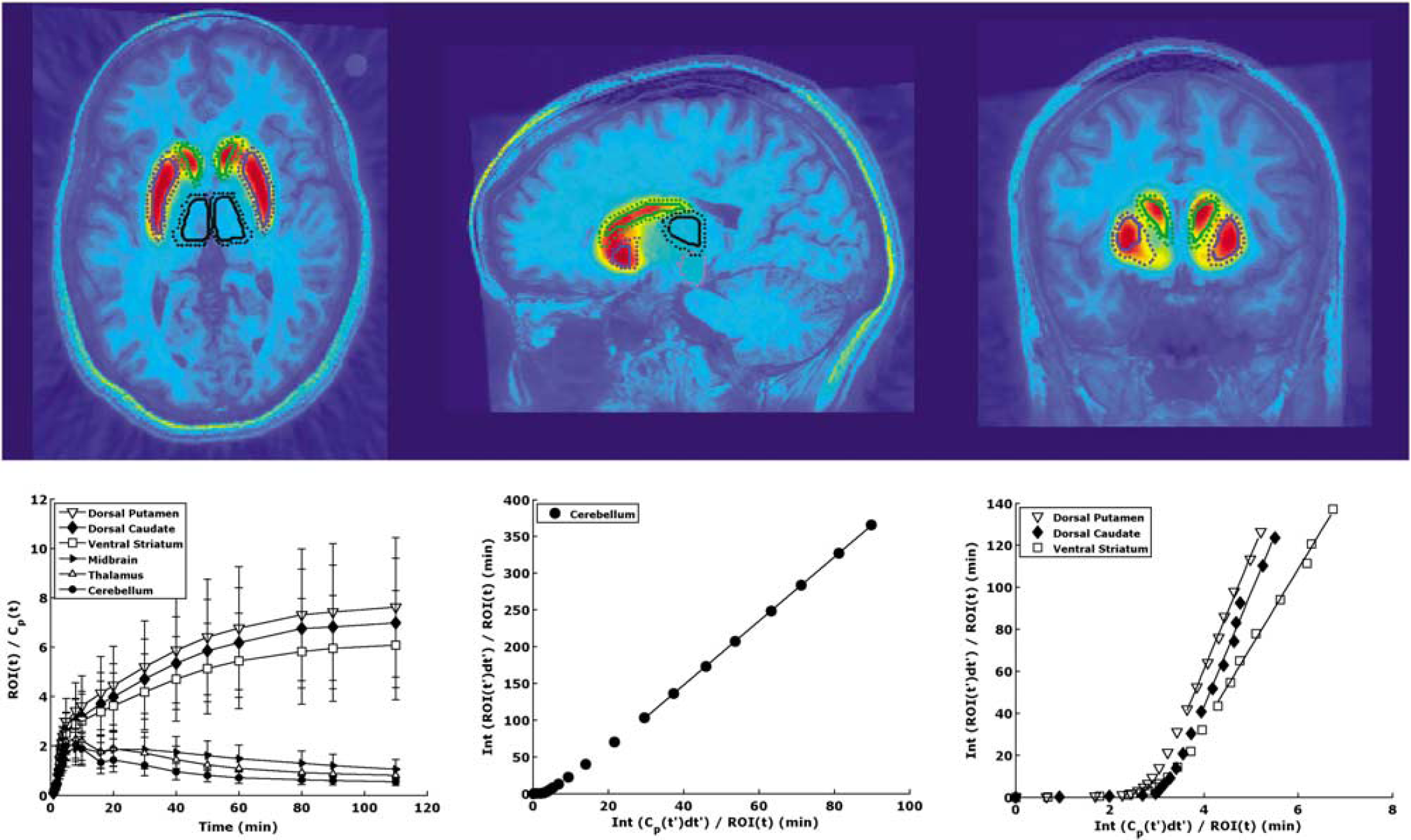
Top: PET images of [¹¹C]PE2l overlaid on MRI. These images show high accumulation of [¹¹C]PE2l in the striatal regions of the brain. For reference, outlines of ROIs based on automatic region of interest (ROI) delineation are shown. As the atlas is probabilistic, two outlines of each region are created. The dotted lines show the outline of the region with probability > 10% and the solid lines show the outline of the region with probability > 50%. The caudate, putamen, midbrain, and thalamus are shown (green, blue, magenta, and black outlines, respectively). Bottom: left: tissue-to-plasma ratios. High binding striatal subregions take longer to reach equilibrium than the lower binding midbrain, thalamus, and cerebellum. Middle and right: Logan plots for one subject. These plots were created using the Logan graphical analysis on the cerebellum (middle) or striatal subregions (right). A linear portion of the plot was achieved in all cases, as indicated by the fitted line.

Reference Region Determination

Most reference tissue methods rest on the assumption that binding kinetics in the reference region are adequately described by a 1TC model (Logan et al, 1996). In PE2I studies, the cerebellum has been used as a reference region because of its negligible amount of DAT (Madras et al, 1998; Hall et al, 1999; Jucaite et al, 2006). Owing to this, one would expect the cerebellum to be described by a 1TC model, in which the one compartment represents the free and nonspecifically bound ligand. However, experimentally, it has been found that binding kinetics in the cerebellum are best represented by a two-tissue compartment (2TC) model (Jucaite et al, 2006). This could be caused by the binding of a PE2I metabolite, as has been observed in the rat brain (Jucaite et al, 2006; Shetty et al, 2007; Hirvonen et al, 2008), PE2I kinetics (i.e., a slow transfer rate between free and nonspecifically bound ligand), or specific binding. Although initial reports based on autoradiography (Hall et al, 1999) and monkey displacement and pretreatment studies (Halldin et al, 2003) suggest there is little or no DAT in the cerebellum, it is possible that even a low DAT density in this region cannot be neglected. This has been observed before, in the case of [¹¹C]WAY-100635, which clearly shows specific binding in the cerebellum despite the low 5HT_1A receptor density in that region (6.26 fmol/mg) and the fact that [¹¹C]WAY-100635 specific binding only accounts for 48% of the cerebellar volume of distribution (Hall et al, 1997; Parsey et al, 2005).

Regardless of the origin of the second tissue compartment, it would be useful to know from a modeling (and anatomic) point of view whether a 1TC reference region exists for this ligand. To determine whether the cerebellum contains such a subregion, k-means clustering was used to separate TACs calculated at each voxel of the cerebellum into clusters with similar attributes (Späth, 1985). The rationale behind this is as follows: If ligand binding within the cerebellum is heterogeneous, then the average TAC for that region is actually a mixture of two or more dissimilar TACs. Using the k-means algorithm, groups (or clusters) of voxels with minimal intracluster variance are distinguished. If variance is based on the Euclidean distance between TACs, this method can be used to divide the cerebellum into clusters of voxels with similarly shaped TACs. In this way, it may be possible to identify a cluster of voxels with a mean TAC that is well fit by a 1TC model. Further analysis on the basis of the location of the voxels and the mean/s.d. of the voxels' TACs will help determine whether those voxels represent a meaningful cluster that can serve as a reference region.

For preliminary analysis, the cerebellum was divided into four clusters, as suggested by an automated routine designed to optimize the number of clusters. Each of the four clusters was fit using both a 1TC and a 2TC model. Using AIC (Akaike's information criterion) (Akaike, 1974) to select between competing models, it was found that all four of the cerebellum clusters were better described by a 2TC model than a 1TC model (average AIC ± s.d. over the four clusters was −36.01 ± 0.72/-34.12 ± 0.67 and −83.68 ± 3.31/-82.82 ± 3.16, for the iterative/noniterative 1TC and 2TC methods, respectively). However, the cerebellum can be subdivided in numerous ways, which may affect the resulting clusters. To account for this, the entire analysis was repeated on either the gray matter of the cerebellum only or the white matter only, with the number of clusters varying from 50 to 250 (data not shown). However, for all analyses, the resulting clusters were always better described (resulted in a lower AIC measure) by a 2TC model. For completeness, in addition to the cerebellum, several other regions with known low specific binding were analyzed by cluster analysis. The cuneus, cingulate gyrus, dorsal and lateral prefrontal cortex, fusiform gyrus, gyrus rectus, and uncus were divided into 10 clusters each using the k-means algorithm. However, these subdivisions also failed to show a region describable by a 1TC model.

Modeling

Modeling procedures considered were reported in Ogden et al (2007), and can be separated into two types—kinetic and graphical. As in Ogden et al (2007), 1TC and 2TC models were calculated, both iteratively and noniteratively. Using noniterative methods, the experimental data are matched to the most similar curve in a library of precalculated functions, rather than performing a nonlinear least squares iterative fit. Therefore, these approaches are faster and less computationally expensive.

Another modeling approach, basis pursuit (Gunn et al, 2002), also compares the experimental data with a library of functions; however, this library is composed of basis functions. The optimal basis function is then chosen by minimizing the model-data fit and the model complexity.

An iterative 2TC-constrained algorithm was also tested, in which the ratio of kinetic constants, K₁/k₂, for each ROI is constrained to the ratio of K₁ to k₂ in the reference region (Parsey et al, 2000).

Graphical methods were the second type of approach used. Using the Logan (Logan et al, 1996) graphical analysis, outcome measures can be calculated from the slope of the linear part of an integral plot. The linear portion of the graph for PE2I was considered to be the last eight points. To reduce the bias introduced by the Logan approach (Slifstein and Lamelle, 2000), likelihood estimation in graphical analysis (LEGA) was also used (Ogden, 2003).

In addition to these methods, three methods that do not require blood sampling were applied—the simplified reference tissue model (SRTM; Lammertsma and Hume, 1996) and the bloodless versions of LEGA and Logan methods.

Outcome Comparison Metrics

Six outcome metrics were used to assess the performance of each approach. These metrics, which are defined in Ogden et al (2007), are as follows:

(1) Percentage difference (PD), measuring the absolute difference between test and retest values on the same subject, divided by their average.

(2) Within subject mean sum of squares (WSMSS), which indicates the variance of an outcome measure based on repeated measurements on the same subject.

(3) Variance, the square of the s.d. of the value across subjects.

(4) Intraclass correlation coefficient (ICC), which determines how much variability is because of differences between subjects as opposed to within the same subject. This measure varies between −1 and 1.

(5) Identifiability (ID), measuring the stability of the estimation, based on taking bootstrap samples of TACs of each subject (Ogden and Tarpey, 2006). Lower identifiability indicates more stable data.

(6) Time stability, the effect of scan time on the measurement variability. All outcome measures were calculated using the maximum time (120 mins) and at earlier time points (by neglecting the later frames). A scan time that yields average outcome estimations within 5% of the outcome measurement calculated at 120 mins, with a s.d. <10%, is considered stable.

Simulation Studies

To further compare the models, a simulation was performed, in which differing levels of noise were added to ideal TACs by the following formula:

$$\text{SD}(t_i)=\text{SF}{\left(\frac{e^{\lambda t_i}C(t_i)}{\Delta t_i}\right)}^{0.5}$$

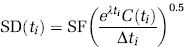
where SF is the scale factor, which sets the noise level, Λ the isotope decay constant, t _i the frame midtime, C(t _i ) the ideal activity at t _i , and Δt _i the frame duration (Logan et al, 2001). This technique provides a way to simulate the type of noise encountered in PET imaging, which increases as imaged radioactivity concentration increases and scan duration decreases. The simulations were performed on the dorsal caudate, dorsal putamen, ventral striatum, and cerebellum. A total of 1, 800 noisy TACs were generated for each ROI with the scale factor ranging from 0 to 2.7 for the high binding regions and from 0 to 1.8 for the cerebellum. Percentage added error was calculated as the mean PD between simulated noisy and ideal TACs. The 2TC iterative and noniterative, Logan, LEGA, and basis pursuit methods were applied to the noisy and ideal TACs, using an average input function and average injected dose from the 14 studies. Bias was calculated as the PD between outcome measures calculated from the ideal TAC and those calculated from the noisy TACs.

Results

Regional Uptake

[¹¹C]PE2I showed high accumulation in the striatal regions of the brain. (See Figure 1, top.) Although it is difficult to assess from the PET images, there is also an increased uptake in the midbrain and in the thalamus.

Tissue-to-plasma ratios were calculated by dividing the radioactivity within an ROI by the unmetabolized [¹¹C]PE2I concentration in the plasma at each time point. These results, shown in Figure 1 (bottom) indicate that tissue-to-plasma ratios take longer to peak in the high binding regions. By 30 mins, the tissue-to-plasma ratios were decreasing in the midbrain, thalamus, and cerebellum. In the dorsal striatum, the ratio was slightly increasing at the end of the acquisition time but the rate of increase had slowed.

Time Activity Curve Fits

To help clarify the differences between modeling methods, it is helpful to look at individual TACs (Figure 2). In particular, it is informative to examine TACs of the ventral striatum, a small region, which can be subject to image noise. As shown, the 2TC noniterative (2TCNI) and basis pursuit methods describe the data better than the other methods.

Figure 2

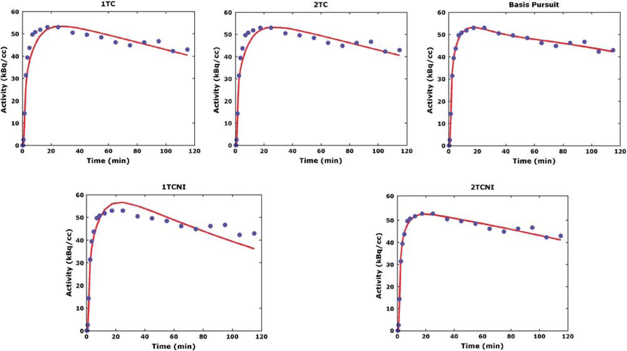
Time activity curves of one subject fit with five different methods. Only nongraphical methods using blood input are shown, indicating nontransformed data. The one-tissue compartment (1TC) methods (iterative and noniterative) do not describe most of the data, whereas the two-tissue compartment (2TC) methods (iterative and noniterative) describe the data well. Basis pursuit produces the closest fit to the data. 1TCNI, one-tissue compartment noniterative; 2TCNI, two-tissue compartment noniterative.

To determine whether this trend holds true for all subjects, the mean weighted sum of residuals for the nongraphical methods in the high binding regions (the manually outlined dorsal caudate, dorsal putamen, and ventral striatum) over all subjects was calculated. Basis pursuit produced the lowest mean residuals to the fit (0.04 ± 0.04). Application of the 1TC model, both iterative and noniterative, resulted in higher mean residual measurements (0.14 ± 0.18 and 0.30 ± 0.33, respectively), and the 2TC and 2TCNI methods performed similarly (0.10 ± 0.12 and 0.09 ± 0.10, respectively). The constrained 2TC model performed poorly. Therefore, it was excluded from subsequent analysis.

Outcome Measure Comparison

Although the outcome measure of interest is the receptor density, B_max, K_D (the equilibrium dissociation constant) cannot be determined simply. The outcome measure closest to the receptor density is BP_F (the ratio of the concentration of specifically bound ligand to free ligand in plasma at equilibrium, B_max/K_D); however, calculation of BP_F requires accurate measurement of the fraction of [¹¹C]PE2I not bound to plasma proteins, f_p. Owing to its low free fraction, f_p measurements of [¹¹C]PE2I are unreliable, making estimations of BP_F unreliable. Therefore, the measurement closest to receptor density, while maintaining reliability, is BP_P (the ratio of the concentration of specifically bound ligand to total ligand in plasma at equilibrium, BP_F × f_p). Thus, BP_P is used in this work for model comparisons, except when comparing reference region approaches.

Reproducibility studies were carried out to assess the extent of intraindividual variation (Figure 3, top left). The mean PD for the dorsal caudate, dorsal putamen, and ventral striatum varied from 9.2% to 15.6% across all methods and scan times. Except for two cases in which the iterative 1TC method attained a slightly lower PD, the 2TCNI method produced the lowest PD overall. In addition, the s.d. were lowest for the 2TCNI method at scan times >90 mins.

Figure 3

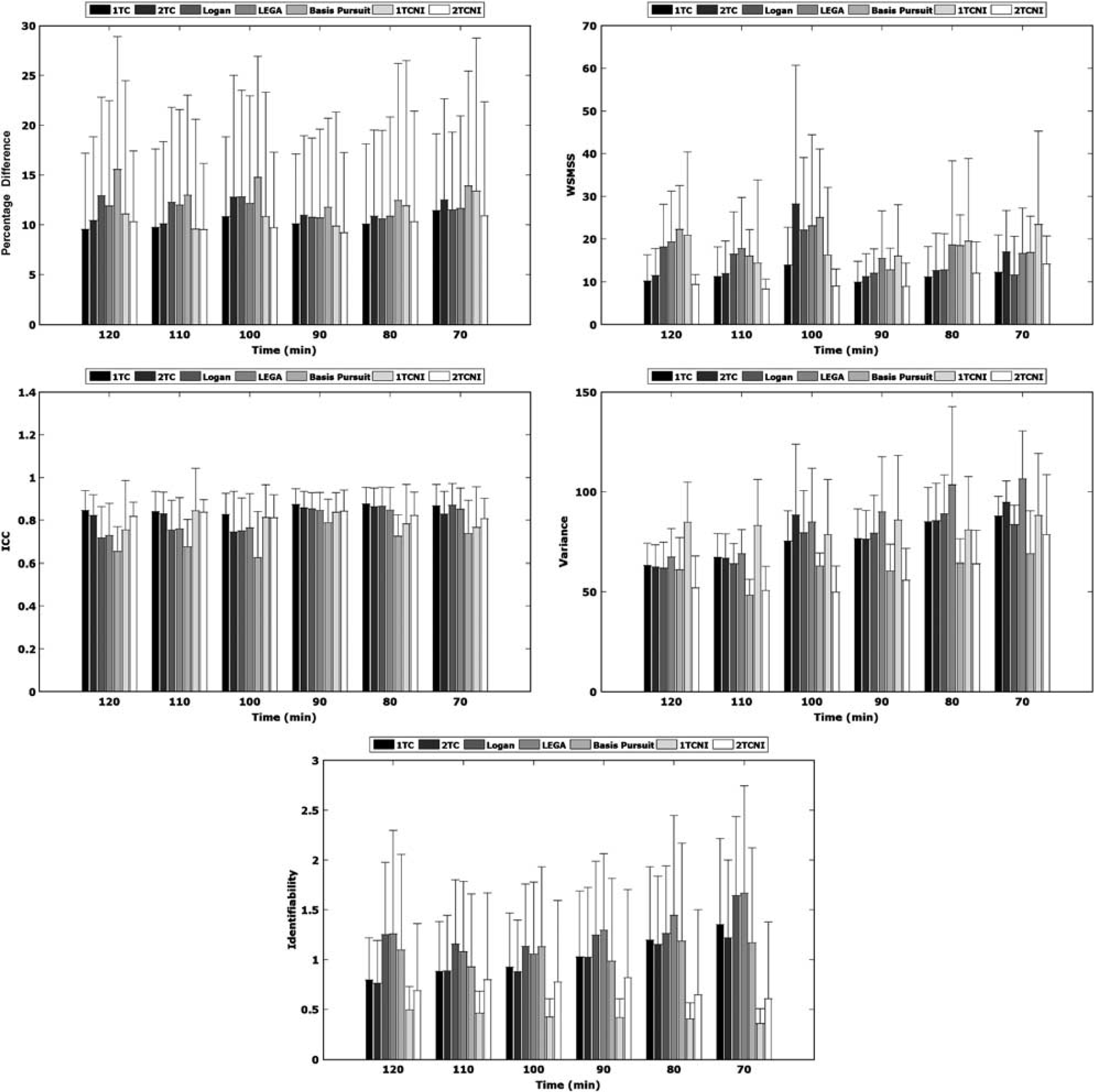
Mean percentage difference (top left), within subject mean sum of squared errors (top right), intraclass correlation coefficient (middle left), variance (middle right), and identifiability (bottom) on test–retest using seven methods. All metrics are based on BP_P Means were taken across all subjects in manually outlined high binding regions (dorsal caudate, dorsal putamen, and ventral striatum). Error bars indicate s.d. 1TC, one-tissue compartment; 2TC, two-tissue compartment; LEGA, likelihood estimation in graphical analysis; 1TCNI, one-tissue compartment noniterative; 2TCNI, two-tissue compartment noniterative

The WSMSS criterion is shown in Figure 3 (top right). At all scan times > 80 mins, the 2TCNI method performed the best; i.e., it produced the lowest WSMSS. Except for the 80 and 90-min scan times, 2TCNI also had the lowest s.d. of all the methods.

Reliability results are shown in Figure 3 (middle left). The ICC determines whether variance in the data resulted from intrasubject variability (low ICC) or between-subject variability (high ICC). The graphical methods yielded lower ICC values at the longer scan times. The basis pursuit method yielded significantly lower ICC than the other methods at all scan times. The 1TC and 2TCNI methods are the only methods that consistently produced ICC values > 0.8.

There is a trend of decreasing variance as the scan time increases (Figure 3, middle right). The 2TCNI and basis pursuit methods produced results with low variance, with the 2TCNI attaining the lowest variance at most scan times.

Results for identifiability (ID) are shown in Figure 3 (bottom). Although results for the Logan and LEGA methods are shown, these ID measures are based on only eight points (the linear points used for the measurement) and therefore, will be biased when shorter scan times (and therefore less points) are considered. Even with this bias, the range of ID values is small (0.36 to 1.67). The noniterative methods have an advantage over the iterative methods in that they produce lower ID values and are not as sensitive to scan time. The ID of the iterative methods improved as scan time increased, but always remained higher than the ID of their noniterative counterparts.

Table 1 shows the results of time stability analysis. Each number in the table is the minimum scan time required to reach a stable result as defined in the Materials and methods section. The 2TCNI method required the least amount of scanning time for a stable measurement and basis pursuit required the longest time, containing three cases in which a stable measurement did not occur before the maximum scan time (120 mins). Even with the 2TCNI method, 100 mins is required for a stable BP_ND measurement.

Table 1

Minimal scan times required for stable V_T, BP_P and BP_ND measurements

Models	2TC			Logan			LEGA			Basis			2TCNI
ROIs	VT	BPP	BPND	VT	BPP	BPND	VT	BPP	BPND	VT	BPP	BPND	VT	BPP	BPND
Dorsal caudate	80	80	100	90	100	110	90	90	100	90	90	110	70	70	100
Dorsal putamen	70	70	70	90	90	90	90	90	90	80	110	120	70	80	80
Ventral striatum	90	90	90	110	110	110	110	110	110	120	120	110	80	90	100
Mean	80	80	87	97	100	103	97	97	100	97	107	113	73	80	93
STD	10	10	15	12	10	12	12	12	10	21	15	6	6	10	12

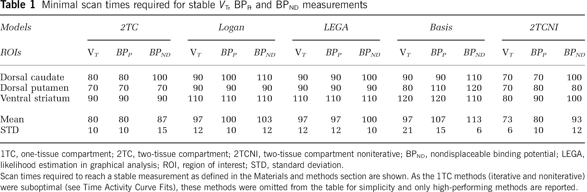
1TC, one-tissue compartment; 2TC, two-tissue compartment; 2TCNI, two-tissue compartment noniterative; BP_ND, nondisplaceable binding potential; LEGA, likelihood estimation in graphical analysis; ROI, region of interest; STD, standard deviation.

Scan times required to reach a stable measurement as defined in the Materials and methods section are shown. As the 1TC methods (iterative and noniterative) were suboptimal (see Time Activity Curve Fits), these methods were omitted from the table for simplicity and only high-performing methods are reported.

The results of this evaluation are summarized in Table 2, in which the top performing methods are ranked from one to four, on the basis of the six comparison metrics.

Table 2

Ranking of the four top methods

	2TC	Logan	LEGA	2TCNI
PD	2	4	3	1
WSMSS	2	3	4	1
ICC	1	3	3	2
Variance	2	3	4	1
ID	2	3	3	1
Time Stability	1	4	3	1

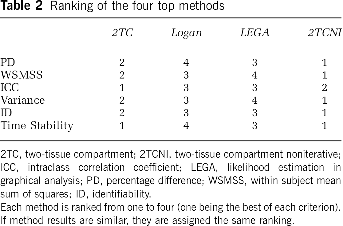
2TC, two-tissue compartment; 2TCNI, two-tissue compartment noniterative; ICC, intraclass correlation coefficient; LEGA, likelihood estimation in graphical analysis; PD, percentage difference; WSMSS, within subject mean sum of squares; ID, identifiability.

Each method is ranked from one to four (one being the best of each criterion). If method results are similar, they are assigned the same ranking.

Automated Regions of Interest

None of the outcome measures (V_T, BP_B and BP_ND) of high binding regions calculated using manually traced ROIs were statistically different, at a 5% significance level, from those calculated using automatically delineated ROIs. The slopes of the regression equation predicting outcome measures from manually segmented ROIs values by the automatically segmented ROI outcome measures were close to unity (1.01 to 1.33) with the intercept values ranging from −0.78 to −12.71, showing that outcome measures based on automated ROIs were similar but lower, in general, than those based on manual tracings. The outcome comparison metric results were also similar to those shown in Figure 3, although with slightly lower PD, WSMSS, and ID, as well as higher ICC and variance. See Table 3 for an example of this analysis using the 2TCNI at 100 mins.

Table 3

Metric results for automatically versus manually delineated ROIs usine 2TCNI at 100 mins

	Percentage difference	WSMSS	ICC	Variance	Identifiability
Auto ROIs	8.66 ± 7.19	6.72 ± 3.66	0.90 ± 0.06	63.49 ± 10.91	0.77 ± 0.44
Manual ROIs	9.72 ± 7.56	8.99 ± 4.04	0.81 ± 0.11	49.87 ± 13.02	0.78 ± 0.81

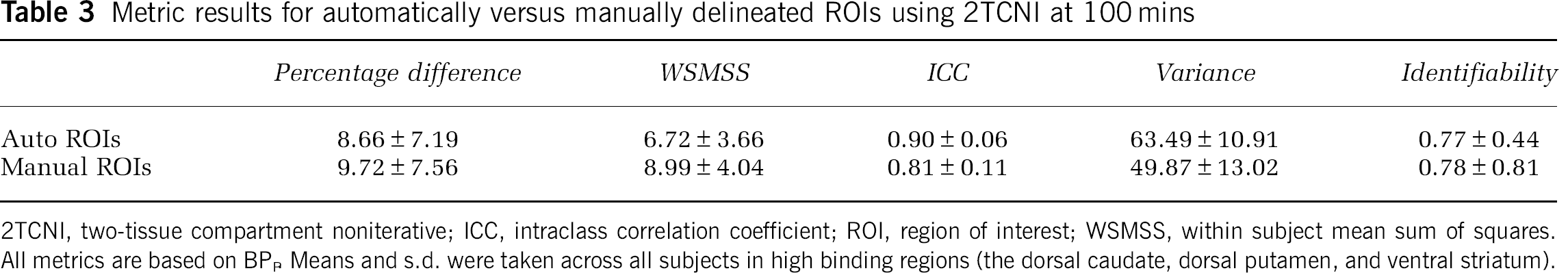
2TCNI, two-tissue compartment noniterative; ICC, intraclass correlation coefficient; ROI, region of interest; WSMSS, within subject mean sum of squares. All metrics are based on BP_P Means and s.d. were taken across all subjects in high binding regions (the dorsal caudate, dorsal putamen, and ventral striatum).

Simulation Results

Simulation results for the ventral striatum are shown in Figure 4. At low noise levels (> 5% to 10%), all of the modeling methods performed similarly. As added noise increases, the 2TCNI method produces less biased estimates than the other models. In addition, at high added noise levels (>15%), results produced by other models were erratic, whereas the bias of the 2TCNI method never increased above 16.9%. In addition, for every level of noise shown, the 2TCNI method resulted in a lower s.d. of the bias than the other methods. The results shown are similar to simulation results obtained using BP_P and are representative of the other ROIs examined. (Performing the same simulation using the dorsal caudate, dorsal putamen, or cerebellum, the maximum bias found using 2TCNI was 13.3%, 14.7%, and 12.9%, respectively, whereas the maximum bias produced by the iterative 2TC method was significantly higher than 50% in all regions.) In the case of the cerebellum, the graphical approaches produced the lowest bias estimates when large amounts of noise were added; however, the 2TCNI method still performed better than the iterative 2TC approach.

Figure 4

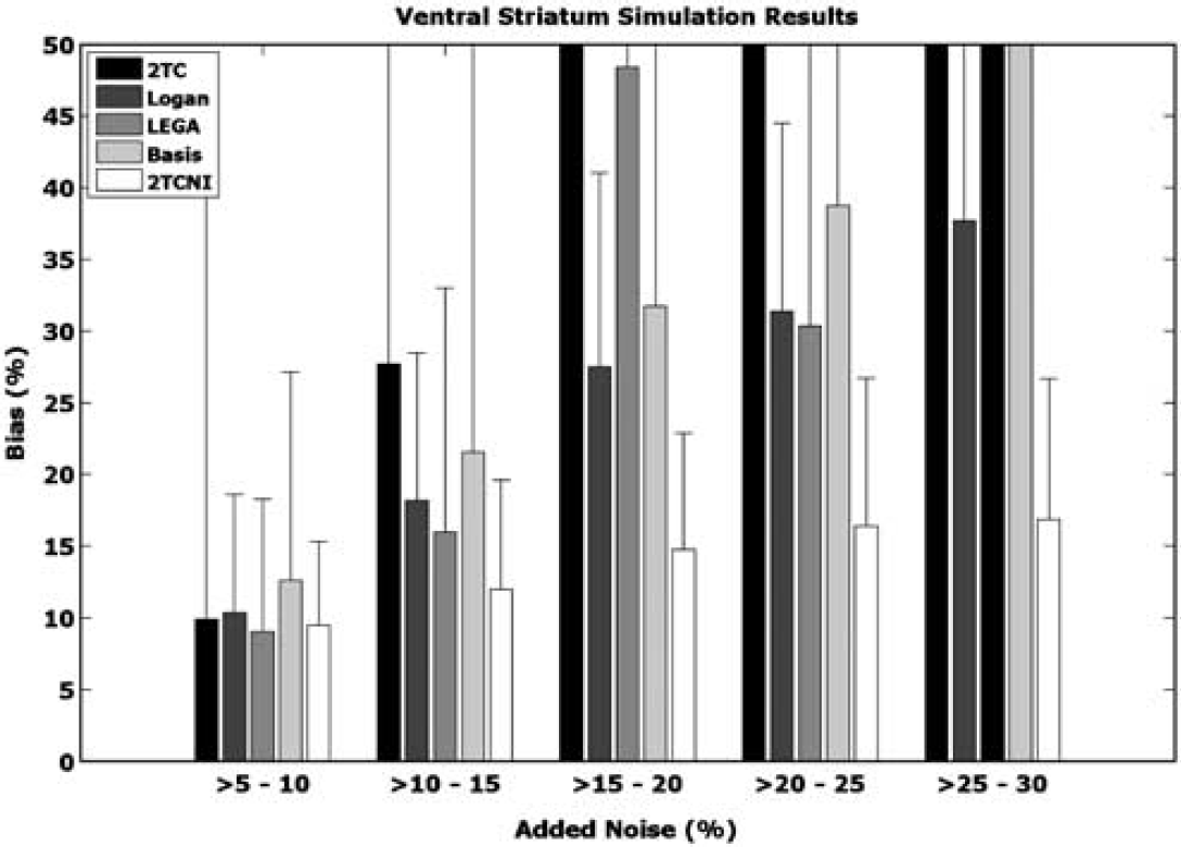
Simulation results. Various amounts of noise were added to ideal time activity curves (TACs) of the ventral striatum. The bias between the volume of distribution (V_T) obtained from the noisy TACs and V_T based on the ideal TAC was calculated and plotted. At least 200 noisy simulations were performed in each noise range, from which s.d. was calculated. The maximum bias displayed is 50%, although some methods yielded higher biases. 2TC, two-tissue compartment; LEGA, likelihood estimation in graphical analysis; 2TCNI, two-tissue compartment noniterative

Two-Tissue Compartment Noniterative Results

The outcome measure comparisons performed in this paper were based on aggregate measures of the highest binding regions (the dorsal caudate, dorsal putamen, and ventral striatum). As an atlas was used to delineate a greater number of ROIs, metrics can also be calculated for each of those ROIs. The results of that analysis, for every ROI with a BP_P >0.5, is shown in Table 4.

Table 4

ROI metric comparison

	Mean BPP	PD	WSMSS	ICC	Variance	ID
Dorsal putamen	39.30 (42.62)	11.46 (7.08)	11.77 (4.81)	0.86 (0.92)	76.24 (54.04)	0.81 (0.81)
Dorsal caudate	37.58 (39.41)	7.61 (8.43)	6.39 (7.89)	0.91 (0.80)	62.72 (37.32)	0.60 (0.74)
Ventral striatum	29.81 (31.74)	10.15 (11.76)	9.00 (11.56)	0.84 (0.74)	52.94 (41.54)	0.96 (0.78)
Midbrain	2.32	12.37	0.04	0.90	0.35	0.06
Insula	2.00	16.17	0.05	0.94	0.83	0.09
Thalamus	1.45	14.83	0.06	0.86	0.38	0.05
Amygdala	1.37	51.31	0.41	0.39	0.65	0.19
Brainstem	0.95	16.99	0.02	0.75	0.09	0.05
Hippocampus	0.81	28.12	0.04	0.80	0.18	0.06

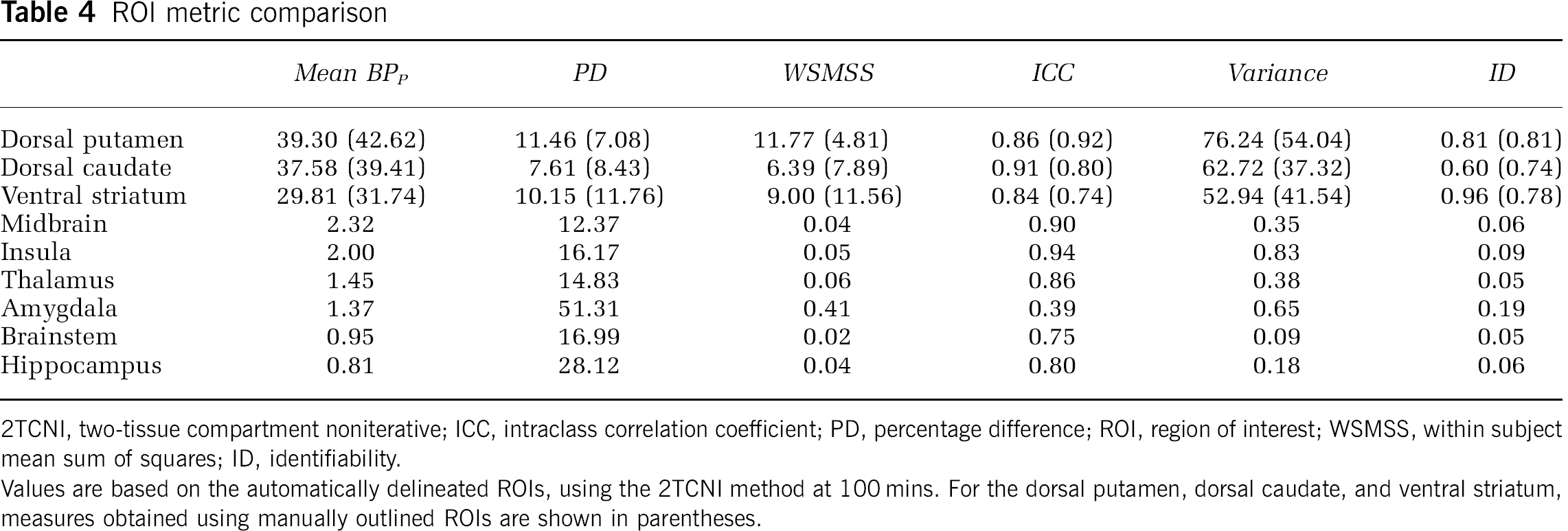
2TCNI, two-tissue compartment noniterative; ICC, intraclass correlation coefficient; PD, percentage difference; ROI, region of interest; WSMSS, within subject mean sum of squares; ID, identifiability.

Values are based on the automatically delineated ROIs, using the 2TCNI method at 100 mins. For the dorsal putamen, dorsal caudate, and ventral striatum, measures obtained using manually outlined ROIs are shown in parentheses.

Reference Region Approaches

Comparison of outcome measures can also be performed using reference region approaches, although these numbers should not be compared directly with methods using arterial blood information because assumptions about binding kinetics in the cerebellum can result in lower values for each outcome measure, skewing the estimates. Performing this analysis (without identifiability, which is unavailable for reference region approaches) showed that bloodless LEGA and Logan performed significantly better than the SRTM method (28.8% lower PD, 73.8% lower WSMSS, and 50.1% lower variance on average, as well as 25.5% higher ICC on average). Although the results from Logan and LEGA were similar, use of the Logan method resulted in a slightly lower mean PD (3.3%), lower variance (27.1%), and WSMSS (15.7%), with a slightly higher ICC (2.8%) than LEGA at most scan times.

In addition, BP_ND values determined using the bloodless Logan and LEGA had a higher correlation than SRTM did to BP_ND values calculated by 2TCNI (correlation coefficient of 0.99 for Logan and LEGA versus 0.96 for SRTM). When BP_ND values calculated using reference tissue approaches were plotted versus BP_ND values calculated using the 2TCNI method, the slope of the regression line was similar for Logan and LEGA (0.56 and 0.58, respectively), as was the sum of the residuals (6.84 and 7.01, respectively). Using SRTM, the slope was higher (0.69) but the residuals were also higher (16.22), although SRTM estimates more parameters than Logan or LEGA.

Voxel Level Analysis

The results presented thus far have been based on ROI analysis and rely on mean estimates of activity within an ROI. Such analysis can also be performed on a voxel level. In this case, the outcome measures are determined at each voxel.

To determine whether voxel-based methods can produce accurate outcome metric estimates, V_T measurements of the high binding regions calculated using 2TCNI on an ROI-level were compared with those averaged within an ROI from a 2TCNI V_T voxel image. The slope of the regression line comparing ROI with voxel estimates was close to unity (0.95) with an intercept of 1.32.

Discussion

The primary objective of this work was to determine the optimal modeling technique for [¹¹C]PE2I in humans. This was accomplished by assessing 11 possible modeling methods using six metrics on the outcome measure BP_P (or BP_ND for reference region approaches). The analysis was performed with automatically and manually delineated ROIs, using blood input functions or a reference region, both on an ROI and voxel level, and with simulation studies.

Without reliable image processing procedures, poor metric performance can result, regardless of the applied model. Owing to this, all PET-to-MRI coregistrations performed in this study were based on a parameter optimization technique, which has been developed earlier and validated in this lab.

Regional Uptake

The results of brain uptake analysis are consistent with those of earlier studies. Highest uptake was observed in the caudate and putamen, followed by the ventral striatum, midbrain, thalamus, and cerebellum (Jucaite et al, 2006; Leroy et al, 2007; Hirvonen et al, 2008; Ito et al, 2008). The binding outside the striatal regions was low.

Modeling Method Assessment

Modeling techniques were compared on the basis of the assessment of model fit and six different metrics. Both compartment models and graphical approaches were assessed. This was possible because of the length of scan time, which resulted in the linear portion of the integral plots being reached (Figure 1).

Initial assessment of a 2TC-constrained model showed that it performed poorly, both in fitting the data and in comparing outcome measures. This may be because of the existence of a second compartment in the reference region, which could affect the calculations of K₁ and k₂ in this region. The resulting error would then be propagated through each ROI outcome measure calculation owing to the constraint.

Although the comparison metrics determine the repeatability of a model, each model's accuracy depends on its fit to the data. Therefore, when evaluating potential models, it is important to consider not only their performance based on metrics, but also, how well they fit the raw experimental data. The iterative 1TC and 2TC models performed comparably with regard to the comparison metrics, with relatively low PD, WSMSS, and variances, as well as with relatively high ICC. However, between the two models, the 2TC model is better able to fit the TAC of each ROI because it has more degrees of freedom (Figure 2). The extra parameters (kinetic constants k₃ and k₄) of the 2TC model are required to fit the TACs because of the second (specific binding) compartment in these ROIs. The time required to reach a stable measurement using a 2TC is also reasonable (Table 1).

The basis pursuit method has the most degrees of freedom because of the number of basis functions used in curve fitting, allowing this method to fit the data the best (in terms of minimizing the model-data residuals). However, this happens at the expense of overfitting. As a result, any amount of noise can drastically change the model fit, resulting in unreliable results. Because of this effect, basis pursuit does not perform well on the basis of comparison metrics and also requires the longest scanning time of any method to reach stable results.

The Logan and LEGA methods performed similarly. The LEGA method produced higher ICC values than Logan at longer time points, with the reverse being true at shorter time points. Moreover, LEGA yielded a slightly lower PD, whereas Logan had lower WSMSS and variance, in general. This could be a result of the fact that, because of the reduction in bias, LEGA values are, on average, higher than those determined using Logan. (The Logan values may have lower variances and WSMSS simply because the values are lower.) None of the two methods performed as well as the compartment models, in general. In addition, both methods required more scanning time to achieve stable results than either the 2TC or 2TCNI methods.

The 1TCNI (1TC noniterative) method performed worse than the iterative 1TC method for the six metrics at almost every time point. In addition, the 1TCNI method has the highest mean residual error, because of the combination of the small number of parameters being fit (same as the 1TC model) and being limited to a predefined set of function possibilities (because it is noniterative). The result is a method that is neither accurate nor repeatable.

The 2TCNI method, in contrast, performs best in most metrics, with the exception of ICC. The PD measures are lowest of any method at most time points and variance/WSMSS values are markedly low. The ICC values determined using 2TCNI are comparable with the other compartment models, although slightly lower. Owing to the complexity of noisy image data, iterative methods can become trapped in a local minimum while trying to fit the later TAC points and may not adequately capture the TAC peak. (See Figure 2.) As the 2TCNI method does not iteratively optimize the solution, it is less sensitive to initialization and can fit noisy data well. This was confirmed by the simulation experiments, which showed that the 2TCNI method not only reduced the bias of outcome measure estimates on noisy data, but also produced estimates that had lower variance than those produced by other methods.

The time required for the 2TCNI method to reach a stable measurement is comparable with that of the iterative 2TC method, and less than the Logan or LEGA methods. In addition, the 2TCNI method has the added advantage that it is faster and less computationally intensive than the iterative methods (making voxel analysis more feasible).

Previous authors have found that the 2TC model fits the data best (Jucaite et al, 2006; Hirvonen et al, 2008). This is consistent with the current analysis, showing that the 2TC model performs well in all metric categories. However, previous authors have not attempted to fit the data using a 2TCNI method, which has been shown to be the top performer here.

Automated Regions of Interest

Results obtained using automatically delineated ROIs were similar to those found using manually outlined ROIs. In general, outcome measurements determined using automatic ROIs were lower (although not significantly) than their manually outlined counterparts. (See Table 4, for example.) The ICC values were generally higher for the automated ROIs; however, so were the variances. These findings can be explained by the fact that automatically drawn ROIs are usually larger than those drawn manually (because the registration that brings the atlas into the space of the subject's MRI will not always perfectly capture the outline of each ROI). As [¹¹C]PE2I binding mostly occurs in the striatum, if a striatal ROI is drawn too large, it will inevitably contain some of the adjacent lower binding regions. This will lower the overall estimate of that region's binding and dramatically increase the variance. As the automatically drawn regions are larger, however, they can be less prone to the effects of noise, which can serve to increase the reliability (increase ICC values) and stability (decrease ID values).

Although it is important to note the differences between automatically and manually generated ROIs, the similarities are such that automatically generated ROIs can approximate those drawn manually, depending on the application, and can be used to provide a quick first look at the outcome measures.

Two-Tissue Compartment Noniterative Results

The BP_P values determined using the 2TCNI method were highly correlated with those estimated by the iterative 2TC method (correlation coefficient = 0.99) and the values were similar (slope and intercept of the regression line predicting 2TCNI BP_P values from 2TC BP_P values were 0.99 and 0.27, respectively). Therefore, these 2TCNI values can be directly compared with results obtained from the 2TC method. The values of the outcome measures (using both manual and automated ROIs) found in this study were similar to those of earlier reports in which an HR+ scanner was used (Jucaite et al, 2006; Leroy et al, 2007; Ito et al, 2008).

The most comprehensive modeling work using PE2I to date was performed by Hirvonen et al (2008). In that study, a high resolution PET scanner was used, which has been shown to yield up to 35% higher binding potential estimates in high binding striatal regions (Leroy et al, 2007). Comparing the high binding dorsal caudate, dorsal putamen, and ventral striatum, mean BP_ND values as determined by the 2TCNI at 70 mins (10.53 ± 1.53, 11.30 ± 2.46, and 9.11 ± 1.68, respectively) were on average ~75% higher in Hirvonen et al (2008). This could be because of differences in the nondisplaceable volume of distribution measurement, which affects BP_ND (and can be compounded by scanner differences). However, BP_P and V_T values at 70 mins were not as disparate for these three regions (values in Hirvonen et al (2008) are 40% to 46% higher, on average, for BP_P and V_T). At 70 mins, 2TCNI yielded a BP_P of 39.67 ± 6.98, 42.79 ± 10.63, and 34.60 ± 7.88 for the dorsal caudate, dorsal putamen, and ventral striatum, respectively.

Reference Region Methods

As plasma analysis requires invasive blood sampling and is time-intensive, it would be advantageous if a modeling technique that performed as well with blood input as it did without such an input was used. Three possibilities were examined in this paper, namely the bloodless versions of Logan and LEGA, and SRTM. In terms of outcome metrics, bloodless Logan and LEGA performed similarly. However, the Logan method performed slightly better (lower PD, WSMSS, and variance, with higher ICC at most time points). Both methods performed better than SRTM, which attained the lowest ranking in every metric comparison.

When the outcome measures calculated by reference region approaches were plotted against the same measure calculated using the top performing 2TCNI method, the values of the slopes were consistent with earlier published reports, which showed that the reference region methods resulted in BP_ND values that were approximately half of those determined using plasma data (Hirvonen et al, 2008). This is most likely because of the violation of the 1TC kinetics in the cerebellum (Hirvonen et al, 2008).

Simulation studies have shown that violating the 1TC assumption of SRTM leads to an underestimation of BP_ND, which increases with increasing values of BP_ND (Slifstein et al, 2000) and, as expected, BP_ND estimates in the high binding striatum are markedly low using SRTM. It has also been shown that BP_ND is underestimated using the Logan approach in the presence of noise (Slifstein and Laruelle, 2000). However, LEGA has been specifically designed to decrease this bias (Ogden, 2003). Therefore, the fact that both the Logan and LEGA methods yielded lower BP_ND values, may indicate that some specific binding occurs in the cerebellum, increasing the concentration of the ligand in the reference region, and therefore decreasing the overall BP_ND estimate. However, as indicated by the high correlation between 2TCNI and reference region results, this bias does not preclude reliable analysis using reference region approaches.

PE2I Metabolites

As discussed above and as reported previously, PE2I metabolite binding occurs in the brain and may affect outcome measure calculations (Jucaite et al, 2006; Shetty et al, 2007; Hirvonen et al, 2008). Between two and three radioactive metabolites have been identified in human studies (Jucaite et al, 2006; Hirvonen et al, 2008). In addition, rat studies have shown that, 30 mins after injection, unmetabolized [¹¹C]PE2I accounts for 92.5% of the total radioactivity in the striatum, but only 67.1% of the total radioactivity in the cerebellum (Shetty et al, 2007). As a possible consequence, if the metabolism rate is affected (which may occur, e.g., during treatment studies), this ligand may yield unreliable results. However, as shown in this work, PE2I metabolite binding does not seem to adversely affect test–retest reliability, indicating the feasibility of PE2I use for certain applications.

Voxel-Based Analysis

It is important for a voxel-based method to agree with the best ROI-based method. In this work, the values of outcome measures calculated using the 2TCNI method on a voxel level correlated very highly with those determined on the ROI level. This means that the 2TCNI voxel analysis is reliable and can be used to increase the understanding of ligand binding, because of the increased spatial information provided by voxel modeling.

Conclusions

In this study, 11 different modeling techniques were tested using 6 outcome measures. Of the three reference region methods tested, the Logan and LEGA methods produced similar results and performed better than SRTM. However, all reference region methods resulted in lower values of BP_ND than when blood input was used. This could be because of the second compartment in the reference region. Although clustering techniques were extensively applied to various brain regions in search of a reference region that did not violate the 1TC assumption, it does not seem that [¹¹C]PE2I produces such a region. Therefore, this will remain a problem for reference region approaches.

When plasma analysis is used, it was found that the 2TCNI method with at least 100 mins of scan time is optimal. This method not only fit the data well, but also was the top-ranked method for almost all metrics. It was also shown to be the most robust method tested in simulation studies.