Statistics in Experimental Cerebrovascular Research—Comparison of Two Groups with a Continuous Outcome Variable

Abstract

Part one of this mini-series on statistics in cerebrovascular research uses the simplest yet most common comparison in experimental research (two groups with a continuous outcome variable) to introduce the very basic concepts of statistical testing: a priori formulation of hypotheses and definition of planned statistical analysis, error considerations, and power analysis.

Experimental Design

For ethical and economic reasons, it is important to design animal experiments properly, analyze the data correctly, and to use the minimum number of animals necessary to achieve the scientific objectives of the study (Festing and Altman, 2002). Recently, evidence has been presented that weaknesses in design, analysis, and reporting in experimental stroke research are prevalent (Dirnagl, 2006), and that these weaknesses can have quantifiable effects on the predictiveness and ultimately on the validity of preclinical research in the cerebrovascular field (Crossley et al, 2008; Macleod et al, 2008). A systematic analysis of all papers reporting original research and published in the Journal of Cerebral Blood Flow and Metabolism in 2008 has revealed that deficiencies in experimental design, statistical analysis, and reporting of data are very common (Deister, Schlattmann, Dirnagl, unpublished). In a concerted action, a series of measures to reduce bias in the design, conduct, analysis, and reporting of animal experiments modeling human stroke has been proposed and published simultaneously in several journals in the field including the Journal of Cerebral Blood Flow and Metabolism (Macleod et al, 2009).

We would like to guide researchers of this journal with a mini-series on the design of experiments, as well as the analysis, interpretation, and presentation of data. In the first article, we will start with the comparison of two experimental conditions, which is one of the most frequent trial designs in stroke research. This simple design allows us to introduce the very basic concepts of Null Hypothesis statistical testing: a priori formulation of hypotheses and definition of planned statistical analysis, error considerations, and power analysis, as well as proper reporting of the data. In future articles, we will progress to multiple comparisons as well as the analysis of categorical variables (such as most scores in outcome evaluation).

Where ever possible, to minimize bias in biomedical research, experiments require randomized allocation to experimental groups and outcome assessment without knowledge of the assignment to these groups. We start by formulating a hypothesis (e.g., ‘Compound X is a neuroprotectant and affects injury after focal cerebral ischemia’), and then choose an appropriate study design. After we have selected an adequate outcome measure, the sample size of the study needs to be determined a priori. The primary outcome measure in experimental stroke research is very often a change in infarct volume caused by an intervention (pharmacological, genetic, etc.), but it could be a change in behavior, or cerebral perfusion, among many other possibilities. It is noted that in this stage of planning, inclusion and exclusion criteria need to be set, and provisions for randomized allocation and blinding (experimental manipulations, outcome assessment) need to be made. The principal workflow of planning and conducting such a study in its most abstract form is shown on the left panel of Figure 1, whereas a corresponding example is given on the right.

Figure 1

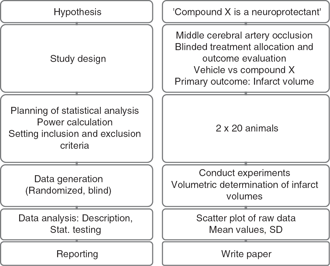
Study workflow (left panel: principle; right panel: corresponding example).

Errors and Sample Size Calculation

The sample size of the study depends on the error we are prepared to live with. This error is of two types. The type I error is the probability of false-positive results or, in other words, declaring a treatment difference where none exists. This is also known as significance level or α-level and is usually fixed not by reasoning but purely by convention at α = 5% (two-sided).

But what does it mean if we find that our results are significant on the 5% level? Please consult Table 1 and see which interpretations you agree with!

Table 1

Interpreting α-level and P-value. Which one of the following statements is correct? (after Mulaik et al, 1997)

1.	The P-value of a significant test is the probability that the research results are due to chance
2.	A hypothesis accepted as significant at the α-level of significance has the probability of 1–α of being found significant in future replications of the experiment
3.	A hypothesis accepted as significant at the α-level of significance has a probability of 1–α of being true
4.	The size of P of the significance level of a result is an index of the importance or size of a difference or relation
5.	The probability of rejecting H0 is α

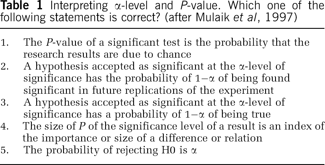
Some researchers will pick at least one of the choices of Table 1. However, none of those interpretations is correct! What an α-level of 5% really implies is that if we were to repeat the analysis many times, using new data each time, and if the null hypothesis (H0) were really true, then on only 5% of these occasions would we (falsely) reject it.

H0 usually states the opposite of what we really want to find, namely that there is no difference between the two groups. As we are performing the statistical test under the assumption that H0 is true, it is impossible that we make a probability statement about H0 at the same time. We cannot assess what we assume to be true (Goodman, 1999)! Thus, P-values cannot be error probabilities, that is tell us whether our results are due to chance. In addition, as given a high enough n even with minor group differences, we will be able to reject any H0, no matter what the setting is, α or P can also yield no index of biological significance; they make our results ‘sizeless.’ In other words, rejecting H0 is a trivial exercise because stating that two treatments or samples are identical ( = H0) is always false, and rejecting it is merely a matter of carrying out enough experiments (i.e., having enough power, see below, and Kirk, 1996).

The type II error is the false-negative rate or probability of failing to detect a treatment difference that actually exists. It is also called the β- error and 1–β is known as the power of the study. Power is the conditional probability of accepting the alternative hypothesis (H1, that there is a difference) when it is true. Regulatory agencies like α (consumer risk) to be low. Researchers like β (producer risk) to be low. Power increases ( = β decreases) with effect size (e.g., reduction in infarct size): the larger the difference between the parameters tested, the greater the power to detect it. Increasing sample size decreases the standard error, thereby also increasing power. Conversely, a large variance (i.e., s.d.) will decrease power. Note that there is an inverse relation between α and β: increasing α increases power ( = decreases β), but also increases the risk of rejecting H0 when it is actually true.

Let us fix α at 5% and β at 20%, a value often chosen. Researchers seem to be more afraid of a false-positive than a false-negative result. To plan the study, we make the assumption that our data follow a normal distribution with common s.d. σ and means μ₁ and μ₂. The difference of means δ = μ₁–μ₂ is often called the effect size. The ratio of difference and common s.d.

$\mathrm{\Delta }=\frac{\delta }{\sigma }$

is called the standardized effect. For example, a reduction of infarct size by δ = 30 mm³ results in a standardized effect size Δ = 1 if σ was also 30 mm³. These definitions of effect size may be found in the book by Hulley et al (2007).

Sample size estimation for two independent samples requires several assumptions and specifications. A minimally relevant effect difference δ and the common s.d. need to be ‘guesstimated’. To ‘guesstimate’ δ, we need previous experience with the model; setting d is a matter of pathophysiological reasoning. In addition, the significance level a and the desired power need to be set.

If we, for example, want to be able to detect a reduction in the infarct volume of at least δ = 15 mm³ (effect size), and we expect a s.d. of σ = 30 mm³, at 80% power and α = 0.05 (two-sided) we need a total sample size of 128 animals, that is 64 per group based on the two sample t-test. All major statistical packages calculate sample size (or power, given the sample size). If you do not have access to these commercial programs, a simple, free program is available on the internet (Faul et al, 2007). Alternatively, web browser-based routines allow you to calculate power and sample size directly on the internet (e.g., SISA, url see references).

A simple rule of thumb (van Belle, 2008) can also be used to estimate sample sizes for a two-sided α = 0.05 and 80% power:

$n=\frac{16}{{\mathrm{\Delta }}^2}$

If we set standardized effect size Δ to 0.5, that is, we want to be able to detect a difference of half the s.d., then 16/0.5² = 64 subjects per group are needed.

Similar to the type I error, the concept of type II error is often misunderstood, and consequently power and sample size calculation have no role in the overwhelming majority of papers in the cerebrovascular and experimental stroke field. Quiz yourself and try to evaluate the statements in Table 2.

Table 2

Interpreting power and type II error. Which one of the following statements is correct?

1.	Power calculations are only necessary if a negative result (i.e., no significant P-value) was obtained
2.	Power should be calculated after the experiment, since only then do we know the effect size
3.	If P < 0.001, β is not of practical relevance
4.	Power and sample size calculations are relevant in clinical trials or translational preclinical research, but not in explorative basic research

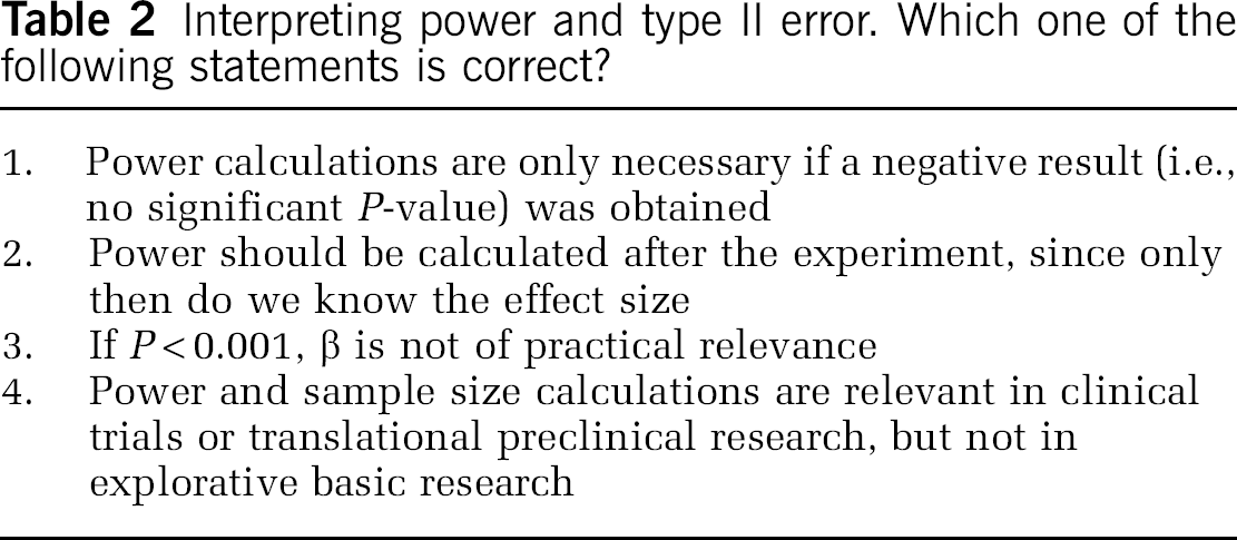
As in Table 1, none of the statements in Table 2 is correct! The prototypical misunderstanding of the type II error is that if one has obtained a statistically significant P-value (e.g., P < 0.05), there is no need to waste time worrying about type II errors a priori. Didn't we reject H0? For various reasons, this is a fallacy with potentially calamitous impact. When H0 is in fact false (the drug really works, the knockout mouse has a phenotype, etc.), the overall error rate is not the α level, but the type II error rate β (Schmidt and Hunter, 1997). It is impossible to falsely conclude that H0 is false when in fact it is false! This trivial insight may have important consequences for the interpretation of experimental data in cerebrovascular research and ultimately for its translation to text book or patient: If β is high (i.e., statistical power is low), the probability of being able to reproduce data decreases more and more. For example, at a power of 0.5, which is not uncommon in present cerebrovascular research (Dirnagl, 2006), the probability of being able to replicate the findings of a study stands at 50% (Mulaik et al, 1997)!

Descriptive Statistics

Categorical data such as behavioral scores or presence or absence of symptoms can be summarized as frequencies and percentages. Continuous data such as infarct volume may be summarized using the mean and s.d. Table 3 shows data from a typical experimental stroke experiment and corresponding summary statistics.

Table 3

Infarct volumes of a mouse stroke experiment

	Group 1	Group 2
	167	88
	198	99
	140	113
	166	117
	141	103
	92	135
	76	100
	126	116
	157	90
	114	100
	160	76
	118	108
	120	104
	160	63
	124	85
	146	78
	98	92
	127	101
Mean	135.0	98.2
s.d.	30.5	17.0

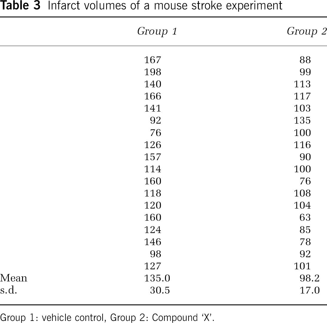
Group 1: vehicle control, Group 2: Compound ‘X’.

For descriptive purposes, only the s.d. of the data is an acceptable measure, but not the standard error of the mean (s.e.m.). The latter is an estimate for the precision of estimating the mean, not a description of the sample (Altman and Bland, 2005).

Graphical Display of the Data

It is very common in cerebrovascular research, but unsatisfactory, to summarize the results of a two-group comparison of continuous variables with a bar graph and s.e.m.s. s.e.m.s should not be used for graphical data presentation (or for data presentation in the text, see above). Second, displaying only the mean is the least informative option available. A very useful graph is the box-and-whisker plot, which is helpful in interpreting the distribution of data (see Figure 2). A box-and-whisker plot provides a graphical summary of a set of data based on the quartiles of that data set: quartiles are used to split the data into four groups, each containing 25% of the measurements. By combining the box-and-whisker plot with a display of each data point as a scatter plot, a most informative data display can be obtained.

Figure 2

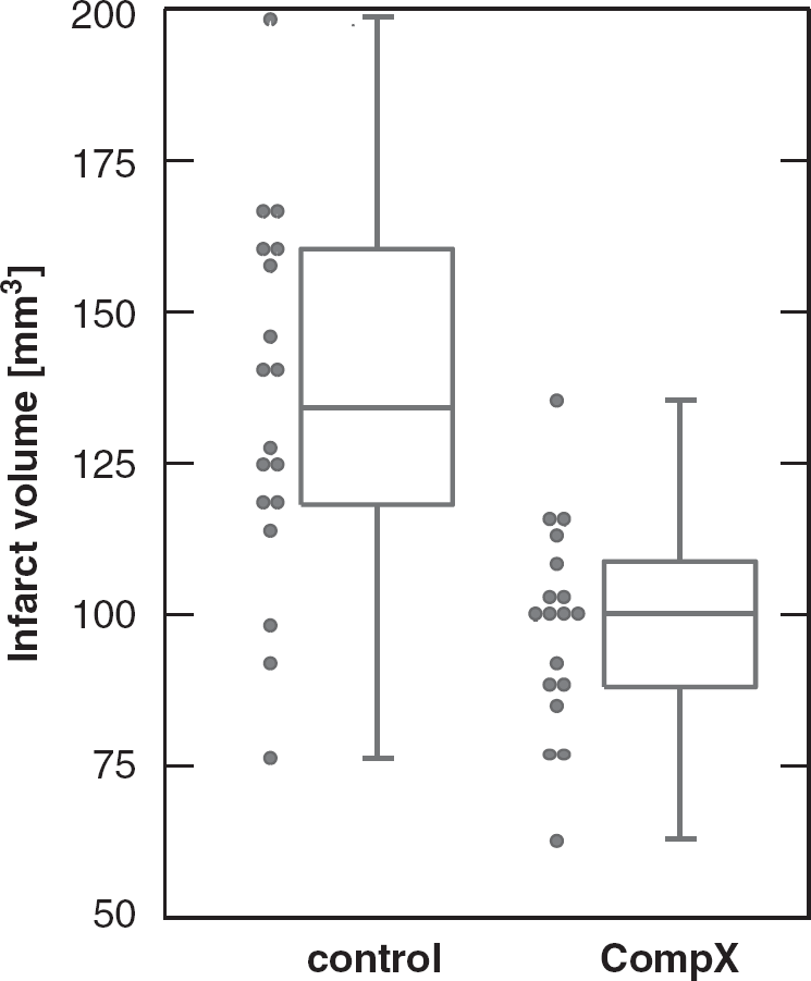
Box-and-whisker plot (median, first and third percentiles, range) of the infarct volume data of Table 3, displayed with the scatter plot of raw data.

Confirmatory data analysis

A properly designed experiment in which the hypotheses are stated and type I and II error considerations as well as the plan for statistical analysis are specified in advance—and ideally published later—allows a confirmatory analysis. In such experiments, the key hypothesis of interest follows directly from the experiment's primary objective, which is always predefined, and is the hypothesis that is subsequently tested when the experiment is complete.

For this purpose, statistical tests are used. Statistical tests are constructed on the basis of null hypothesis, which states that no treatment difference exists. More formally expressed, the null hypothesis (H0) states that there is no difference between the two groups, whereas the alternative hypothesis (H1) states that there is a difference, which is what we usually state in our biological hypothesis.

The two-sample t-test is used for independent and normally distributed data. The general form of an independent t-test is given by

$t=\frac{{\bar{x}}_1-{\bar{x}}_2}{S}$

Here x₁ and x₂ denote the sample means and S is a measure of variability of the difference of means (for details, see for example the book by Armitage et al (2002)). Large values of |t| lead to the rejection of the null hypothesis. The distribution of the test statistic t is determined under the null hypothesis and the P-value denotes the probability of observing a value of |t| as large or larger than that observed when H0 is true.

For our data in Table 3, assuming unequal variances in each group, we obtain a t-value of t = 4.47, df = 26.68, and a corresponding P-value of 0.0001. Thus, we reject the null hypothesis of no treatment difference. Please note that in the case of unequal variances the t-test is also called Welch test.

It is also desirable to have an estimate of effect size. This is given by δ = 135.0-98.2 = 36.8. It is the average difference of infarct volume between the two treatments. In addition, a 95% confidence interval can be given for this estimate of effect, which leads to a 95% CI (20.1, 53.5) based on the t-distribution. This confidence interval does not contain the indifference value of zero, which is equivalent to a statistically significant result on the 5% level. In general, reporting of an estimate of effect together with a confidence interval is desirable (Kraemer and Kupfer, 2006).

Conclusions

William Sealy Gosset (1876 to 1937), the eminent statistician who under the pseudonym ‘Student’ published the t-distribution mentioned above, was already aware of the shortcomings of statistical testing and warned against its ‘unintelligent use.’ We need to use statistics correctly. We hope to have provided some guidance above, and shall pursue this issue in further articles of our mini-series. In addition, we need to use statistical testing ‘intelligently,’ cognizant of its limitations. Statistical significance testing should not distract us from our focus on biological (or clinical) significance, which is measured by the size of an effect and the implications the effect has for the biological system or organism. We should also be aware that ‘good evidence’ that a hypothesized effect is real comes from replication across multiple studies and cannot be inferred from the result of a single statistical test.