
Abstract
To maximize utilization of expensive laboratory instruments and to make most effective use of skilled human resources, the entire chain of data processing, calculation, and reporting that is needed to transform raw NMR data into meaningful results was automated. The LEAN process improvement tools were used to identify non-value-added steps in the existing process. These steps were eliminated using an in-house developed software package, which allowed us to meet the key requirement of improving quality and reliability compared with the existing process while freeing up valuable human resources and increasing productivity. Reliability and quality were improved by the consistent data treatment as performed by the software and the uniform administration of results. Automating a single NMR spectrophotometer led to a reduction in operator time of 35%, doubling of the annual sample throughput from 1400 to 2800, and reducing the turn around time from 6 days to less than 2.
Introduction
High-field NMR spectrometers are expensive instruments, but they are capable of providing a wealth of information on samples, yielding a detailed insight in molecular structures. The level of detail and the type of information are unmatched by any other technique. In our laboratories, NMR is used to determine compositions of blends, copolymers, and reaction mixtures. Quantitative information is obtained on monomers, repeat units, end groups, and by products. Although the methods we use are relative methods, the possibility to quantify all of the species that we postulate, provides a complete quantitative picture of samples. The information that is obtained is used in product and process development projects, customer issue resolution, manufacturing issue resolution, and competitive analysis.
We follow several strategies to use our NMR capacity to the maximum extent. Firstly, after applying NMR to solve complex initial problems, we attempt to translate the analysis to an alternative technique for future routine analysis wherever possible. Popular alternatives are UV—Vis, infrared (FTIR), and near infrared (NIR) spectroscopy. Although these techniques produce broader less well-resolved signals and hence provide less information for structural elucidation without any a priori knowledge of the sample, a considerable amount of information can be obtained from them, especially when chemometrics is used. Such method development often requires calibration using a set of well-defined standards, which are first characterized by NMR. The advantages of these techniques are both the lower price of the instrumentation and the ease of use, which makes it possible to have analyses run by people with limited training on and knowledge of these techniques, for example, in a production environment. The reproducibility of these techniques is excellent, and they can be operated as a black box.
If analyses cannot be translated to other techniques, proton NMR is our preferred choice. In the field of engineering plastics, 15 min of analysis time provides full spectral detail for a sample. Similar to FTIR and NIR, the advanced signal processing in the form of component analysis and chemometrics often prevents the need for more selective experiments such as 13C NMR which, due to its lower sensitivity, requires a much longer analysis time. Such advanced data processing capabilities are often not available in the software packages that come bundled with the NMR equipment.
In recent years, we observed that in several research and development projects, large numbers of relatively similar samples were submitted for composition analysis. Typical samples include copolymers consisting of two or three different monomer repeat units, two or three types of end groups (each possibly attached to any of the specific monomers), and three to five moieties formed by side reactions, either present as a separate species, attached to a chain end or incorporated as a midchain structural unit. In the simplest form, this results in approximately 10 concentration data points. When more detailed information is needed, such as OH end groups attached to monomer A and to monomer B rather than an overall number of OH end groups, the number of data points increases to around 15–20 per sample. Most of these types of analyses cannot be handled using FTIR or NIR but require the detail that 1H NMR offers. Our Bruker Avance 400 NMR spectrometer is equipped with a 60-position autosampler enabling larger sets of samples and measurements that can continue overnight and during weekends (Fig. 1).
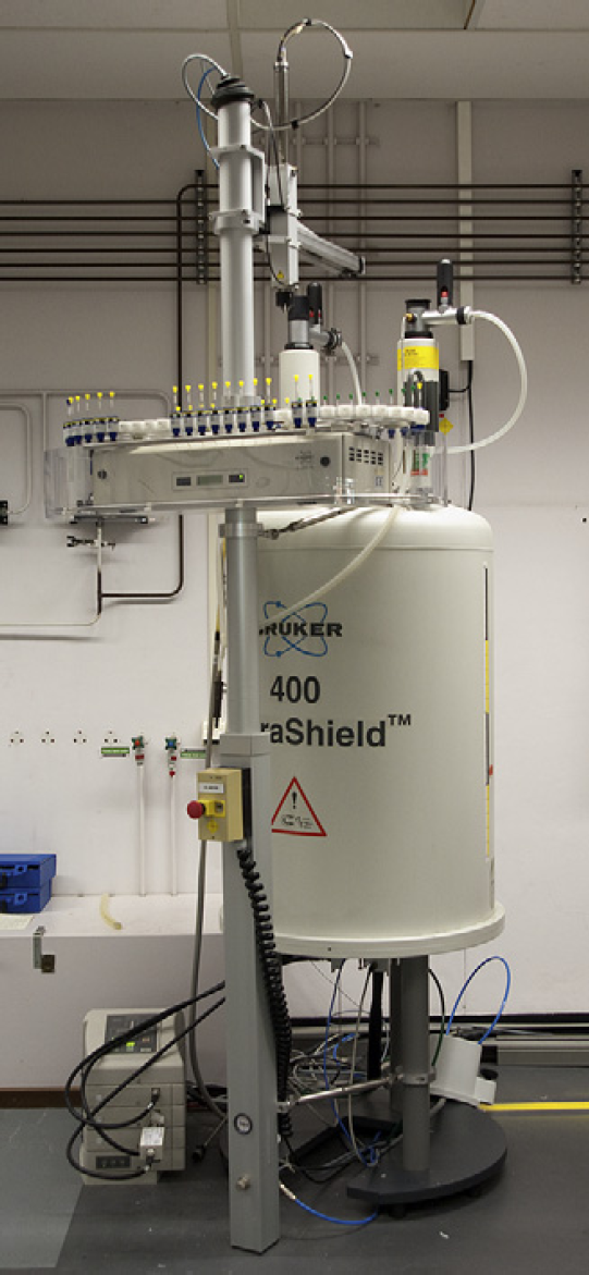
Bruker Avance 400 MHz spectrometer equipped with 60-position autosampler.
The operator workflow had evolved to be able to cope with this increased sample load. The operators used a variety of computer programs to deal with various data treatment steps and many templates to handle the different types of samples. Samples were processed in batches to minimize the opening and closing of computer programs and to reduce the need to change templates. While spending less time on actual NMR data processing, more and more time was consumed in transferring (intermediate) results from one application to another.
Figure 2 lists an overview of current workflow steps. Only those steps are mentioned that are performed for every sample. Before starting, one needs to have all of the following applications opened. Integral regions need to be defined and loaded into a NetNMR parameter file, 1 and a worksheet needs to be set up in Microsoft Excel spreadsheet software a that transforms the integration data into concentration numbers for repeat units and end groups. The right project in the laboratory database needs to be opened for the results to be entered. Thirteen process steps remain that are repeated for every sample and that require operator interaction. Some of these steps consist of more than just pressing a button. Phase correction and baseline correction may require zooming in on certain parts of the spectrum and manually adapting the phase correction and baseline correction parameters before applying them. Altogether, processing a sample requires about 100-mouse button clicks, 20 double clicks, and one- or two-dozen keystrokes. All of these are routine operations such as opening files and cut-and-paste actions that hardly require any specific NMR knowledge. The repetitive character of the operations easily leads to errors, and so it would be desirable to reduce their number.
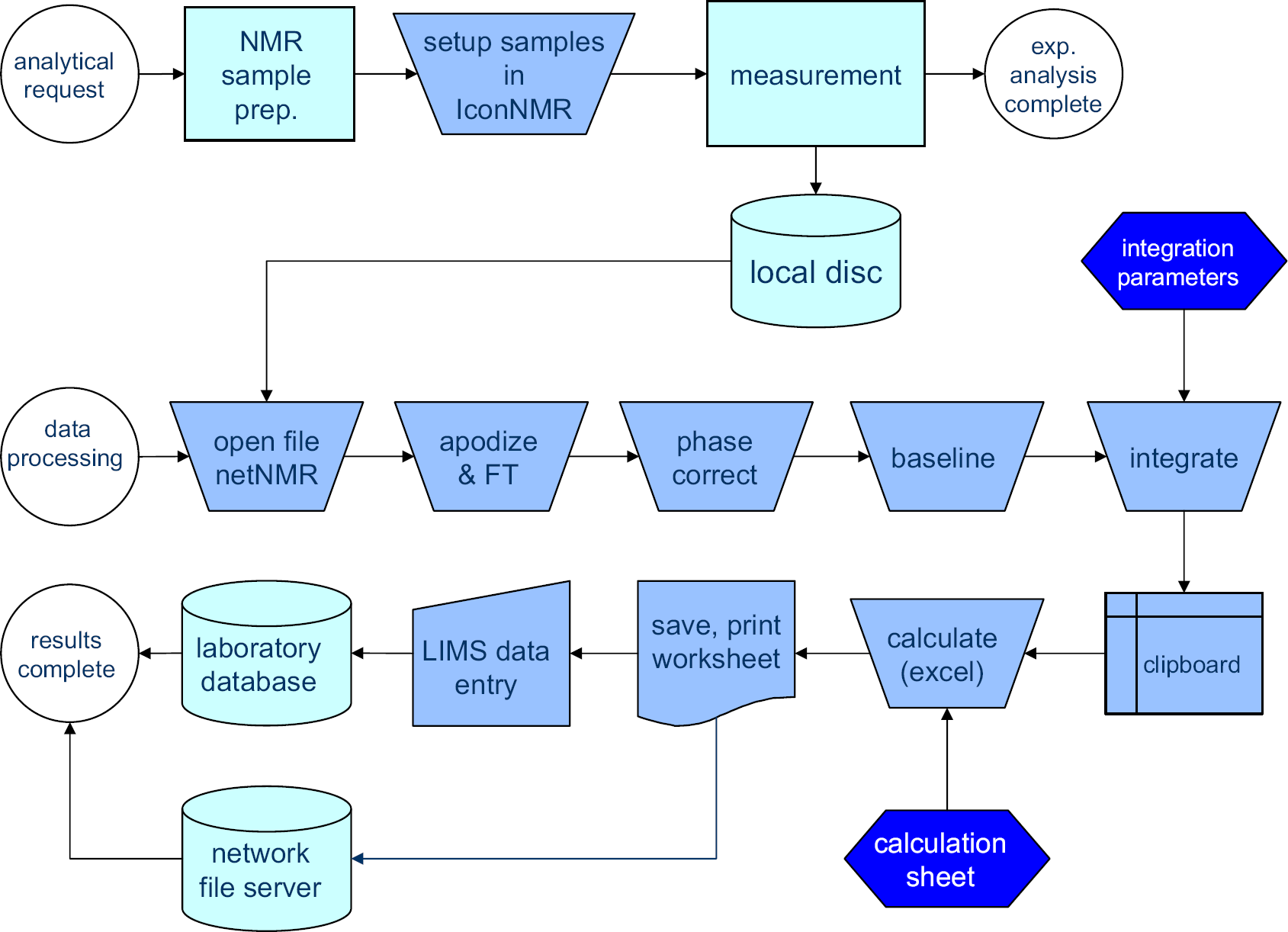
Old process of NMR analysis involving many steps in which manual input is required between “data processing” and “results complete.”
The projects that produce most of these copolymers were entering a stage in which the process chemistry was largely established and in which the process could be used as a rapid screening tool for the synthesis of new types of polymer backbones. Over a period of 2 years time, the number of different polymer backbones was going to increase from 5 to around 40. Reducing the number of analyses to be executed on each of these backbones to a bare minimum, the number of samples was still expected to double. Besides the increase in sample count and sample variety, a shorter feedback loop was needed for the product and process development teams, which meant that proper support of this development project required a reduction of the turn around time from an average of 6 days down to 1 or 2. This last requirement conflicts with the existing workflow of collecting and saving similar samples and processing them in batches. Either the resource level would need to be expanded significantly or the process should be automated to a large extent.
Table 1 shows the implications of both scenarios and compares them with the existing situation. Only the measurement of the routine samples is included in this analysis. The NMR device time is not a limiting factor, so only human resources are considered.
Two scenarios for meeting NMR support requirements compared against the current state
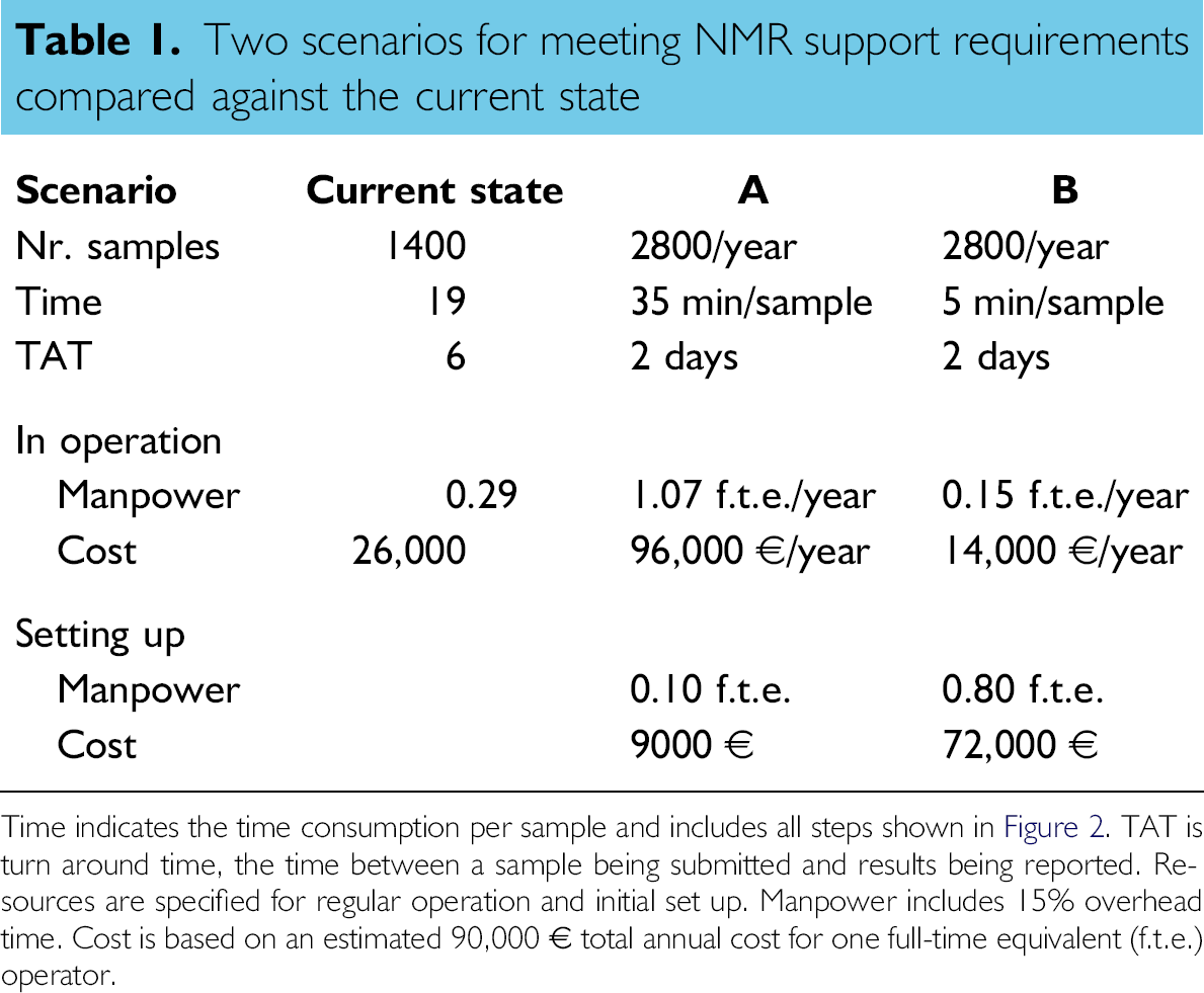
Time indicates the time consumption per sample and includes all steps shown in Figure 2.TAT is turn around time, the time between a sample being submitted and results being reported. Resources are specified for regular operation and initial set up. Manpower includes 15% overhead time. Cost is based on an estimated 90,000 € total annual cost for one full-time equivalent (f.t.e.) operator.
The current state shows that 1400 routine samples are processed annually, consuming about 19 min per sample. This situation has an average turn around time of 6 days. This leads to a time consumption of a fraction of 0.29 of a full-time equivalent (f.t.e.) of an operator (including 15% overhead), which in turn approximates a cost of 26,000 €.
In scenario A, the sample load is doubled. With a turn around time of 2 days, samples can only be processed individually or in small series leading to a reduced efficiency, which is expressed in the increased time consumption per sample of 35 min. The combined effect leads to a significant increase in the required resources to over an f.t.e. An additional (non-recurring) 0.10 f.t.e. is reserved for training and coordination in setting up this scenario.
Scenario B indicates the potential of an automation project. When data processing and results reporting are automated, only preparation of the sample and setting it up for measurement remain. This consumes 5 min per sample. Even when the sample count doubles, the resources required to do this are only half of those of the current situation. The programming and implementation took approximately 10 months and although slightly longer than anticipated, this does not drastically change the benefit of the project. The actual number of 0.80 f.t.e. resources for development has been used in the Table 1.
In summary, Table 1 shows that already in its first year, process automation (scenario B) compares favorably against scenario A and that this benefit will grow significantly in further years when the development costs have been digested.
We applied tools from the LEAN production philosophy 2 to analyze the process of Figure 2. The LEAN is a set of process improvement tools, originally developed by the Toyota Motor Corporation, that focus on recognizing and eliminating non—value-added process steps in a production process. 3 It labels non—value-added steps as muda, Japanese for waste, and categorizes this waste in seven different types, such as overproduction, waiting, motion, (over)processing, and rework. 4 Because these types of muda were originally defined in relation to production processes, some of them need to be reinterpreted when applied to electronic data processing. Overproduction, for instance, can refer to the fact that we not only store our results in the laboratory information management system (LIMS), but also in two different Excel spreadsheets for specific internal customers. In this way, more results, or duplicate results are produced that requires additional resources. Rework characterizes all of the efforts that need to be put in a defect product. In our NMR workflow, it refers to additional processing and verification of doubtful or erroneous results but also to actions taken by process and product developers based on faulty conclusions due to such results. Waiting needs no further explanation. Individual samples can remain in the queue for days to weeks because the operator tries to combine the data processing of similar samples in one batch to gain efficiency. Would he not do this then the waste in the shape of motion would be even more pronounced. In a physical process, motion is generated by the nonoptimal arrangement of machines, materials, and people, which requires the product or the worker to move further than necessary. The electronic equivalent is a nonoptimal process design, which relies on multiple computer applications and requires intermediate results to be carried over from one application to the other either through copying and pasting, saving and opening of files, or printing and reentering of information. This is the most prominent type of muda that is in our current process. The original request from the laboratory database is first printed. Sample names and descriptions are entered again in the NMR software. The test number is later on used by the operator to find the correct input location in the database. The file that is saved by the NMR software is opened in NetNMR. Integration values are transferred from NetNMR to an Excel spreadsheet using copy-and-paste operations, etc.
We would like to eliminate this motion and waiting type of muda by automating the entire process and moving from batch-wise sample processing to single piece flow in which each sample is processed individually, immediately after its raw data have become available. Also here, the LEAN methodology has an interesting approach, which is called autonomation. This is a form of intelligent automation that has human characteristics. It is focused on detecting (potential) errors early in the process and signaling them such that they can be resolved by human intervention before they end up in the product, or in our case in the analytical result. This approach is essential for our automated data processing to be successful for two reasons. Firstly, much skepticism existed around automation of this process, which is typically regarded as requiring an knowledgeable person to execute. All support for this project would be lost if the analytical results would be less reliable than before. The second reason why early detection of errors is important is that the end results (composition data) will typically not show whether or not an error occurred during the processing. This is something that the operator should signal during processing, for example, by observing unexpected peaks, peak shapes, or other peculiarities in the spectrum. This may explain the general assumption that a knowledgeable person is required to do the processing. The checks that an operator can do while processing the data can however easily be captured in software algorithms and executed during data processing such that potentially erroneous results are not copied into the database, in line with the concept of autonomation or jidoka as it is called in Japanese. Although there are some capabilities for automated data processing incorporated in the NMR software that we had available, they were insufficiently flexible to capture the human intelligence of autonomation. For this reason, we proceeded to develop our own software solution. The key requirement is that the reliability of results should be equal or better than in the current situation. The goal is to maximize productivity and to minimize operator workload by eliminating as much muda as possible, ideally replacing all the steps in between the NMR software and the laboratory database by an automated process.
The following sections describe the automation framework program and the technical details of its inner processes. The Performance and Conclusions section toward the end will summarize the results in a broader perspective including the various muda types.
Experimental
The NMR spectra are recorded on a Bruker Avance 400 MHz machine equipped with a 5-mm QNP probehead. One hundred twenty eight scans were applied using a 30° flip angle pulse, 2.56s acquisition time, and 10s recycle delay. The temperature controller was set at 44 °C. Samples were measured at a concentration of 50–70 mg/mL in a deuterated solvent, typically CDCl3.
The NMR computer was equipped with Hummingbird Exceed to run the Unix-based NMR-Suite 3.5 software package from Bruker Biospin, including Icon NMR 3.5.6 and XWin-NMR 3.5. The computer had Microsoft Excel 2000 (v9.0.8968 SP-3) spreadsheet software and Adobe Reader (v7.0.9) installed.
Data-processing routines were developed in Matlab (v7.3.0/R2006b). A compiled stand-alone executable file was generated using the Matlab Compiler (v4.5/R2006b). The executable was copied onto the NMR workstation and programmed to run automatically several times a day using the “Scheduled Tasks” feature of the Windows XP operating system.
Complex free induction decay (FID) signals were extracted from the raw data files using selected routines from the matNMR software package, 5 which is distributed under an open source license. An apodization of 0.3 Hz was applied to the FID before subjecting it to the phase correction algorithm. 6
The NMR workstation was connected to a data fileserver from which another workstation running Labware Labstation takes care of the upload of data into the Labware LIMS (v5.02j+) database system. Results are submitted in the form of a standardized comma-separated-values file, which is generated by our software. This file is picked up by the Labware Labstation LIMS parser scheduler, which runs every 15 min. Results that are uploaded are automatically approved within LIMS because a more stringent approval process has already taken place in the form of the manual or automated approval that has been discussed in this article.
Automation Framework
The Matlab programming environment was used to develop a set of automation routines to cope with the entire workflow from the point of accessing the raw NMR data on disk up to results validation and entry into the laboratory database. A high-level overview of the automation framework is given in Figure 3. The Matlab programming environment was selected because of the ease with which it handles large sets of data, such as NMR spectra, but also because of its built in file-handling capabilities, including the ability to generate files, which can be read with Excel spreadsheet software and to save documents in the portable document format (PDF), which are easily read by Adobe Reader. Files of these types are used to interface with the operator.
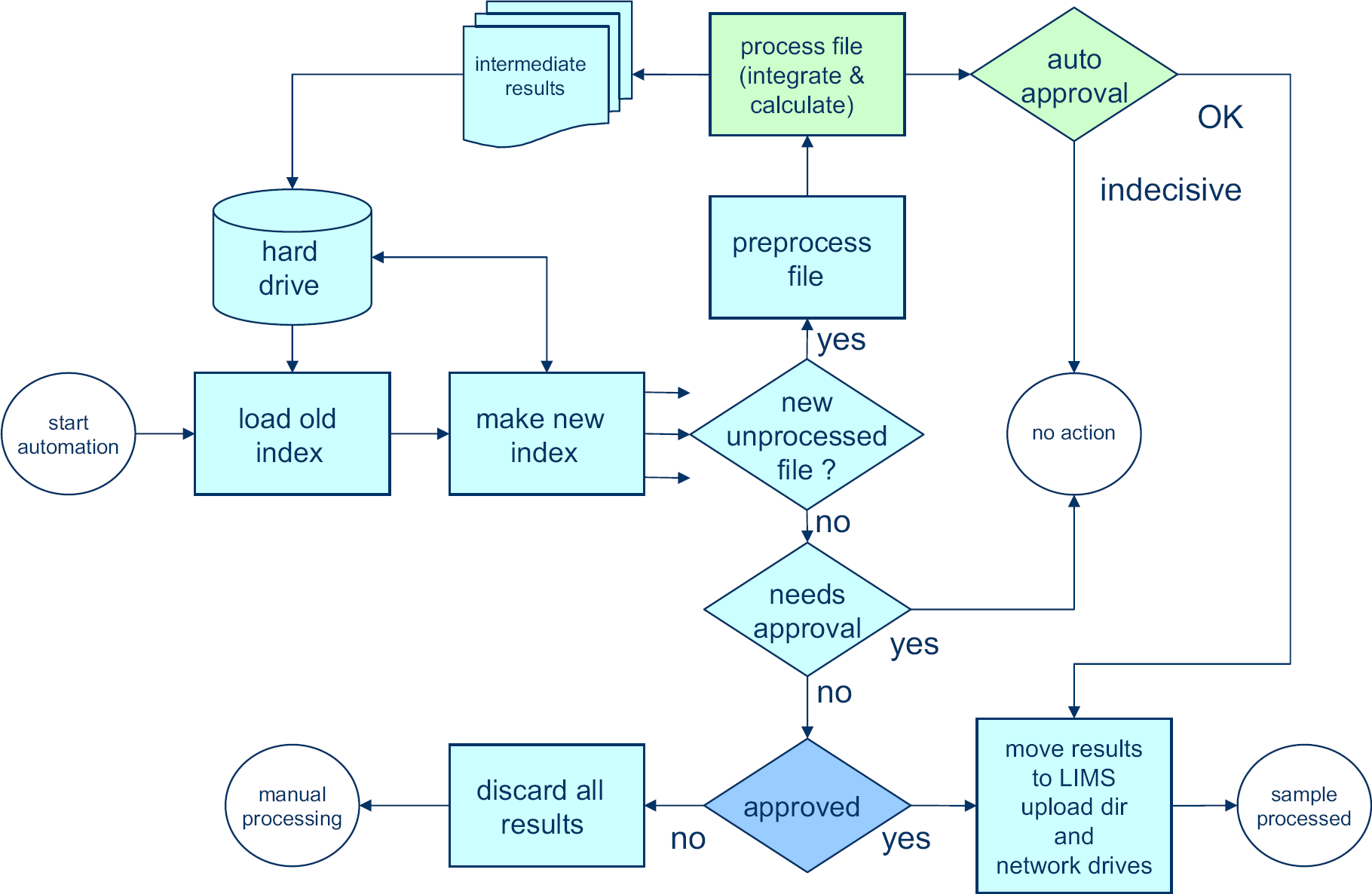
New automated data-processing process that replaces the manual processing part of Figure 2. No manual input is required. When data can be automatically approved by the software, results are reported and stored in the laboratory database. Integration and autoapproval (green) are backbone specific. The other steps (blue) are identical for all samples.
When the automation routines are executed, the system starts by updating its administration. There is an Excel spreadsheet software document on the hard disk drive (HDD), which lists the status of each data file on disk from the previous time that the automation was run (Fig. 4). This index indicates whether a data file was already processed or not and whether the results have been approved, rejected, or if approval still needs to take place.
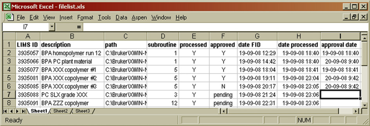
Contents of the hard disk drive index file. The LIMS ID number is used as the sample name in the Icon NMR software package. The path contains a subfolder that indicates the type of polymer, for example, 01 for bisphenol acetone (BPA) polycarbonate, which is then processed using integration parameters of subroutine 1. The processed and approved columns indicate the status of the analytical results. 7
The automation program iterates through the data folders on the HDD and generates a fresh list of data files. Any file that is not present in the Excel spreadsheet software document is given the “unprocessed” label. These are new files, which were not present on disk the last time the automation ran. The new list then replaces the old. For all unprocessed files, the automation attempts to process them. There are two possible outcomes, which we will call routes:
Processing is successful. The software is able to verify this in the autoapproval process, submits the results to the LIMS database, and posts reports to other network drives. The file is marked as completed and processed (bucket III, Figure 5) in the HDD index and will not be touched again by the automation process.
Classification of datafiles in the hard disk drive index. Each file falls in one of four buckets indicated by I-IV.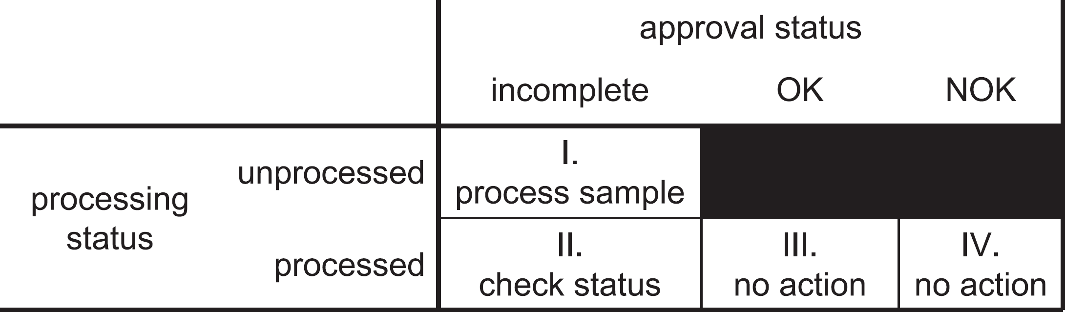
Processing is successful, but the autoapproval routine is insufficiently certain to approve the results. The file is marked as processed but requiring approval (bucket II, (Fig. 5) in the HDD index, and next time the automation process runs it will check to see whether the approval status in the intermediate results file has been changed by the operator.
Apart from working on the new and unprocessed files, the automation also looks at the files in bucket II, those which have been processed and are marked requiring approval. When such a file is encountered, the automation routine looks into the intermediate result files for the sample. The result files also contain an approval status field and this is the place where an operator would set the approval status after having inspected the results. There are three possible routes:
The file is still found to be “pending approval.” No action is taken. The file remains in bucket II, and it will be checked again next time the program is run.
The file is found to be approved. Result files are moved to their final destination (LIMS import folder, network drives) or disposed (PDF files with spectra for visual inspection). The datafile is marked as “approved” in the HDD index. Nothing will happen to the file anymore in the automation process (bucket III, (Fig. 5).
The file is found to be disapproved. No entry is made in LIMS. The datafile is marked as “disapproved” in the HDD index. Nothing will happen to the file anymore in the automation process (bucket IV, Fig. 5). Note that no results have been produced and the operator will need to consider reanalyzing the sample or processing the data manually, depending on the root cause of the rejection of the results.
The preferred route for any sample is route 1. When such a sample has been placed in the autosampler and entered in the queue of the NMR software (Bruker IconNMR), it requires no further attention from the operator other than disposing of the sample after the analysis has been completed. The results will be made accessible to the requestor through the database automatically. If automated approval is not possible, route 2 is taken and subsequently route 3 until a visual inspection of the results has either led to approving the results (route 4) or rejecting them (route 5). As long as the operator does not decide on approval, the sample will keep following route 3 when the automation runs.
Typical examples of samples that are not automatically approved are those with contaminations (peaks appearing in places not expected by the software) or samples being recorded under the assumption of being a different sample. When a polymethyl methacrylate (PMMA) sample is submitted as being a bisphenol acetone (BPA)-based polycarbonate (PC), the automated processing will not yield sensible results. If visual inspection shows that the results can still be used, the sample can manually be flagged as approved after which results will be automatically processed. The approval process itself is detailed further on in this article. Otherwise, when the sample is disapproved, it is no longer considered by the automation and should either be completely reprocessed manually or be rerecorded if there is an anomaly in the spectrum.
When we compare the scheme of the old workflow (Fig. 2)) with the one representing the new workflow (Fig. 3), most of the manual steps have been eliminated. Consider however that during all of the manual processing, two types of information were required from the operator for which we will need to think of a way of supplying them in the automated environment. To prevent the need for any additional human intervention, this needs to be done during the sample setup in IconNMR, which is the single remaining nonautomated step in the process.
Firstly, the operator would know what type of polymer was being analyzed, and based on that apply certain integration parameters and calculation steps. It does not make sense to look for hydroxy functional end groups in polymethyl methacrylate nor does looking for a methyl ester moiety in the repeat unit of BPA polycarbonate. The automation routines can easily apply different integrals and calculations to different polymer families. Different folders are used to indicate this. PC data files are stored in subfolder 01, PMMA files in subfolder 02, etc. Column D in Figure 4 lists the subroutine that is used for the integration based on the deepest subfolder in the file path.
Secondly, the operator would know where to store the results in the LIMS. For every NMR analysis that is requested, a unique test number is generated in LIMS. This test number is used as the sample filename. This automatically ensures unique filenames for all samples (column A, Fig. 4).
The description field in IconNMR is used to provide a meaningful sample description. This is copied to the intermediate result files and to the HDD index (column B, Fig. 4) such that upon visual inspection (if needed) the operator has certain background information to help decide whether the results make sense or not.
The framework has been programmed in such a way that it is flexible and easily scalable. Different types of polymer backbones can be added to the program without modifying any of the routines, which are not backbone specific (green blocks in Fig. 3). When a new, two-digit subfolder is found in the list of NMR data, the program automatically recognizes this and looks for a corresponding data-processing routine and reference spectrum. These are the two things that need to be added for a new backbone type. The results are then automatically matched with the appropriate fields in the LIMS laboratory database, based on the results description. When the integration routine specifies for instance that BPA is a monomer in a particular backbone, it automatically recognizes that the result of “20ppm” with the label “BPAOH” needs to be stored in the LIMS field “OH end-group, monomer 1” if BPA is the first or the only monomer listed. By limiting the hard coding in the framework routines, there is no need to tamper with any of this code when adding additional polymer backbones and code writing is purely restricted to the new integration routine.
Preprocessing
The preprocessing block, as shown in Figure 3 contains a number of general steps. The filename, test number, and subfolder are passed to the main processing routine. First, the FID and the analysis parameters are extracted from the data files on disk using available open source routines. 6 Next, an apodization is applied to the FID (0.3 Hz), and the Bruker digital filter is removed. 6 After Fourier transformation, a complex spectrum is obtained. Phase correction of the complex spectrum to obtain the absorption spectrum is a crucial next step. This is typically done by adjusting two parameters, the zeroth and first-order phase correction angles, in such a way that that an optimal spectrum is obtained: peaks are narrow, symmetrical, and point upward, and the baseline area between peaks is smooth. It is relatively easy to develop a routine that returns approximate values for the phase-correction parameters, but more development work was needed to design a method that gives very accurate results in a robust manner. 7 This was necessary to be able to use the spectrum quantitatively. Once a proper absorption spectrum is obtained, integration is performed and the integral numbers are used to calculate the composition of repeat units and end groups.
Integration and Calculation
The integration and calculation routines from the processing block (Fig. 3) are unique to the various sample families and are chosen based on the subfolder in which the data file is stored. Processing follows the scheme of Figure 6
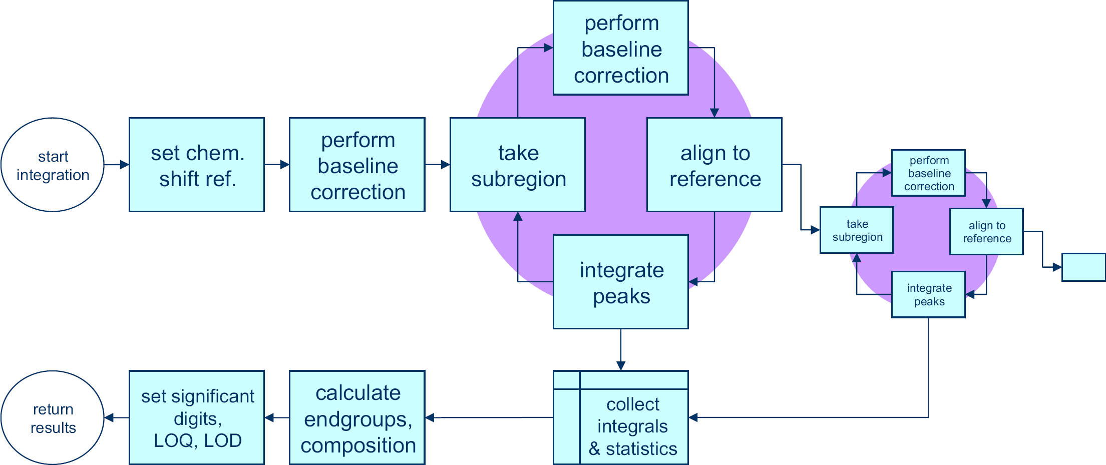
The spectrum is first shifted horizontally such that the position of a reference peak is in the correct position. Typically, trimethyl silane a compound added to deuterated chloroform is used for this purpose, but other solvent or polymer peaks may also be used.
Next, a full spectrum baseline correction is performed according to the method of Golotvin and Williams. 8 This method is discussed in the next section. Once this is complete, a cycle is run, started by selecting a subregion of the spectrum, applying a baseline correction to it, aligning it with that same subregion in a reference spectrum to correct for any peak shifts, and then integrating the peak as required. The integration step produces one or more integral values and both the integration and the alignment yield parameters that describe these processes. All of these values are collected. When a subregion is finished, another subregion can be taken from within the first subregion, thereby zooming in further on individual peaks or a new subregion can be defined in the complete spectrum. The advantage of zooming in on a certain peak in a number of steps is that baseline and alignment parameters can be optimized at every level, leading to a more robust process than directly taking each individual peak from the complete spectrum. This allows for more sophisticated processing of overlapping peaks for instance.
Once all the integrals and process parameters have been collected, the component analysis is performed that gives all of the relevant results, such as composition and end groups. These results are checked against detection and quantification limits that apply and then returned to the main automation framework, together with the process parameters of the integration and alignment processes.
Baseline Correction
The method that was used is the baseline recognition method described by Golotvin and Williams. 8 First, the standard deviation of the noise is determined by dividing the spectrum in a number of regions (n) and by determining the standard deviation of the signal in each of these regions. It is then assumed that there is at least one region that is free of peaks and consists of noise only. The lowest standard deviation in the set is therefore assumed to be that of the noise (σnoise). Figure 7 shows six windows in this spectral subregion containing signals of aromatic alcohols. The rightmost window has the lowest standard deviation, of 0.27 in this case.
First, the standard deviation of the noise is determined by dividing the spectrum in a set of n areas and determining the standard deviation in each of them. This assumes that at least one area is present that is free of peaks. In this case, the lowest s is that of the right window with a value of 0.27.
Every point in the spectrum is then evaluated to see whether it should be considered a baseline point or a “peak point.” The point is considered to be in the center of a window with a specific width (w). In this window, the signal range that is spanned by the spectrum is determined by subtracting the minimum value from the maximum value within that window. If this range is smaller than a constant (K) times the standard deviation of the noise, the point is considered to be a baseline point, otherwise the point is considered a “peak point.” Figure 8 illustrates the evaluation of two data points. In this case, width w = 30 and factor K = 6. Because the range around the left point (0.26) is smaller than 6 × 0.27 = 1.62, this point is considered to be part of the baseline. The right point is part of a peak because the range around it is larger than 1.62. Therefore, this last point will not be used when fitting a polynomial baseline. With all the baseline points identified, a baseline is generated by fitting a line or curve through these points and subtracting the fitted curve from the spectrum.
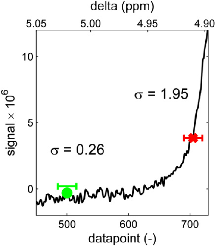
Every point in the spectrum is then evaluated by calculating the standard deviation of the spectrum in a window (width w) around it and comparing the standard deviation with that of the noise, multiplied by a factor K.
Note that this baseline routine takes four input parameters:
The number of regions used in determining the standard deviation of the noise (n)
The window width used for evaluating points (w)
A constant K to multiply with σnoise to form the threshold distinguishing peaks from baseline, and
The order of the fitted baseline (p).
As shown in Figure 9–Figure 12 the parameters can be tailored to a wide variety of baseline problems making this approach applicable to spectra with different signal-to-noise ratios.
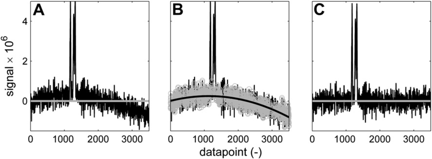
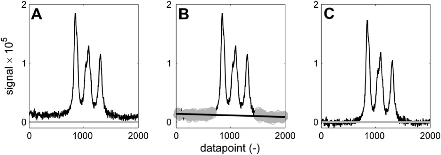
Baseline correction of a noisy curved baseline. n = 200; w = 30; K = 4; p = 2. (A) Spectrum before correction. (B) Baseline points (gray) and second-order polynomial fit (black). (C) Corrected spectrum.
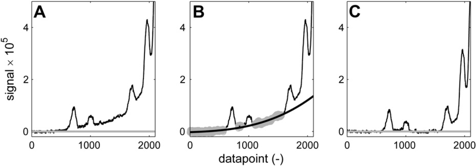
Baseline correction of peaks on the tail of a bigger signal. n = 200; w = 100; K = 8; p = 3. (A) Spectrum before correction. (B) Baseline points (gray) and third-order polynomial fit (black). (C) Corrected spectrum.
It is interesting to see in Figure 11 and Figure 12 how different sets of parameters can give different results on the same part of the spectrum. If the bump underneath the three broad peaks is considered to be a baseline artifact, then the aggressive set of baseline recognition parameters that is used in Figure 11 manages to find baseline points in between the three peaks. The sixth-order polynomial curve that is fitted effectively eliminates the bump, resulting in three baseline separated peaks, which can be integrated without the additional bump area. If the bump is considered to be generated by the superposition of the three peaks, then its area should not be eliminated. A more conservative set of baseline selection parameters in combination with a linear fit results in the spectrum of Figure 12C, which has the offset that was present in Figure 12A eliminated, but has left the bump intact.
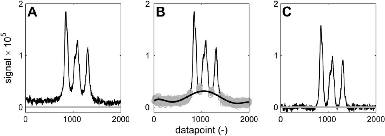
Baseline correction of broad peaks. Using these parameters: n = 200; w = 40; K = 6; p = 6, the curvature underneath the peaks is considered an artifact and eliminated by the baseline correction. Three baseline-separated peaks are returned. (A) Spectrum before correction. (B) Baseline points (gray) and sixth-order polynomial fit (black). (C) Corrected spectrum.
Baseline correction of broad peaks. Using these parameters: n = 200; w = 130; K = 7; p = 1. (A) Spectrum before correction. (B) Baseline points (gray) and linear fit (black). (C) Corrected spectrum.
One thing that this baseline correction method is not suited for, however is the isolation of small or broad peaks on steep slopes, for example, of another bigger peak. An example is shown in Figure 13. In this case, a different routine is used that fits a polynomial of specified order through a set of local minima that is found in a number of specified ranges. Figure 13B indicates nine ranges (each one specified by two x coordinates) that are passed to the baseline correction routine in the form of an array. The ranges are indicated by the horizontal black bars (their vertical position is arbitrary). In each of these ranges, the local minimum in the spectrum is selected as a baseline point (gray points in Fig. 13B), which is used to fit a polynomial. By working with ranges rather than points with a fixed position on the X-axis, a certain flexibility against shifting peak positions is incorporated. By using these ranges, one ensures that baseline points are selected in specific areas of the spectrum, which would not be possible with any given set of fixed parameters by the aforementioned approach. In this case, a third-order polynomial baseline correction results in the spectrum of Figure 13C, which allows each of the three smaller peaks to be integrated. To prevent certain baseline artifacts, the baseline correction based on these local minima can also be executed using linear interpolation between adjacent local minima rather than a polynomial fit through the entire set of baseline points.
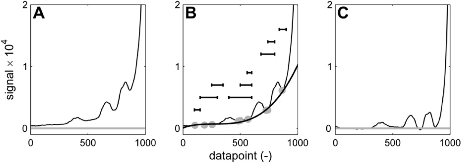
Baseline correction to isolate small or broad peaks on a steep slope is achieved by picking minima within certain predefined ranges (indicated by the horizontal lines in (B)) and fitting a polynomial through these points or applying linear interpolation between them. The approach with ranges gives a certain tolerance to variations in peak position, peak width, and slope steepness. (A) Spectrum before correction. (B) Baseline points (gray) and third-order polynomial fit (black). (C) Corrected spectrum.
Signal Alignment
Due to several reasons, the exact peak position of a signal may vary in NMR. Particularly, sensitive are signals from protons that participate in hydrogen bridges such as —OH or —NH2. These groups give broad signals and their position varies with overall sample polarity. Therefore, traces of water or the concentration of polar groups may shift the peaks.
Also, peak overlap may influence peak position. When two peaks partly overlap, the position of their maxima will vary with the relative magnitude of each of the two or more signals.
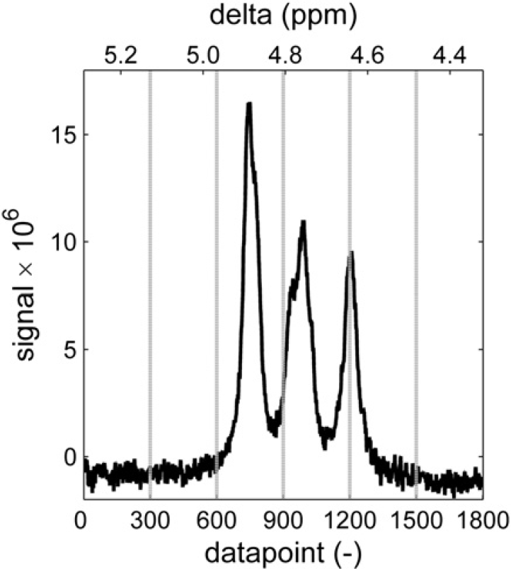
To ensure that peaks are integrated correctly, the part of the spectrum that is being processed is first aligned to the same fragment of a reference spectrum. The reference spectrum is typically a spectrum from a sample with a representative composition, that is, nonextreme values for end groups and composition. The alignment is achieved by minimizing the sum of squares of the difference between the reference signal and the sample signal after normalizing both to a fixed maximum peak height. 9 Minimization is done while shifting the sample spectrum along the chemical shift axes. Figure 14 (top, gray) shows part of a reference spectrum. The vertical dotted lines indicate the integral areas, which are needed to determine the integral area of the peaks. Below the reference spectrum, a sample spectrum is shown (black). Obviously, this spectrum is somewhat shifted. If this spectrum would be integrated using the integration limits as they have been set on the reference spectrum, the results would not make sense. The left integral would not cover the left peak completely, resulting in an artificially low value, whereas the second integral would have an artificially high value caused by the left peak. The sum of square difference between the spectrum and the reference spectrum is plotted in Figure 15. The minimum is found when the spectrum is shifted 53 points to the left. According to Figure 14 (gray, bottom), this aligns each of the three peaks correctly with the reference spectrum. Now the integration limits as they have been set using the reference spectrum can be applied to the sample spectrum. The maximum allowed shift can be passed to the alignment routine. This speeds up the routine and prevents unrealistically large shifts, which could, by chance, result in a mathematically preferred situation. Besides the shifted spectrum, the alignment routine returns the number of data points of the applied shift and the correlation coefficient between the shifted sample spectrum and the reference spectrum. Although these values are not uploaded into the laboratory database or reported, they are stored by the automation software and used in the automated approval of spectra, which will be discussed later on.
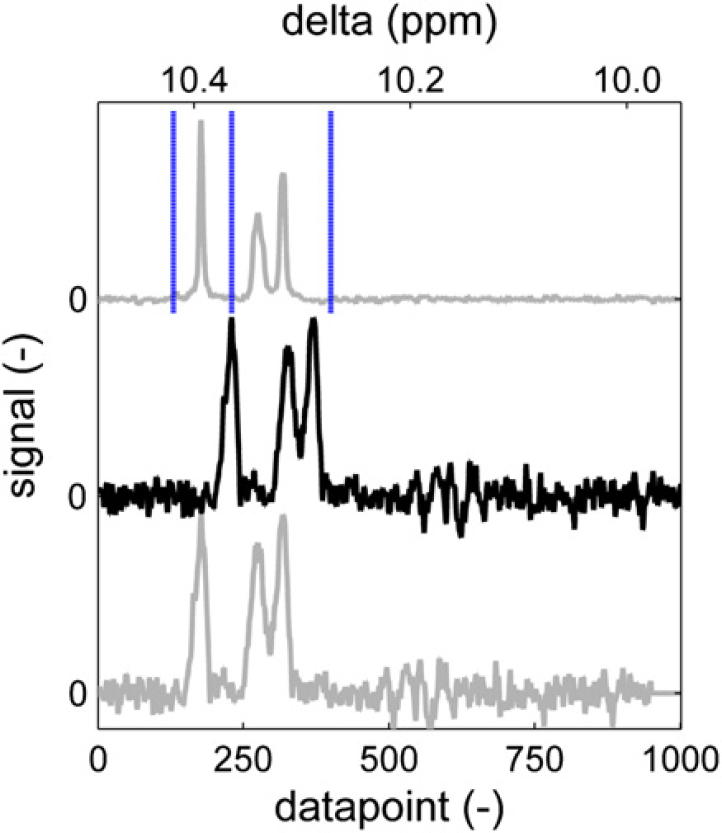
Reference spectrum area with integration limits (top). Sample spectrum with shifted peaks (middle). Sample spectrum aligned to reference (bottom).
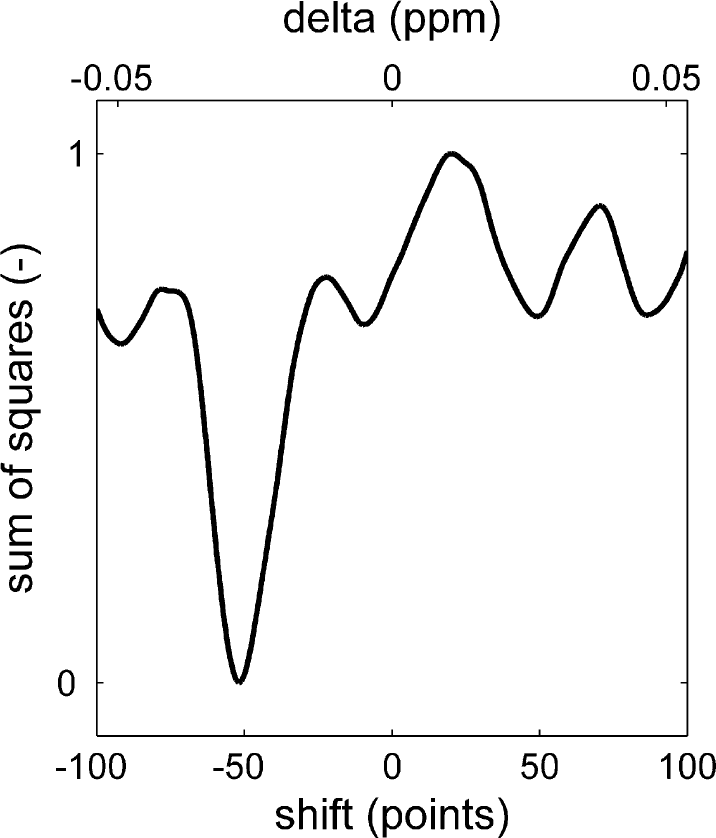
Sum of squares of the difference between the reference spectrum and the sample spectrum as a function of its horizontal shift.
The routine takes a point range as input parameter that is used for the evaluation of the sum of square difference. This allows the edges of the spectrum, which do not contain any signal due to the spectrum shift, to be excluded from the calculation.
The spectrum alignment approach works well under most circumstances. The only exception is encountered when a set of peaks needs to be aligned with significant variation in peak heights between the sample and the reference spectrum. In some occasions, the benefit of aligning the largest peak in the spectrum with the largest peak in the reference spectrum (in terms of sum of square contribution) can be larger than the penalty for misaligning the remainder of the spectrum. In such cases, a more sophisticated pattern recognition approach is used.
Figure 16 shows the methyl proton signal of BPA. The reference spectrum (a) has a main peak that originates from BPA units, which are incorporated in the polymer chain, surrounded by two carbonate units. To the right of the main peak is a second one, which corresponds to BPA units at the polymer chain end in which one of the phenyl rings has hydroxy attached to it, whereas the other has a carbonate unit. Hardly visible is a third peak, which originates from un-reacted BPA with two hydroxy groups attached to the phenyl rings. This is a typical pattern for a polymer sample. Sample spectrum (b) is somewhat different. It is the BPA methyl signal from an oligomer sample taken at approximately 60% conversion. In such a sample, the main peak originates from BPA at chain ends. To align the spectrum correctly, a 20-point left shift would be appropriate. The result of the alignment routine is shown in spectrum (c). The most favorable sum of square difference is apparently attained by matching the higher peak in the sample to the higher peak in the reference although this causes misalignment of the monomer peak and of the bisubstituted BPA peak. Using the misaligned spectrum to calculate BPA conversion will yield erroneous information. In this case, 93% conversion is calculated from the misaligned spectrum and 68% from the correctly aligned spectrum.
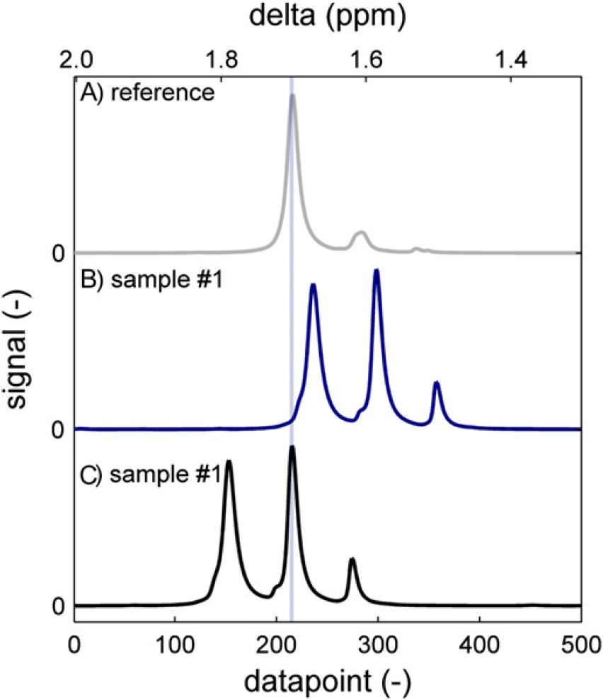
The methyl region of bisphenol acetone (BPA) PC around 1.67 ppm. The reference spectrum (A) has a main peak that corresponds to a midchain BPA unit. Sample spectrum (B) is of a low molecular weight oligomer, which has additional signals from chain-end BPA and unreacted BPA and has peaks shifted toward the right. (C) Automatic alignment minimizing the sum of square difference leads to erroneous results.
To prevent these misalignments, one could generate a specific integration routine for this kind of samples. This is sometimes useful but on many occasions, it is not possible to predict, to which specific routine a sample should then be submitted. A second option is to restrict the maximum allowed shift to such a low number that a shift of 83 points, which was applied in this case, is not possible. A third option is to require sum of square improvements during the entire shifting procedure, such that a local minimum will be found. In the case of the spectrum in Figure 14, this would lead to a left shift of 10 data points (see Fig. 15) rather than the optimum 52-point left shift. All three options are used where applicable, but also occasions remain in which such solutions are not applicable. This is when we revert to pattern recognition.
Pattern Recognition
The pattern recognition algorithm that we use identifies local maxima by moving a window across the spectrum and recording the local maximum in the window, provided it is not the leftmost or rightmost point in the window. This prevents points on a slope being added to the list of maxima. The window size can be specified and should be approximately equal to the expected width of the narrowest peak of interest. When a window of 20 points width is dragged across a spectrum, every data point has 18 chances of being considered a maximum (the two situations in which it is on the edge of the window being excluded). Only points with this maximum score are added to the shortlist for further consideration. For the spectral range of Figure 16, this typically results in 4–8 “peaks.”
The shortlist of identified peaks is then used to generate a matrix of interpeak distances, which are then sorted in a list according to the product value of the signal height of the two peaks in each pair. Here, one can apply a size criterion to filter out noise, for instance removing any peak pair for which the signal product value is less than 1% of that of the biggest entry in the list. For the spectral range of Figure 16, this typically leaves only 1–3 peak pairs.
Now the program will need to be instructed what to do with these peaks. In the example of the BPA methyl signal we found that of the three peaks, the leftmost one (the bisubstituted BPA) is always present. If no “peak pairs” are found, the spectrum is returned with this one peak in the fixed position of datapoint #210. If there are more peaks, the distance between the left and the middle peak was found to be 64–75 data points. The distance between the middle and the right peak was in the range of 60–68 data points. As the two interpeak distances are overlapping ranges, this information as such is insufficient to track a specific peak. Therefore, the program is instructed to look for peak pairs, which are 64–75 data points apart. When more than one of such sets is found, the leftmost one is taken and a part of the spectrum is returned that has the left peak of the set in the fixed position of data point #210. After this approach, we found that samples taken in a broad conversion range could be aligned properly (Fig. 17). Interpeak distances and other parameters can be passed to the routine to optimize performance in other situations.
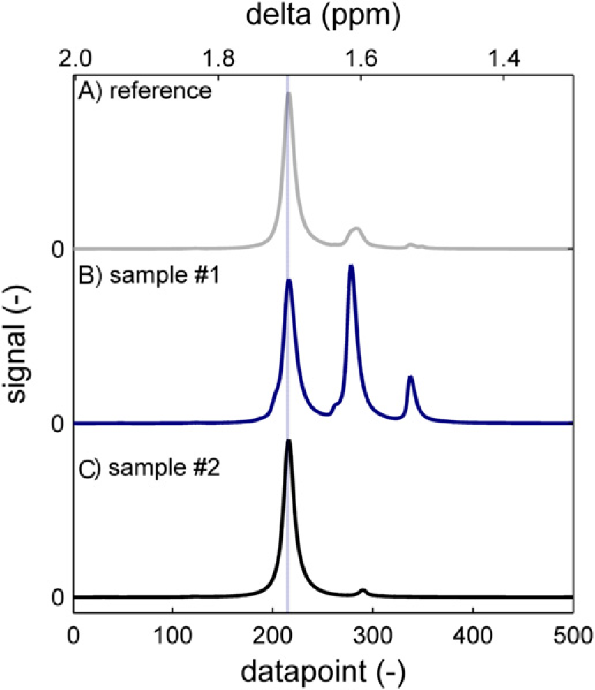
The methyl region of bisphenol acetone (BPA) PC around 1.67 ppm. Both an oligomer sample (B) and a high-polymer sample (C) are correctly aligned to the reference (A) using pattern recognition techniques.
Integration
Once the spectrum has been correctly aligned to the reference spectrum, the integration consists of summation of the data points between the integration limits as they have been set on the reference spectrum. As all data points of the spectrum are equidistant in frequency/chemical shift, there is no need to consider X-axis units. Besides the value for the integral between the integration limits, the percentage of the integral versus the total signal in the spectrum (fragment) is returned. This is again a number that is used to judge the validity of the result. If there is an anomaly in the sample that gives rise to additional peaks, this value will be lowered.
When the values for all of the integrals of interest are collected, the relevant properties for the sample are calculated. These are typically expressed as a molar percentage relative to the total amount of monomer. For BPA-based polycarbonate, for instance, OH end groups are expressed relative to the number of BPA repeat units.
Approval
Manual Approval
The results of the integration and calculation are stored locally on the computer of the NMR spectrometer in a dedicated folder. When the autoapproval process is not active, or when the autoapproval process cannot approve the results, the process in Figure 3 ends at the “no action” end point. Autoapproval is only enabled for a specific polymer family when a substantial amount of spectra has been processed and when statistical analysis has shown that automated approval is feasible. For every new polymer type that is added to the automation process, manual/visual approval is the starting point.
When the automation process is run again, the sample that has just been processed is no longer considered as a new file (Fig. 3) and when it is not manually flagged as approved or rejected, the process ends at the same “no action” end point. This means that the sample results remain inactive until the approval flag is manually set in the folder containing the intermediate results.
When this has been done, the process follows the path downward and depending on the verdict of the operator (approved/rejected), the results are either discarded or they are reported to the laboratory database and a network location. In both cases, the local folder is cleaned such that graphs and other intermediate results are removed and only one set of the numerical results and the statistics of the processing remain. This latter information can be used to set up the autoapproval process.
An overview of the intermediate results is shown in Figures 18 and Figure 19. Several graphs stored in PDF files summarize the phase correction and integration process and allow comparison of all relevant regions in a spectrum with those in a reference spectrum. An example of such a graph is shown in Figure 20, which is the six-proton methyl signal of the BPA repeat unit around 1.67 ppm. The height normalized sample spectrum is overlaid on the reference spectrum. No particular differences are observed. When all regions in the spectrum produce plots like this, the results are accepted. The vertical blue lines indicate the integration limits. Numerical results are summarized in a data file in commaseparated-values format. This file is suitable for processing by the LIMS autoupload parser of the laboratory database. On approval of the results, the CSV file only needs to be moved to the right upload location. Finally, there is an Excel spreadsheet software file, which contains the numerical results together with the sample ID and description and the approval status. Approving or rejecting sample results requires nothing more than putting a Y or N character in cell B4, respectively. After completion of the approval process, the files of Figure 18 are discarded. What remains is simply the status of the sample in the HDD index file (Fig. 4). This Excel spreadsheet software document keeps track of which samples have been processed and approved or rejected to be able to distinguish new files from existing ones and to identify files requiring approval. Both pieces of information are needed to guide samples through the flow diagram of Figure 3.
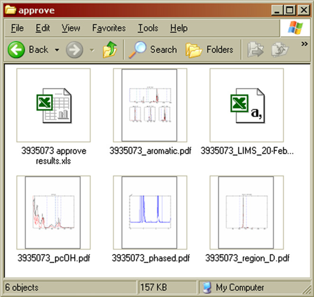
Intermediate results stored locally on the NMR computer while waiting for approval. 7
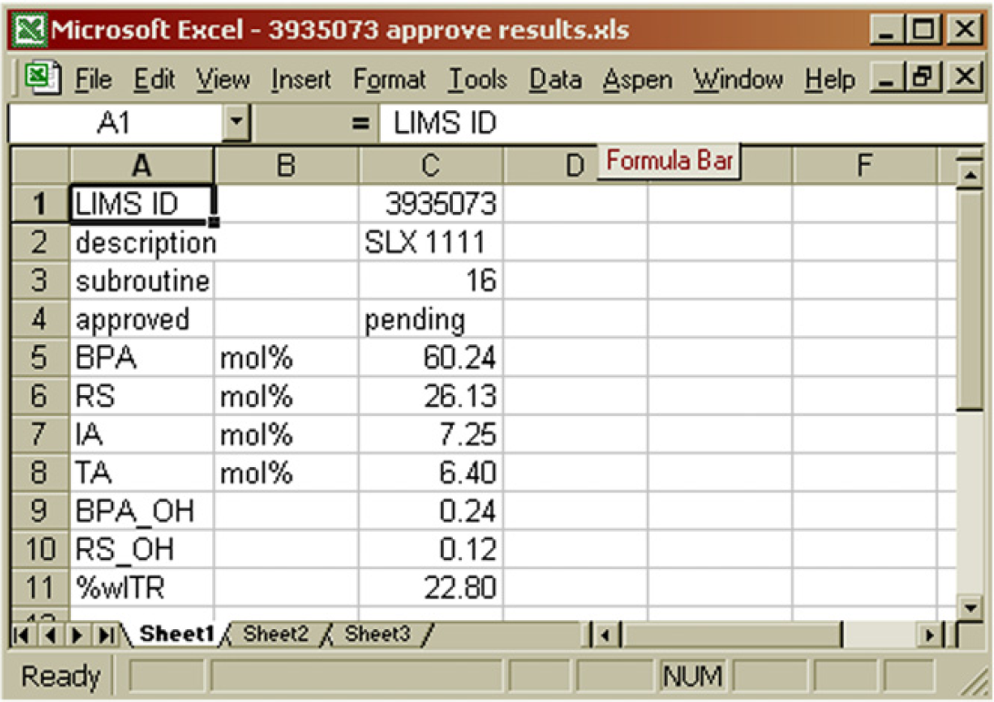
Contents of the “approve results” file. Manual approval is achieved by replacing “pending” in B4 with either Y or N. 7
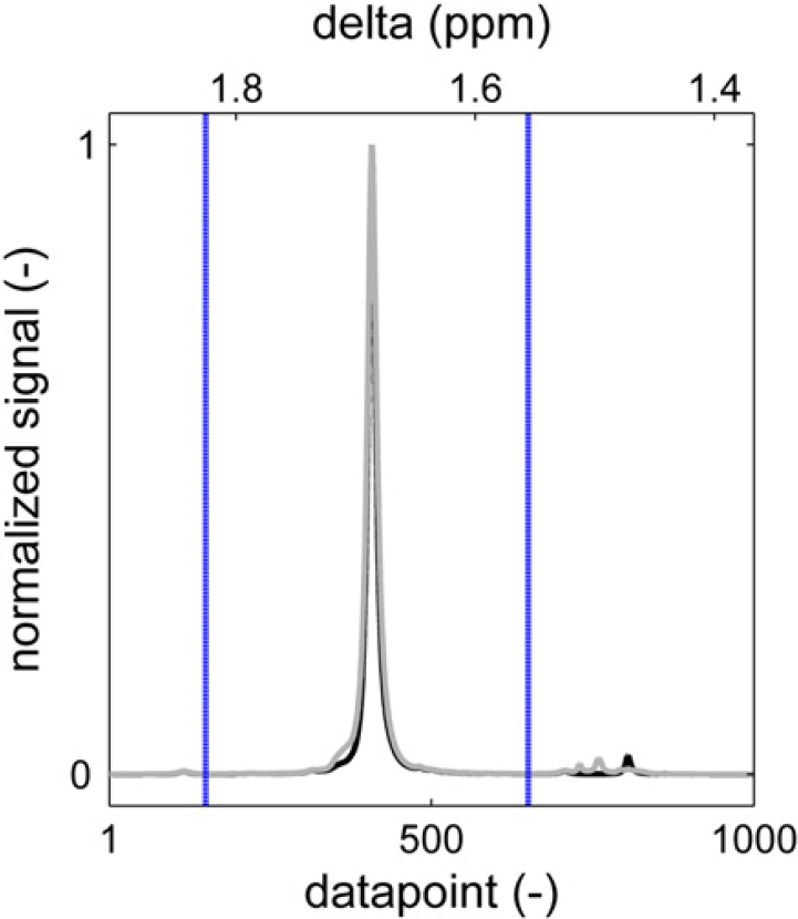
Sample content of a graphical results file. The height normalized sample spectrum (gray) is plotted over a reference spectrum (black) after baseline correction and signal alignment. The blue vertical lines indicate the integration limits.
Additionally, the numerical results, together with the statistics of the processing are stored in a statistics file. This file contains the additional parameters that are returned by the spectrum alignment and integration routines for every relevant region in the spectrum, as discussed earlier and may also contain integrals of (unknown) peaks which are not reported elsewhere. For the sample peak in Figure 20, for instance, the correlation coefficient with the reference spectrum is 0.9955. The sample spectrum was shifted one point to minimize the sum of square difference with the reference spectrum, and the area between the integration limits is 96.33% of the total signal area in the selected data point segment.
The manual approval process is already a significant improvement over the process of Figure 2. Most of the manual steps have been eliminated and only the visual inspection, either by opening the files or looking at the thumbnails in the explorer, and setting the approval status in Excel spreadsheet software remain. The approval process of results within the LIMS database is bypassed because a more rigorous approval process has already taken place in our automated routines. The total operator time, determined when dealing with larger sets of samples (> 10) has gone down from 19 to 6 min per sample as can be seen in Table 2.
Approximate time consumption of NMR sample analysis
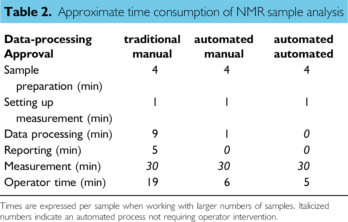
Times are expressed per sample when working with larger numbers of samples. Italicized numbers indicate an automated process not requiring operator intervention.
Automated Approval
To further reduce operator workload, the approval process can also be automated. There is some further time to be gained as can be seen in Table 2. The benefit will be more pronounced when samples are processed individually or in a smaller series due to the overhead of logging in on the computer, starting up programs, navigating folders, etc. By automating the approval process, analytical results will automatically become available to the requestor when samples have been measured.
Evaluating whether a spectrum is similar to the reference in terms of peak shape and peak position is something that a computer can easily do on the basis of the statistics, as discussed previously. Besides, a sanity check can be incorporated that judges whether the actual results make sense flagging samples with compositions that are physically impossible, for example, where there are excessive end-group concentrations relative to repeat units.
A particular family of copolymers that needed to be analyzed frequently consisted of three different monomer repeat units. The results from the NMR spectrum were the percentages of each of these repeat units (three data points), nine different end groups (combinations of functionality and terminal monomer unit), and two more moieties formed by side reactions. In addition to these 14 data points for these samples, the automated processing collects 15 values that quantify spectral shifts to match peaks to the reference spectrum, 15 correlation coefficients that describe the peak similarities with the reference spectrum, and 15 integral fractions that quantify the fraction of area in a particular snippet of the spectrum that falls in between the predefined integration limits. For each of these 45 processing parameters, the average and the standard deviation were calculated in a sample set of 168 samples, which had been approved manually. Now, each individual sample was evaluated as follows. For every parameter that falls outside the range of the average plus or minus three times the standard deviation, the sample receives a penalty point. This way, a sample can receive up to 45 penalty points.
The distribution of penalty points for the 168 correctly processed samples is shown (in gray) in Figure 21. Most of these samples has less than five penalty points. A second distribution (in black) shows the penalty points in a set of 12 erroneous samples. These are analyses in which the device was not properly shimmed (producing broader, poorly resolved signals), in which the signal lock failed, producing a file with just noise and several spectra of polymers with a different type of backbone than intended for the specified subroutine and a proton spectrum of a chemical rather than a polymer. For these samples, 11–16 penalty points are counted.
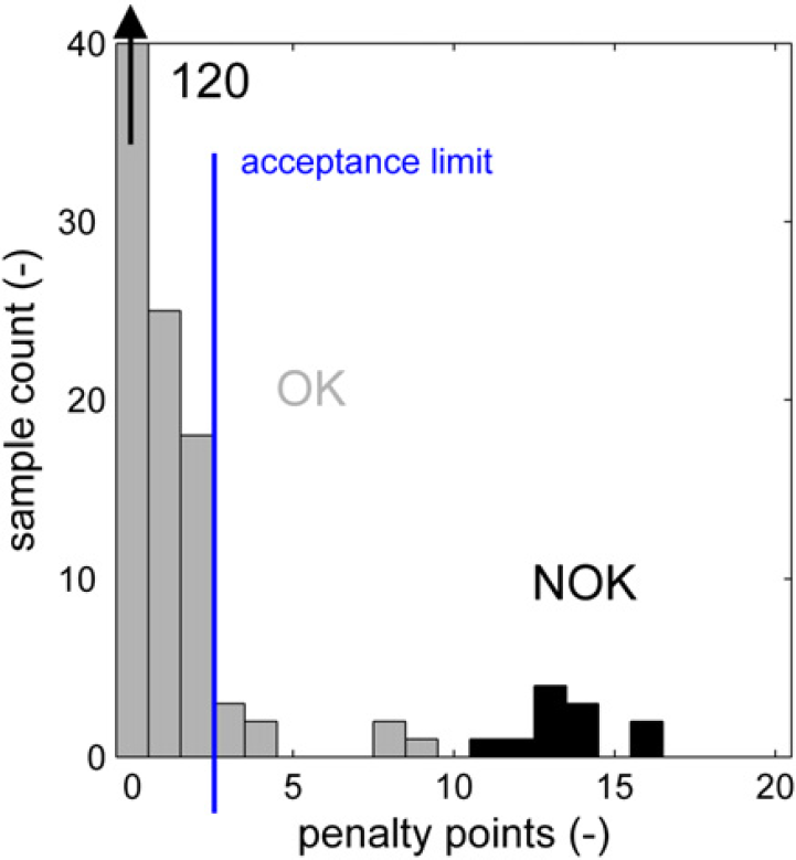
Penalty point distribution for good samples and erroneous analyses.
The autoapproval process should ideally approve all of the good (labeled “OK”) samples and not approve any of the erroneous results from incorrect samples or failed analyses (labeled “NOK”). This is indicated by the green areas in Figure 22. If correct results are not automatically approved, the process in Figure 3 follows the path from “autoapproval” to the “no action” end point and reverts to the manual approval process. This is not a worrying situation (orange area in Fig. 22), but it reduces the effectiveness of the autoapproval process if this is the case for a large portion of the samples. It is more important to prevent any incorrect results from being accepted by the approval process because this will lead to false entries in the laboratory database. This is the red area in Figure 22.
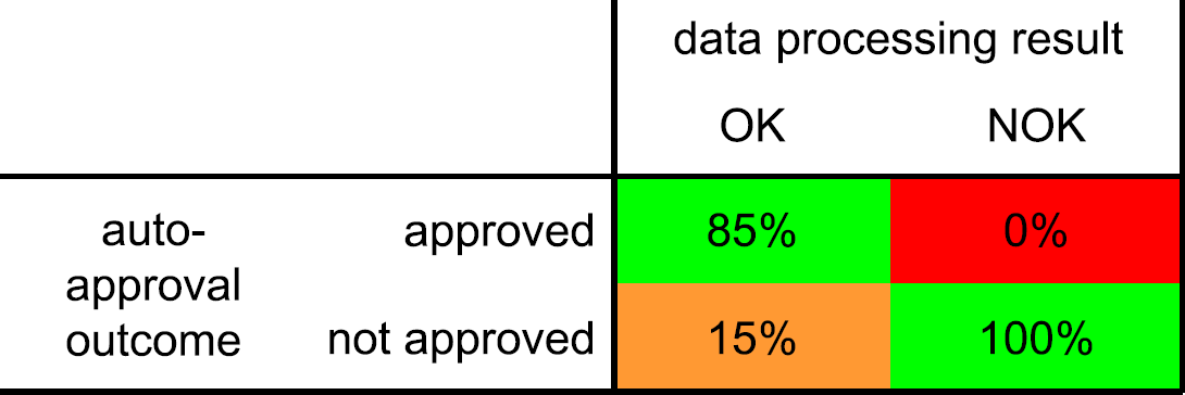
Approval matrix.
If the acceptance limit in the autoapproval routine is set at a maximum of two penalty points, and when the penalty points are considered to be distributed normally, the numbers in Figure 22 can be calculated. By setting the acceptance limit to the low value of two, it is assured that no incorrect results are evaluated as acceptable (a type II or β error in statistical terms). The 0% chance is better expressed using the finer grained unit of defects per million opportunities (DPMOs). Using this terminology, we arrive at the exceptionally low DPMO value of 14, which is extremely low.
Looking at the correct results, 85% is recognized as such and automatically uploaded into the laboratory database. The 15% correct results that have more than two penalty points are not uploaded and will need to be evaluated and approved manually.
Performance and Conclusions
By automating our semiroutine NMR analyses, we have been able to reach the desired level of NMR productivity to support the ongoing research and development projects. A reduction of handling time from 19 min down to 5 min per sample lead to a significant capacity increase. Part of this capacity was used for increasing productivity. The annual sample throughput doubled from 1400 to 2800 analyses during the first 2 years in operation. The remaining resources that were freed up were spent on nonroutine NMR spectroscopy, data interpretation, and method development, tasks more in line with the skills of experienced NMR personnel. While boosting productivity, quality also improved. This was expressed in a reduced number of questions around reported results. Turn around times reduced from about 6 days to less than 2 days for samples captured by the automation process. Around 80% of all NMR analyses were processed automatically.
Reflecting on the various types of muda that were identified in this process, we have shown that we have eliminated most of the motion, the nonvalue added moving around of results and data between applications. By automation, the sample is processed all the way through the end result eliminating waiting at the various steps of the previous workflow. The single-piece-flow approach allows all samples to be processed in a mode we used to reserve for urgent samples. When measurement is complete, processing and reporting is done straight away without any impact on efficiency.
We initially encountered a good deal of skepticism about automated NMR data processing. When experimental results were different from expectations, several analyses were manually verified to confirm the results and build confidence in the application. Eventually, the consistency of the automation lead to strong support for this approach. The inertness of the hardware and software to social pressure in the form of normative and informational influences to conform to certain expectations from the requester of the results proved to be an important asset. 10
The enhanced data consistency and uniformity in administration of the samples lead to fewer samples requiring rework after their first pass through the process and reporting of results.
Considering the scope of the project, not touching upon the NMR software nor the laboratory database itself we have successfully minimized the amount of human intervention that is required on routine samples while improving result quality.
In addition to our initial targets, the ability to process large sets of samples in an identical manner proved to be very valuable. It allowed us to identify unknown peaks by correlating them to known signals in the spectrum. Reprocessing spectra with calculations based on the newly identified peaks is rapid (< 10 s/sample) and is easily performed. After updating the appropriate integration routine, one only needs to remove the sample entries from the Excel spreadsheet software file list such that the samples are considered to be new by the automation software. After discovery of a specific degradation mechanism in a particular polymer backbone upon accelerated UV aging, the peak corresponding to the moiety that was generated in this process could be quantified in several hundred aged and unaged samples, which had been synthesized in over a year and which were analyzed before. This allowed a strong correlation between this degradation product and the material color stability based on an enormous data set within several hours.
We are very satisfied by the performance of the automated data processing that has resulted in a significant increase in productivity. Currently, we are looking to implement this approach globally within our company. With the automation framework in place, the resources needed to set it up at other NMR devices will be significantly smaller than the 0.8 f.t.e. needed for the first implementation in our laboratory in Bergen op Zoom.
Acknowledgments
The authors would like to thank Michiel Oudenhuijzen for his initial work on baseline correction and signal alignment in Matlab, Ben Jonker for his support on interfacing the LIMS database, and Han Vermeulen for supporting the implementation on the NMR workstation.
Competing Interests Statement: The authors certify that they have no relevant financial interests in this manuscript.
Footnotes
a
Microsoft, Excel, and Windows are either registered trademarks or trademarks of Microsoft Corporation in the United States and/or other countries.