
Abstract
A move from fixed, statically scheduled laboratory automation systems to more dynamic and adaptive behavior introduces complexities and challenges that have not been thoroughly explored in the field of laboratory automation. Powerful tools are required for the systematic modeling, analysis, simulation, and control of such systems. In this first part of a tutorial series, we introduce and explore Petri nets as a tool that can be used to model dynamically controlled laboratory automation systems. Subsequent contributions to this series will look at formal mathematical techniques for analyzing Petri net models, and methods for simulating and controlling laboratory automation systems using Petri nets.
Introduction
Static scheduling software is the tool used predominantly for planning the coordination and execution of integrated laboratory automation systems. Static schedulers lay out and arrange a sequence of instrument tasks on a timeline prior to execution. Sequences are assembled in an effort to optimize some aspect of procedure execution, such as the maximization of instrument utilization or sample throughput, while simultaneously ensuring that samples are processed in a desired manner and within specified performance constraints. Usually, a separate program will execute the tasks that have been placed on the timeline by the scheduler. Static schedulers have worked well for the processing of sample batches on many automated laboratory systems.
Unfortunately, unexpected events and sample characteristics can turn a highly optimized process into an inefficient one, resulting in a variety of undesirable outcomes such as excessive delays and ruined samples. For example, something as simple as a microplate being placed out of alignment or the failure to read a bar code on a sample container can cause a statically scheduled system to halt execution until an operator has intervened. More subtle problems can occur such as an unexpectedly slow rate of reaction or an unexpected precipitate. Nevertheless, many laboratory procedures require precise timing and strict adherence to protocols. In these cases, static schedulers have been invaluable tools for getting the most out of an integrated laboratory automation system.
When the execution details of an automated procedure are less strict and outcomes are not as well understood, an automated system may be much more successful if it can dynamically adapt to unanticipated events or unusual sample behavior. Such dynamic behavior can be very powerful and even bring new capabilities to integrated automation systems. For example, dynamically controlled systems can process each of its samples in unique ways, with multiple methods executing simultaneously on one system. The system controller can run continuously for extended periods of time; there is no requirement for the concept of a sample batch. With such a system, a scientist introduces one or more samples and assigns methods to each. The system executes all the methods, interweaving the tasks and dynamically prioritizing the utilization of system resources against other methods currently being executed by the system. Furthermore, sample methods can be modified on the fly, with the system adjusting execution details as necessary. Finally, new tasks can be added automatically based on the results of previous measurements while the system is running. When properly designed, the systems we describe can be thought of as evolving in a desirable manner, dynamically assigning resources and selecting tasks for execution rather than executing prespecified task sequences.
Unfortunately, dynamically controlled systems are themselves susceptible to many difficulties. For example, such systems can easily evolve into a state that prevents any further progress—a situation called deadlock. When deadlocked, a system cannot proceed due to the need for resources that will never become available. Consider the trivial scenario in which a robot is holding a microtiter plate, ready to place it into a plate reader, but cannot do so because there is a plate in the reader already. The robot would be required to remove the existing plate from the reader, which is not possible because it is already in the process of moving another plate to the reader. The system cannot proceed because the two resources that are required, the robot and the plate reader, are both being utilized and neither will become available. This scenario is a simple illustration of the kind of deadlock that can occur with dynamically controlled systems. In practice, more complex deadlocks can occur, involving many more than two resources. These deadlock situations can be hard to detect by simple inspection prior to execution.
The dynamic nature of such systems also can lead to situations in which a particular task is never executed due to competing task priorities or persistently unavailable resources. This is referred to as an unreachable state. Behavior such as this must be detected prior to execution and designed out of a system or avoided in order for the system to operate in a desirable manner.
Another problem that arises is buffer overruns. Nests, incubators, and other instruments that hold samples or movable labware can be thought of as buffers. The required capacity of buffers in dynamically controlled systems is hard to estimate for obvious reasons. It would be easy to design a system that was unnecessarily limited in its throughput due to low buffer capacities. Moreover, when buffers fill, they can be the cause of unexpected deadlocks. On the other hand, it would be wasteful to design systems with large and expensive incubators that can never be utilized because of other bottlenecks that go unrecognized until the system goes into production.
The throughput rate and task execution timing of dynamically controlled systems is hard to estimate, especially when multiple methods with nondeterministic task durations are executing simultaneously. More generally, the only realistic way to perform such an estimate is through the use of stochastic simulations. In these simulations, many scenarios are tested with parameter values and resource allocation choices sampled from statistical distributions. The result of such an analysis is a set of anticipated average performance metrics with an estimated variability.
Circumventing all of these problems requires the identification and application of a powerful tool for the modeling, analysis, simulation, and control of dynamic laboratory automation systems. For this purpose, we will introduce and investigate the application of a technique called Petri nets.
This manuscript is the first in a series of tutorials that will explore Petri net and their application to integrated laboratory automation systems. We introduce Petri nets and their extensions, and explore their use as a tool to model automated laboratory systems. In subsequent parts of this tutorial series, we will study methods for mathematically analyzing Petri nets to discover their properties, as well as methods for running Petri net simulations.
Background
Petri nets were introduced by Carl A. Petri in 1962, 1 and have been actively studied, applied, and enhanced ever since. Petri nets are a powerful graphical and mathematical tool for modeling, analyzing, and simulating a wide variety of systems. They are especially applicable to discrete event systems characterized by concurrently executing processes that are asynchronous, nondeterministic, and/or stochastic in nature. They have been applied in a wide variety of fields, from computer system hardware and software to workflow processes. 2 One area of particular interest to us is the application of Petri nets to flexible manufacturing systems, 3 due to the similarity between manufacturing and the field of laboratory automation.
Manufacturing systems take raw materials as input and process those materials in order to create a product. The manufacturing process is often broken down into steps, with each step being performed by an individual work cell. Materials are routed from work cell to work cell as they are turned into the final product.
Flexible manufacturing takes the process a step further. Flexibility comes from an ability to dynamically reroute materials to different work cells in order to achieve a variety of desirable outcomes: simultaneous manufacturing of different products, load balancing, avoidance of a malfunction, and more. Petri nets have been used for years to study manufacturing systems, especially flexible manufacturing.
The manner in which Petri net theory can be applied to laboratory automation systems follows naturally from a consideration of the similarities between laboratory automation and flexible manufacturing. Raw materials and manufactured products are like laboratory samples such as biological samples to be tested, compounds to be synthesized, or cell cultures to be grown. Manufacturing work cells are like laboratory instruments such as measurement devices, incubators, or synthesis reactors. Manufacturing processes are like laboratory procedures such as sample screening, compound synthesis, or cell culture growth. With these correspondences in mind, results from the extensive literature that applies Petri nets to manufacturing also can suggest ways in which Petri nets can be applied to laboratory automation. We have found that Petri nets can be very useful in helping to solve the difficulties that arise with dynamically controlled laboratory automation systems.
The graphical and mathematical nature of Petri nets lends itself nicely to support from a software tool. Many software tools and libraries have been developed over time. A database of Petri net tools is available from the University of Aarhus, Department of Computer Science, Denmark. 4 The available tools are too numerous to mention. Nevertheless, we call attention to a few that we have found useful. At least three Matlab 5 (The Math Works, Natick, MA) Petri net libraries are available. One is from the Department of Automatic Control and Industrial Informatics of the Technical University “Gh. Asachi” of Iasi, Romania, 6 and another is available from the Center for Applied Cybernetics, Czech Technical University in Prague 7 . A third, from the University of Notre Dame (Notre Dame, IN), focuses specifically on the supervisory control of Petri nets. 8 A popular tool for a special kind of high-level Petri net called Colored Petri nets 9 is available from the CPN Group, University of Aarhus, Denmark 10 . A tool written in the Java programming language 11 called the Petri Net Kernel for Petri net simulation is available from the Humboldt University, Department of Computer Science in Berlin 12 . One final tool that is worth mentioning is the Platform Independent Petri net Editor (PIPE2), which is being developed at the Imperial College, London. 13 It is written in Java, and provides a nice graphical designer with sophisticated analysis and basic stochastic simulation capabilities.
Models
In this section we define the main components of a Petri net as well as rules for execution, and introduce the basics of building Petri net models.
Elements
As mentioned previously, a Petri net is both a graphical and a mathematical tool. From a graphical perspective, a Petri net is a special kind of graph composed of two node types: places and transitions (Fig. 1). Places are depicted as circles, and transitions as straight lines or bars. Arcs are used to connect places and transitions. The resulting graph is a Petri net. Nodes of the same type are never connected directly by an arc. Places can be directly connected only to transitions, and transitions only to places. It is also possible for two nodes in a Petri net to be connected with multiple arcs. This is often represented in a diagram by weighting a single arc with an integral value equal to the number of arcs that connect the two nodes rather than drawing multiple arcs. In a formal graph theoretic sense, Petri nets are bipartite directed multigraphs.
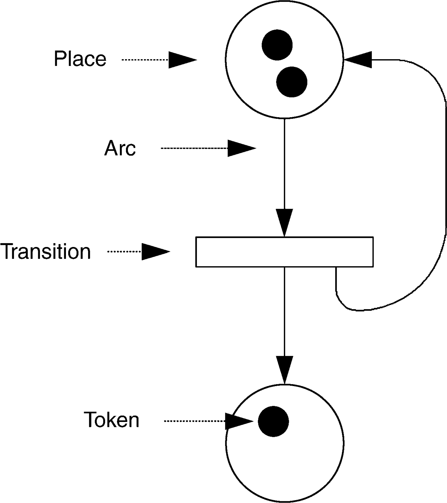
A simple Petri net.
If a place is connected to a transition with an arc that leads from the place to the transition, the place is referred to as an input place of the transition. An output place of a transition is a place connected to the transition with an arc that leads from the transition to the place. An output place of one transition can be an input place of another transition. Input transitions and output transitions are defined in a similar manner with respect to a place.
Places and transitions can contain zero, or more circular symbols called tokens. During the execution of a Petri net, tokens can travel from node to node along the directed arcs that connect them. Transitions consume tokens that flow in, and create tokens that flow out. The distribution of tokens over the nodes of a Petri net is called a marking, and represents the current state of the Petri net. The very first marking of a Petri net, prior to execution, is called the initial marking.
Governing Rules
Two rules govern the execution of a Petri net. The enabling rule determines if and when a transition is enabled. The firing rule determines how tokens are removed from input places and added to output places.
Transitions are enabled if and only if each of its input places contains at least one token for every arc that connects the input place to the transition. This is called the enabling rule. When a transition is enabled, it may fire. A firing transition removes a number of tokens from each input place (one token for each incoming arc) and places one or more tokens in each output place (one token for every outgoing arc). This is called the firing rule. Together, the enabling rule and firing rule are used to evolve the state of a Petri net. This process is called the token game.
On its own, the firing rule is not conservative. In other words, the number of tokens consumed during the firing of a transition may not equal the number of tokens created. For example, if a transition has two incoming arcs and one outgoing arc, when the transition fires, two tokens will be removed from its input places, but only one will be added to its output place. In a subsequent part of this tutorial series, we introduce a well-known algorithm for determining the subnets of a particular Petri net that do conserve tokens, as well as the conservation rules that describe them when they exist. 14 In this situation, the total sum of all tokens on the subnet does not change as the Petri net executes. Token conservation is an important property when applying Petri nets to problems in laboratory automation. Fortunately, this algorithm is built into several available Petri net software tools.
If two transitions are enabled by tokens in a shared input place, but the input place has an insufficient number of tokens for both transitions to fire, the network is said to be in conflict. For example, consider Figure 2. Both transitions are enabled, but only one can fire because there is exactly one token in p1, the shared input place. It would be necessary for p1 to contain two tokens for both enabled transitions to fire. Deciding which to fire is outside the scope of the Petri net's execution, and is often determined by an external control system or prioritization scheme.
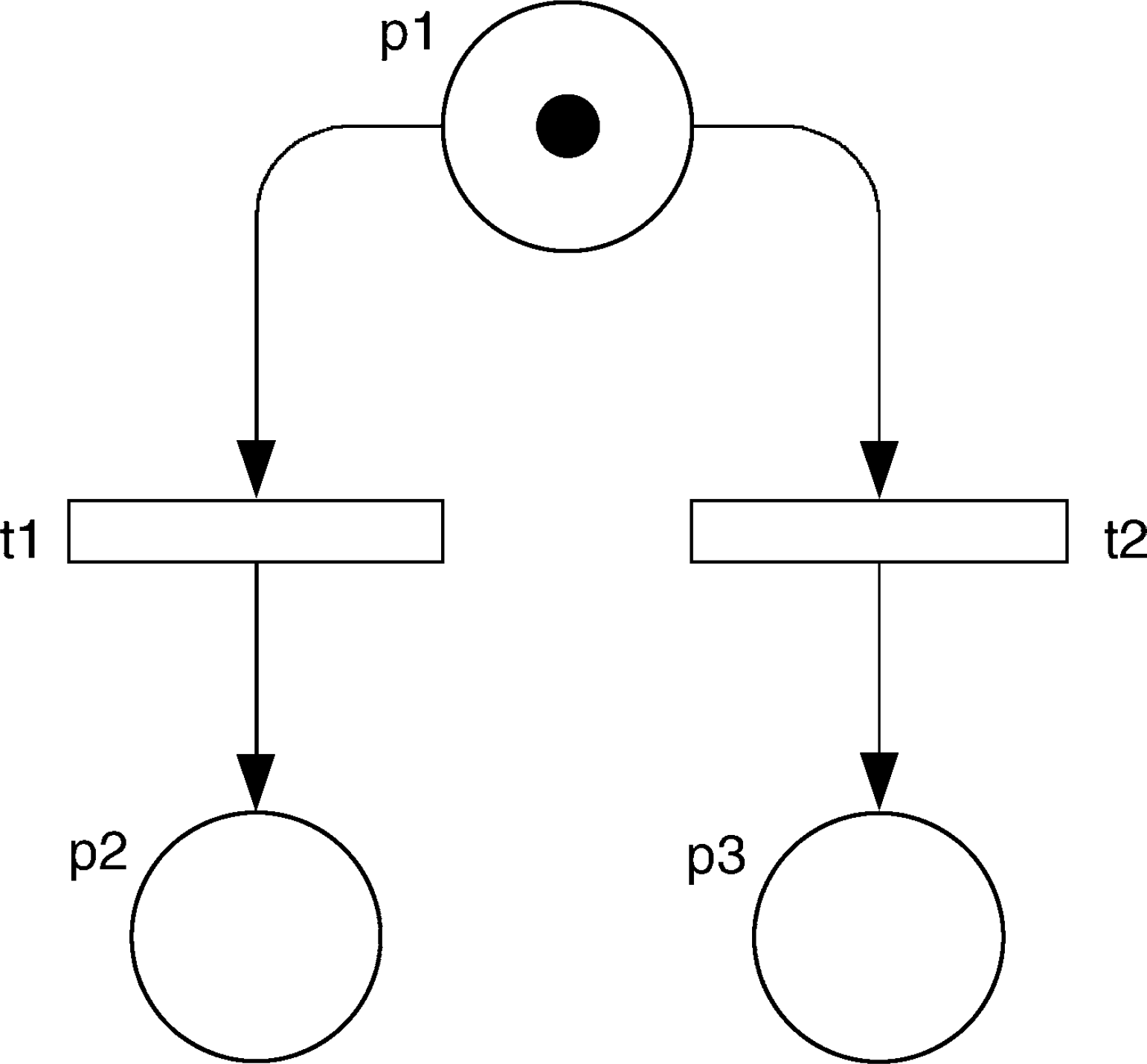
A Petri net in conflict.
Interpretations
The elements of a Petri net have no intrinsic meaning. It is up to the modeler to assign a meaning that is appropriate to the model. There are several common ways to interpret the meaning of the places and transitions of a Petri net. We will discuss these in the context of automated laboratory systems.
A place is often used to represent the availability of limited resources. When a resource place contains a token, the meaning implied is that the resource is available for use. The existence of multiple tokens in a resource place implies that multiple resources are available. For example, assume we have a place called Reader 1 Available that contains one token (see Fig. 3). This can be interpreted as meaning that the reader resource is available to perform an action. After firing a transition that consumes the token in the Reader Available place, the reader resource has become busy (is no longer available). Only after a token is moved back into the Reader 1 Available place will the reader once again be available. The same argument applies to plate p9, Reader 2 Available.
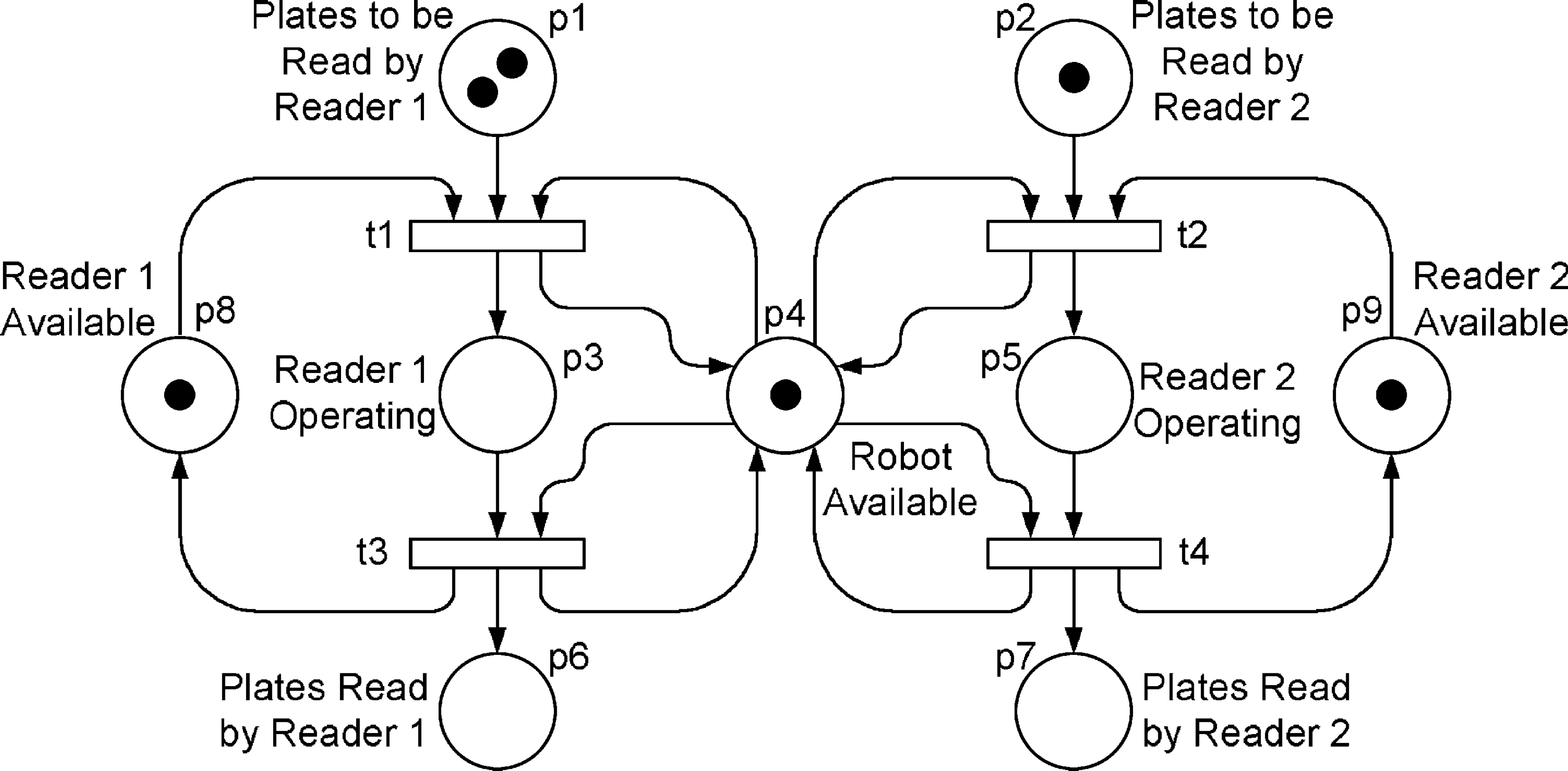
A simple Petri net with place interpretations.
Places can also be interpreted as a type of buffer. In Figure 3, places p1 and p2 are input buffers that contain tokens representing plates to be read by Readers 1 and 2, respectively. Places p6 and p7 are output buffers that hold plates after they have been read. Transitions t1 and t2 become enabled if there is a token representing plates in each of the input buffers, and if the robot and corresponding reader are available. Because there is one robot resource (represented by a single token in place p4), only one of transitions t1 and t2 can fire at any moment in time. When t1 or t2 fires, in addition to removing a token from p4, a token is also removed from the place that corresponds to the input plate buffer and associated reader.
A third common interpretation of a place is as a condition. If a condition place contains a token, the condition is said to be satisfied. If the place is empty, the condition is not satisfied. For example, a token contained within a specific place may be interpreted as an indication that a reactor has reached or exceeded a predefined temperature set point. The lack of a token would indicate that the temperature is below the set point value.
Another commonplace interpretation is as an activity. When an activity place contains a token, the implication is that the represented activity is currently being performed. Places p3 and p5 in Figure 3 represent reader operation activities for plate readers 1 and 2, respectively. When one of these places contains a token, the corresponding Reader Available place is missing its token and the plate reader is considered to be operating. When the output transition of one of these activity places is fired, a token is removed from the input activity place and a token is placed in both the corresponding output buffer places and back into places p4, the Robot Available place, and the associated Reader Available place. At this point the plate reader is considered to have stopped operating and is available for other tasks.
Transitions can also have multiple interpretations. A common interpretation for a transition is as an event. In this case, a firing transition models the occurrence of an associated event. For example, a transition may represent the moment when the temperature of a reactor reaches its set point. The event is modeled by the firing of the transition, which can add a token to a place that indicates that the minimum temperature condition has been reached.
Up to this point we have assumed that when a transition fires, it does so instantaneously. There is no duration associated with the firing of a transition in a simple Petri net. If we relax this assumption, we can allow a transition to fire over a finite amount of time and to hold on to tokens that it removes from input places while it is firing. Only upon the completion of firing will tokens be added to the transition's output places. In this scenario, we can interpret the firing of a transition as modeling the execution of an activity. For example, in Figure 3 the firing of transition t1 can be interpreted as the execution of an activity during which time the robot picks up a plate from the first input buffer and places it in the first plate reader. We will look further at transitions as activities in the next section.
Extensions
A basic Petri net, as defined by its elements along with the enabling and firing rules, is a powerful formalism. Nevertheless, to apply the tool to more realistic situations, especially those in the field of laboratory automation, three common extensions are employed. 15
Time
As tokens are manipulated by the elements of a Petri net, they can be required to remain within an element for an amount of time that is either predetermined or sampled from a statistical distribution. A Petri net with an extension such as this is referred to as a timed net (when fixed time durations are used) or a stochastic net (when time durations are drawn from probability distributions). The addition of timing is necessary if Petri nets are to be used to analyze properties such as system performance, cycle time, or scheduling behavior.
We have already introduced the idea of assigning a firing time duration to the execution of a transition. The concept of time also can be imposed upon places by adding a time stamp property to each token. The time stamp indicates the time after which the token can be used to enable an output transition. During the period prior to the value of a token's time stamp, a transition must rely upon other tokens to become enabled. The token's time stamp value would be set as part of the execution of a Petri net.
Color
A second and very compelling extension to Petri nets is the so-called extension with color. 9 A colored Petri net is so named because its tokens are said to be colored in such a way that indicates token type information. Stated in another way, colored Petri nets use tokens that can hold data values. The time stamp of tokens in a timed Petri net can be thought of as one example of such a data value. If tokens can have associated data values, one can begin to think of tokens as modeling real objects. For example, the token in p4 of Figure 3 (the Robot Available place) can be thought of as the robot itself. Tokens in p1 or p2 (one of the Plates to be Read places) in the same Petri net can be thought of as plates. Tokens in p8 and p9 (the Reader Available places) can be thought of as plate readers. Firing of transition t1 would not consume these tokens, but rather would combine the data from each input token into one composite token when transferred to p3 (the Reader 1 Operating place). After a plate is read, the output transition would reconstruct the robot token, reader token, and plate token, and route them to their appropriate output places.
The addition of data to tokens opens the way to label arcs with guard conditions, which is another characteristic of colored Petri nets. In addition to the enabling rule, to fire a transition in a colored Petri net, the guard condition that labels each incoming arc of a transition must also be satisfied by the data of one of the tokens in the connected input place. Only if a token can be found that satisfies the guard condition will the transition fire. While firing, a transition may also execute a function that modifies data in the tokens being manipulated. As an example, we merge the input buffers of Figure 3 into a new place called p1-2 and label each plate token with a number indicating its type. The new Petri net is depicted in Figure 4.
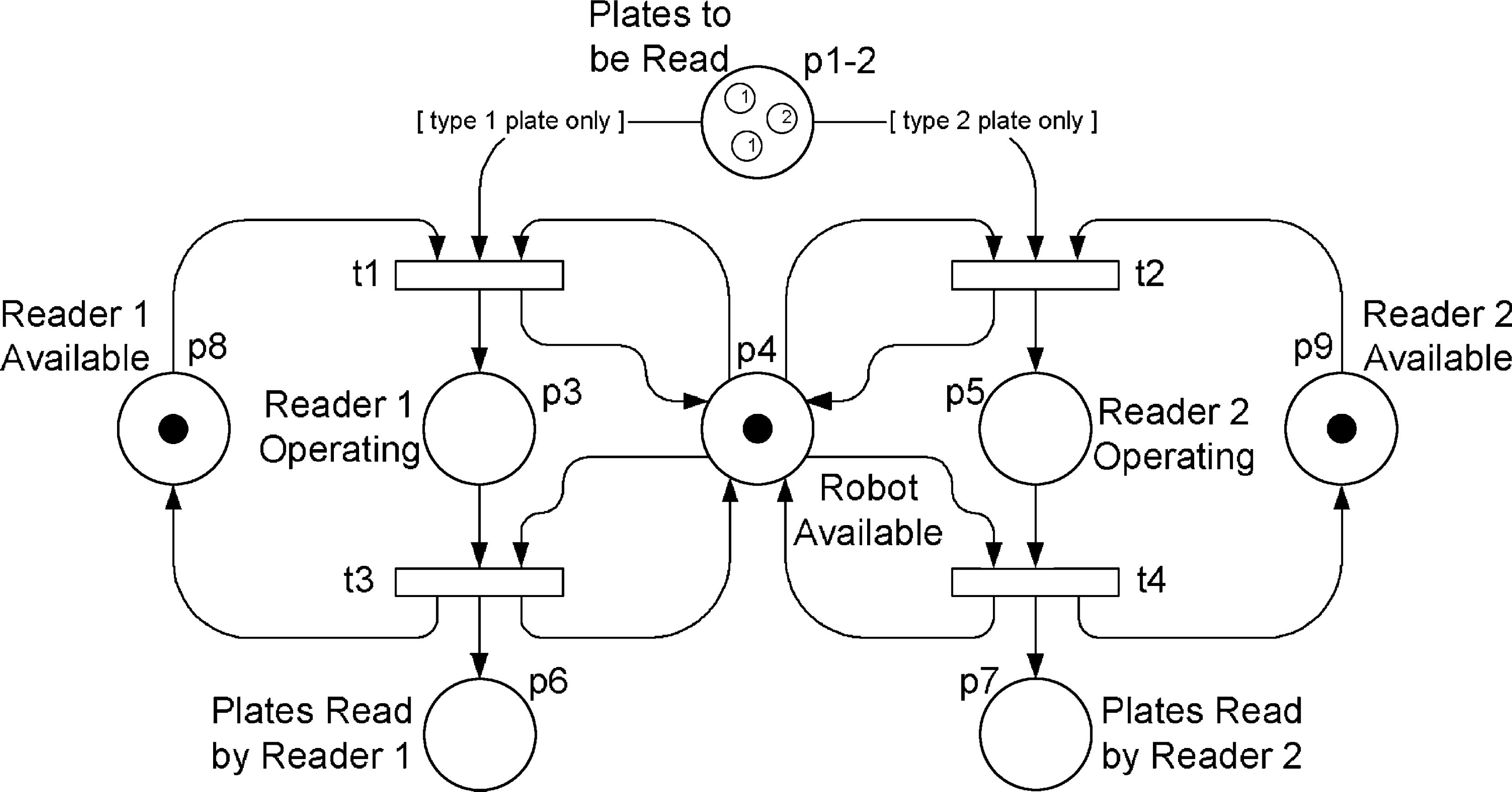
A colored Petri net with guard conditions.
Also note that we added guard conditions to the arcs connecting the input buffer to one of the two transitions leading to a plate reading operation. The guard conditions are contained within square brackets and act as a filter on plate tokens that can be routed along an arc. Plates routed to Reader 1 must be of type 1, and those that are to be routed to Reader 2 must be of type 2. This is possible only because plate tokens are labeled with data that indicate their type.
Hierarchy
A final Petri net extension is that of hierarchy. Models of real world problems tend to generate large and complex Petri nets. These Petri net models quickly become unwieldy due to their size. In a Petri net extended with hierarchy, a transition or place may itself represent an entire subordinate Petri net. A firing transition in a hierarchical Petri net may be governed by the execution of a self-contained subordinate Petri net. As the subordinate Petri net completes execution, the transition in the higher Petri net completes its firing process. Similarly, a single place in higher level Petri nets may also represent a complete subordinate Petri net. In this case the subordinate net must have a single start place and a single end place. A token entering the place in the higher level Petri net is equivalent to the token entering the start place of the subordinate net. When the token reaches the end place of the subordinate net, it becomes available in the higher level net to enable outgoing transitions.
Examples
In spite of the apparent simplicity of Petri nets, the systems that can be modeled are diverse, displaying significant breadth and complexity. Several examples are explored in the following sections to illustrate how one can use Petri nets to model more complex laboratory automation systems. These represent only a small sampling; a comprehensive collection of models is well beyond the scope of this tutorial. Fortunately, the similarity between manufacturing and laboratory automation makes it a straightforward task to translate easily from one domain to the other. An extensive treatment of the application of Petri nets to manufacturing is available. 3
Sample Processing
Many styles of sample processing can be modeled using Petri nets. The simplest, the sequential execution of a series of tasks, is modeled as a Petri net made up of nothing more than a connected series of alternating places and transitions. The central vertical path through the Petri net of Figure 5 is an example. Resources are easily added to the model using resource places and an appropriate number of tokens. The robot (p7), dispenser (p5), and reader (p6) resources represent the added resource places in Figure 5.
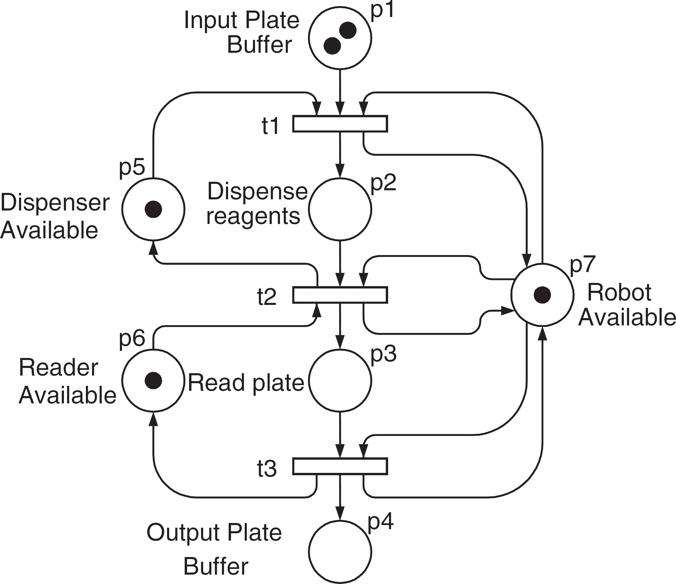
Sequential tasks with resources.
Modeling the parallel processing of samples is natural using the Petri net formalism. We've already seen examples of this in Figure 3 and Figure 4. Two readers can process plates simultaneously.
The splitting of a single workstream is accomplished with the addition of multiple output arcs leaving a transition. Rendezvous, a complementary operation requiring that multiple parallel streams complete prior to moving ahead, is modeled with multiple incoming arcs to a transition. Tokens must be present in all input places before the transition will fire.
A situation in which resources are limited resources is handled by ensuring that only one token per available resource is added to a resource place. The single token in p5 of Figure 5 indicates that only one dispenser resource is available.
Transportation Systems
A commonly used tool for transporting samples in automated laboratory systems is the robotic arm. Irrespective of the style (Cartesian, cylindrical, or other), robotic arms used in laboratory automation tend to be random access devices; they are designed to move samples from any point to any other point within an integrated system. In this sense, there tends to be no practical restriction on the use of robots, and as a result, they can be treated as simple resources and modeled using a resource place containing one token for each robot in the system. The Robot Available place in Figure 3 and Figure 4 is an example of this. When a robot is busy transporting samples, a robot token is removed from the resource place. When a robot becomes idle and is available for other tasks, a token is placed back into the resource place.
Another class of sample transport device that has been used for some time in clinical testing laboratories, and has also become increasingly popular in BioPharma laboratories over the past several years, is the linear sample conveyor. In automated clinical testing laboratories, a typical sample conveyor transports tubes along a track and directs them to appropriate sample processing workstations. Clinical testing laboratories can have hundreds of feet of tube conveyor track with many side branches.
Linear conveyors in BioPharma laboratories typically take a different form, but perform the same essential function. Conveyors such as the Thermo (Thermo Electron Corporation, Burlington, Canada) CRS High Speed Distributed Motion System 16,17 transports microplates to various locations within a system using a high-speed conveyor belt. Small robotic devices called Flip Movers, stationed along the length of the belt, exchange microplates between the belt and plate processing equipment.
A variation on this idea is embodied in Caliper Life Science's Allegro Systems (Caliper Life Sciences, Hopkinton, MA) which transport microplates along a linear series of workstations. Each workstation has its own dedicated robot responsible for moving plates into and out of the workstation's instrument, as well as handing off microplates to a workstation on either side. The result is a bucket-brigade style conveyor transport of microplates along the linear series of workstations. 18,19 Adjacent workstations share a single microplate nest (buffer). Workstation robots exchange plates, placing them into or retrieving them from shared nests.
Figure 6 is a Petri net model of a single Allegro workstation. The places in the four corners of the diagram represent the two buffers on either side of the workstation. These places are named Input Buffer Occupied (p1), Input Buffer Available (p2), Output Buffer Occupied (p3), and Output Buffer Available (p4). A token in p1 implies that there is a microplate waiting to be processed. A token in p2 implies that the input buffer is empty, and the adjacent robot is free to move a plate into the input buffer of the workstation to await processing. The case is analogous for places p3 and p4 representing the output buffer.
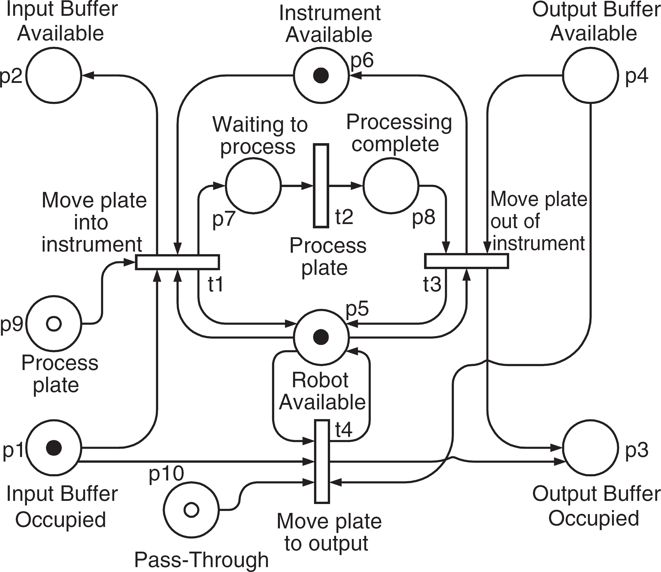
Petri net model of an Allegro Workstation.
Transition t1 (Move plate into instrument) will fire when there are tokens in p1 (the input buffer is occupied), p5 (the robot is available), p6 (the workstation instrument is available), and p9. Place p9 is a special kind of place called a control place. A token is placed in p9 by an external control system when the associated transition is allowed to fire. This is an example of how an external control system can guide the behavior of a Petri net. Control places are used to trigger or prevent actions.
After t1 is fired, a token is placed in p7 (Waiting to process), which will trigger transition t2 (Process plate). Upon completing plate processing a token will be deposited into p8 (Processing complete) where it will wait for the robot and output buffer to become available. When t3 fires (Move plate out of instrument), the output buffer becomes occupied, and the instrument is available for processing another plate.
If there is a token in places p1 (Input Buffer Occupied), p5 (Robot Available), and p4 (Output Buffer Available), and if the control system deposits a token in the control place p10 (Pass-Through), the robot will move the plate from the input buffer directly to the output buffer, bypassing instrument processing. Note that if both control places p9 and p10 contain tokens, then transitions t1 and t4 can both be enabled, and therefore they will be in conflict. The external control system must ensure that this situation does not occur; alternatively the Petri net can be designed to avoid the conflict. This is something that we will explore further in a subsequent part of this tutorial series.
A model of several Allegro workstations is constructed easily by recognizing that the output buffer of one workstation is the input buffer of the next. Figure 7 is a model of three Allegro workstations in series. The part of Figure 7 modeling the second workstation is drawn using dashed lines so that it can be distinguished from the first and third workstations.

A combined model of three Allegro Workstations in series. Workstation 2 is drawn with dashed lines.
Storage
A common form of sample storage in integrated laboratory systems is of the random access type. Examples include a tube rack, plate hotel, and actuated carousel, because these devices allow any sample to be accessed at any time. Random access storage in a Petri net can be modeled in a manner as simple as a single place that holds multiple tokens. As we have seen in Figure 6, limited storage can be modeled using two places, one place represents the available storage locations, and the other the storage locations that are occupied. The first place starts with a number of tokens that corresponds with the number of available storage locations. As storage locations are occupied, tokens are moved to the second place. When storage is full, no tokens remain in the place representing available locations. In the Allegro Workstations of Figure 6, the input and output buffers represent a single location storage device. When a token is moved from a Buffer Available to a Buffer Occupied place, the maximum storage is reached, and no further plates can be moved into the buffer. If we modify the location buffer that sits between two Allegro workstations, and change it from a single nest to a multilocation hotel, the only modification we would have to make to the Petri net model would be to add more tokens to the Buffer Available places. Of course, because our model permits only one plate at a time to be processed by the instrument, such a modification would have limited impact.
Another common storage device used in integrated laboratory automation systems is the plate stacker, a vertical plate storage device. Examples are the plate storage devices used by the PerkinElmer PlateTrak Robotic Liquid Handling System 20 and the Tomtec Quadra3 (Tomtec, Hamden, CT) 21 . Plate stackers are a kind of last-in first-out (LIFO) queue. Plates are pushed on the stack and removed off the stack using a device that is mounted below the vertical stack. Due to the way in which a plate stacker operates, the last plate pushed onto the bottom of the stack is the first plate that is removed from the stack.
Figure 8 is a Petri net model of a four-position plate stacker. Plates are added to the stacker through place p1 and removed through p12. Plates are stored in places p7 through p10. The initial marking of the net has a single token in place p2.
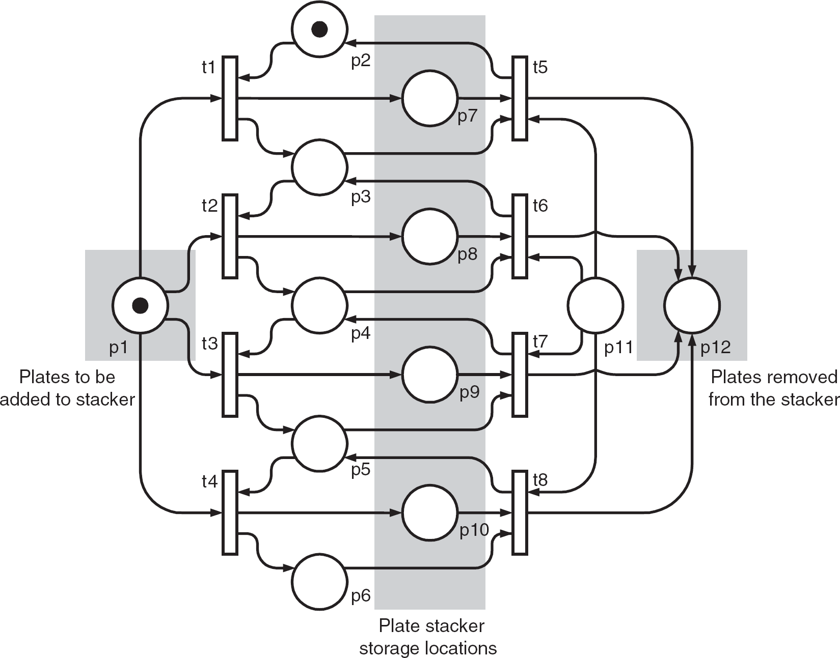
Petri net model of a four-position plate stacker (LIFO queue).
When the stacker is empty (a token is in place p2) and a token representing a plate is placed in p1, only transition t1 is enabled. When t1 fires, the token is removed from p1 and a token is added to p7, which is the first storage location of the stacker. Also, the token in p2 is removed and one is added to p3. When another plate token is added to p1, t1 cannot be enabled because p2 no longer contains a token. Transition t2 will be enabled because of the token that is now in p3. Firing t3 will remove the plate token in p1 and put a token in p8, the second storage location. Also, the token on p3 is removed and a token is added to p4. This process will continue until all storage locations are filled. Note how p7 through p10 are filled in order.
To remove a token from the plate stacker model, a control token is added to p11. If the stacker is full, the tokens in p6, p10, and p11 will enable transition t8. Transitions t5, t6, and t7 cannot be enabled because there will be no tokens in places p3, p4, and p5. When t8 fires, the plate token on p10 will be removed and a token will be added to the output place p12. Also, the token will be removed from p6 and a token added to p5. A second control token added to p11 will result in t7 being activated. When t7 fires, the plate token in place p9 will be removed, and a token will be added to the output place p12. Also, the token in p5 will be removed and a token will be added to p4. This continues until all plate tokens are removed from the stacker, leaving a token in p2-the state of the model when the stacker is empty. Note that the model captures the fact that plates are removed from the stacker in an order opposite to the order in which they were added. This is a LIFO queue.
Conclusion
In spite of the simplicity with which they are defined, Petri nets are a powerful graphical and mathematical formalism that can be used to model diverse integrated laboratory automation systems. A move away from statically scheduled integrated systems to more dynamically controlled and adaptive systems requires a powerful modeling, analysis, simulation, and controller development tool. Petri nets can fill this requirement.
In the following contributions to this tutorial series we will explore methods to analyze Petri net models of laboratory automation systems. It is our opinion that the real power of Petri nets is obtained when the model is reduced to a mathematical statement and analytical algorithms are applied to the model to discover its properties. We will conclude the tutorial series with a look at running simulations of Petri nets to discover additional properties and investigate behavior when analytical analysis becomes too complex.