Economic Justification of Laboratory Automation

Introduction

In these times of tight pharma R&D budgets, tightening academic budgets, and increasing merger and acquisition pressures (and following the burst of the biotechnology bubble), investments in laboratory automation demand justification beyond simple declarations that something is better or faster. Choices need to be analyzed to convince not only top management but also convince us that automation makes sense for an organization, be it an established pharmaceutical company, start-up biotech, or academic research center. Formal techniques exist to help complete this analysis and answer the key question posed by economic justification: Is this the best choice for an organization given limited funds?

Laboratory automation is a technological endeavor. As such, existing economic tools and financial techniques can be used to compare technology and investments based on economic measures of effectiveness. These tools and techniques are often called economic analysis, engineering economy, or economic decision analysis. ^{1 –3} Traditionally used in engineering and manufacturing, these techniques have become ingrained into public sector decision making and therefore are taught widely. They run the gamut from a simple comparison of alternatives to defining the return on investment (ROI), cost-to-benefit ratios, breakeven analysis, and more. Luckily, a comparison of alternatives for laboratory operations needs only a subset of these methods. In this JALA Tutorial, we present a primer on the basics of engineering economic analysis and describe several common methods for justifying the introduction of automation into a laboratory using plenty of examples.

The Present Economy Study

When judging alternatives, money follows one of two time frames: present economy or the time value of money. The easier of these two to understand is the present economy study, which ignores the way that the value of money changes with time. A present economy study is acceptable if one of the following criteria is met:

1. There is no investment of capital, only out-of-pocket costs.

2. After any first (capital) cost is paid, the long-term costs will be the same or proportional to the first cost, no matter which alternative is picked.

3. The alternatives will have essentially identical results regardless of the capital investment.

These conditions allow the person comparing alternatives to view the choice as occurring only once and only right now.

Example 1

A lab needs to purchase extra nitrile gloves as a one-time event, and it has a choice between two suppliers. Both provide the same number of gloves per box, with the same specifications. This is a one-time purchase (i.e., not part of a standing order); there will be no costs at a future time associated with the various economic alternatives, and it is not a capital expense (meeting criterion 1 above). Therefore, only the price in the present economy is important. If one supplier's product is $7 and the other's is $9, then the most economically effective choice is the $7 purchase.

Of course, this example is simplistic. More complexity can be added by taking into account quality issues or unquantifiable issues such as look and feel. Present economy studies come into use when various choices of equally capable equipment have different purchase prices but the same maintenance, support and consumable costs, and the same user acceptance. The purchase price at that time is the only factor needed to determine economic effectiveness.

Costs Terminology

Before looking at more realistic justifications involving the time value of money, we must define the types of costs (and income) that need attention as part of an examination of alternative solutions. These can be called the life cycle costs, which refer to all of the expenditures involved in a project or purchase throughout its entire useful life. For example:

• First cost: The total initial investment required getting an item or project ready for service, usually non-recurring, including purchase price, installation, modifications to infrastructure, etc.

• Operating and maintenance costs: Recurring costs necessary to keep the item in service, including service contracts and personnel salaries. These can be very large. These are also examples of future costs because they occur in the future.

• Opportunity costs: The costs of missed opportunities due to investing in the project in question. For example, when manual labor is not available for other projects, it can create a missed opportunity, and there can be a cost associated with that loss.

• Salvage value (income): Any money that potentially can be recovered for an item at the end of its life cycle. It equals market value less disposal costs. This can be especially difficult to calculate for laboratory automation.

• Product sales (income): If a product is being produced for sale, the projected income from each unit/dose/test sold can be used to offset costs. In this situation, the costs listed here should result in a profit.

Some of these costs are fixed costs, meaning that they do not change with the number of experiments, procedures, or operations performed, such as the purchase price. Otherwise, they would be variable costs, as they do scale with the amount of work performed, such as reagents consumed. All of the costs mentioned here are direct costs, meaning they are directly involved with the process in question, either as equipment, people, or material (including consumables and reagents). Indirect costs would be the costs of the building, utilities, upper management, etc. In traditional uses of economic analysis, these costs are used to help compare alternatives regarding where to locate a manufacturing plant, the infrastructure for that plant, and management organization alternatives. Very rarely does laboratory automation affect an organization to that level. Therefore, the focus of this tutorial is on the direct costs.

Time Value of Money

The value of money changes with time. It either gains worth over time if invested properly or decreases in value due to returns that are lower than the rate of inflation. Economic analyses consider this using the interest calculation. Following is an example of the mathematical relationships between the present and future values of money.

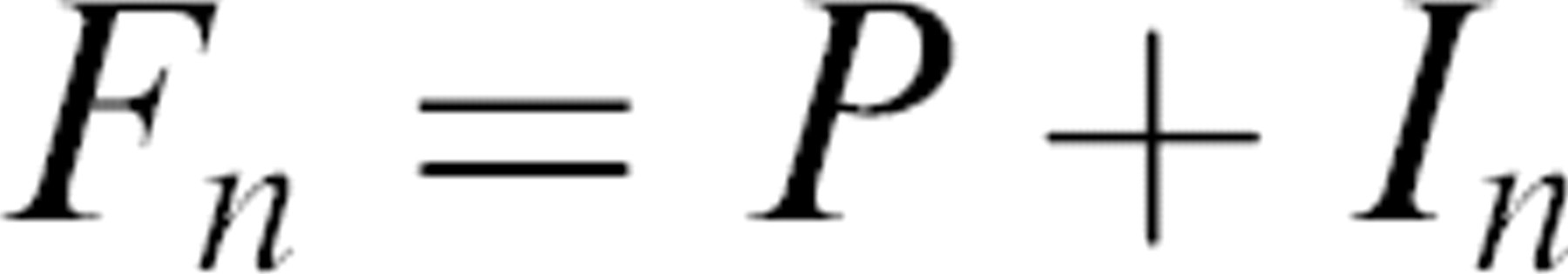
Let n be a number of years, and I_n the accumulated interest earned over n years. Then, the future value (F_n ) is related to the present value (P) by the equation

$F_n=P+I_n$

Now let i be the annual interest rate, which is the change in value of $1 over a 1-year period. There are two approaches to compute the value of I_n : simple and compound interest. With simple interest, P changes in value each year by an amount of P multiplied by i. In other words, for n years,

$I_n=Pin\hspace{1em}\text{and}\hspace{1em}{F}_n=P\left(1+in\right)$

Note, F is the future value of the money/investment and is almost never used in day-to-day personal life.

With compound interest, i is the rate of change in the accumulated value of money. In this case, F_n–1 is the future value of the previous year. This is the kind of interest with which most people are familiar:

$I_n=i{F}_{n-1}\hspace{1em}\text{and}\hspace{1em}{F}_n=F_{n-1}\left(1+i\right)$

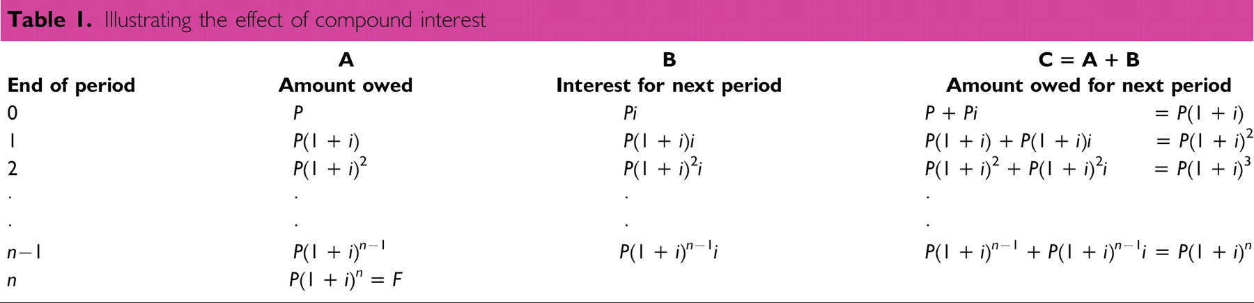
To judge the total effect of compound interest, we must create and summarize a table of the interest over a number of years. This relationship is shown in Table 1.

Single Sums of Money

The final equation from Table 1 can be used to find the future value of some present amount of money. A cash flow diagram can be used to describe this situation. This is a graphical representation of the flow of money into or out of an investment situation, shown on a timeline. Inflows are depicted as upward pointing arrows (income), and outflows as downward pointing arrows (cost or expense). Ideally, arrow lengths are proportional to the amount of money represented.

Table 1.

Illustrating the effect of compound interest

	A	B	C = A + B
End of period	Amount owed	Interest for next period	Amount owed for next period
0	P	Pi	p + Pi = P(1 + i)
1	P(1 + i)	P(1 + i)i	P(1 + i) + P(1 + i)i = P(1 + i)2
2	P(1 + i)2	P(1 + i)2 i	P(1 + i)2 + P(1 + i)2 i = P(1 + i)3
.	.	.	.
.	.	.	.
n–1	P(1 + i) n–1	P(1 + i) n–1 i	P(1 + i) n–1 + P(1 + i) n–1 i = P(1 + i) n
n	P(1 + i) n = F

Example 2

$40,000 (the present value, P) is invested into a 5-year certificate of deposit with 3% annual interest (i). The interest is reinvested and compounded once each year for 5 years (the number of interest periods, n). What amount of money will be available at the end of five years (the future value, F)?

Figure 1 illustrates the problem as a cash flow diagram. To solve this problem, use the equation F = P(1 + i) ⁿ. In standard economic analysis, this is written in a notation that is intended to be used with generated solution tables, which are provided with most economic analysis texts. For this problem, the notation is

$=P\left(F|Pi,n\right)$

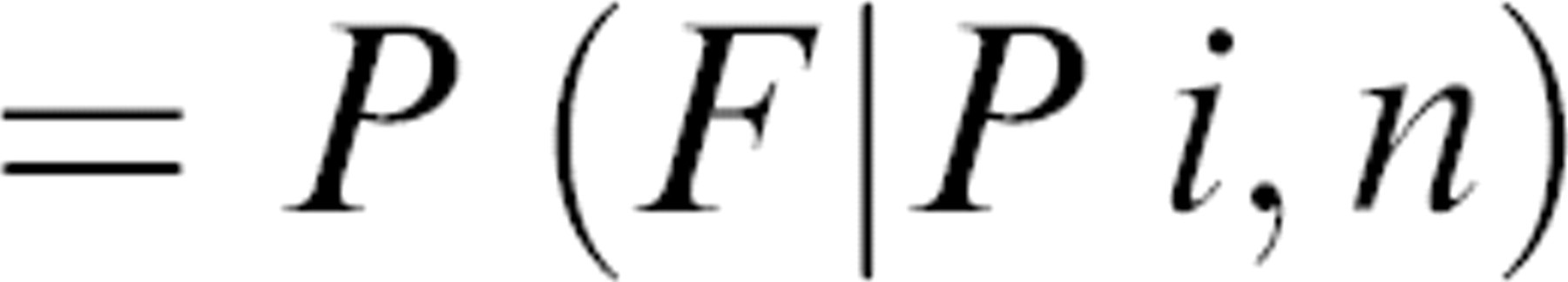
which is read as “the present value times the factor to find the future value given the present value, interest rate per period and number of interest periods.” Given the information from this example, the solution for the future value F is as follows:

${\begin{array}{c}F=\$40,000\left(F/P3,5\right)=\$40,000\left(1+0.03\right)\\ =\$40,000\left(1.159274\right)=\$46,370.96\end{array}}^5$

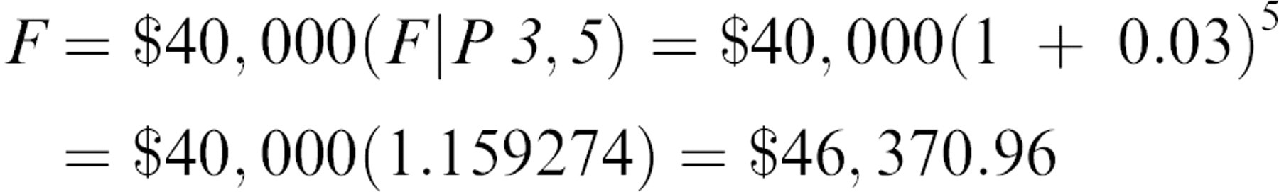
This yields an increase of $6,370.96 on the $40,000 investment.

This example illustrates a simple way to compare alternatives. Looking for the future value of multiple alternatives, even with different interest rates, allows the comparison of choices based on economic return.

Figure 1.

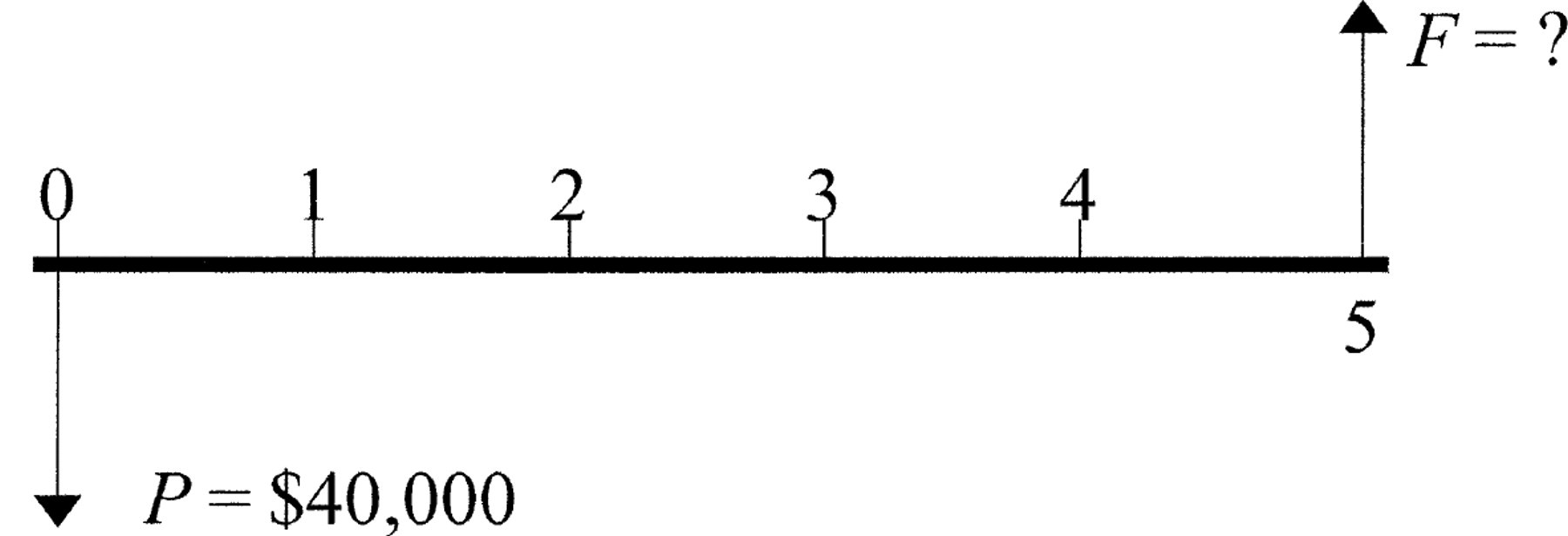
Cash flow diagram for example 2.

Series of Cash Flows

A more realistic technology investment situation involves multiple cash flows. Using present worth (also referred to as net present value), analysis means all cash flows will be converted to their present worth in order to assess the full economic impact of the project. This can be done via the following equation:

$P=F{\left(1+i\right)}^{-n}$

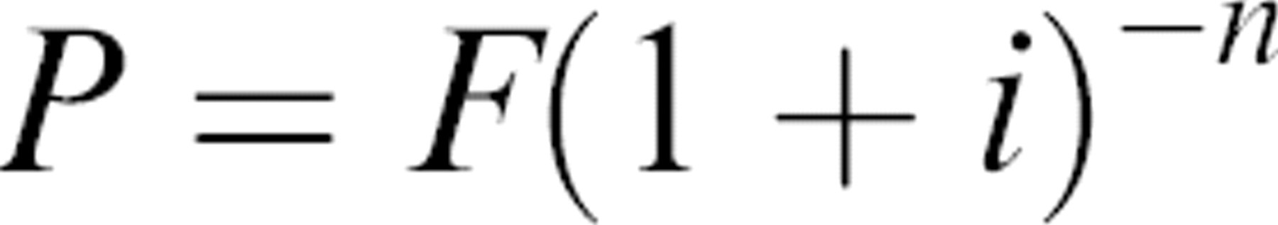
In standard economic analysis notation, this is written

$=F\left(P|Fi,n\right)$

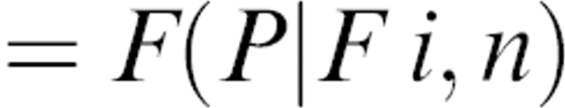
which is read as “the future value times the factor to find the present value given the future value, interest rate per period, and number of interest periods.” This yields the inverse of the previous equation, reducing a future cash flow by the change in value of the money over the number of interest periods to yield the true present worth.

Example 3

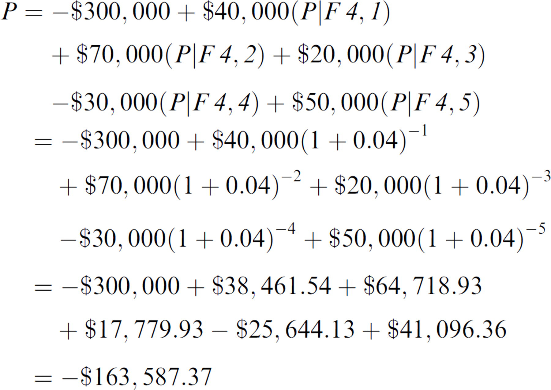
An off-the-shelf integrated automation system is purchased today for $300,000. It saves a company $40,000 next year, $70,000 the year after, and $20,000 at the end of the third year. In year four, it requires an overhaul of its components that costs $30,000. In year five, the company sells the system for a salvage value of $50,000 (see Fig. 2). Find the present worth of the entire series given an interest rate of 4% annually, compounded once per year.

Using the equation

$P\hspace{0.17em}=\hspace{0.17em}F\left(P|F\hspace{0.17em}i,\hspace{0.17em}n\right)\hspace{0.17em}=\hspace{0.17em}F{\left(1\hspace{0.17em}+\hspace{0.17em}i\right)}^{-n}$

we sum up all of the cash flows as follows:

$P=F(P|F\hspace{0.17em}i,n)=F{(1+i)}^{-n}$

Figure 2.

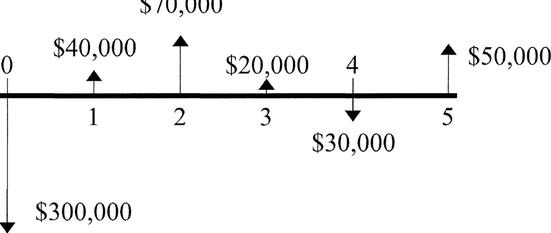
Cash flow diagram for description of example 3.

This result indicates that the technological investment costs $163,587.37 in today's money. Normally, to compare all of the possible alternatives for this task we consider costs at present worth and look for the least costly option (without taking into account other issues such as capital expenses, vendor pricing contracts, or tax deductions). Please note that different tables and calculators round differently. Some differences may appear, depending on where the factors are found or which calculator is used.

Uniform Series of Cash Flows

A uniform series of cash flows is a situation in which the same amount of money flows in or out over each interest period, either to return a future value or to pay back an initial investment. It can also be used to model consistent costs such as maintenance or labor. Another name for this type of series is the amortization series, which is used to determine monthly payments on home and automobile loans. The equations to deal with this series are presented in the following example.

Example 4

A small building is purchased for $545,000. If it is financed for 15 years at 7% annual interest, compounded monthly, what is the monthly payment (see Fig. 3)? Use the lender's point of view (initial amount goes out, payments come in).

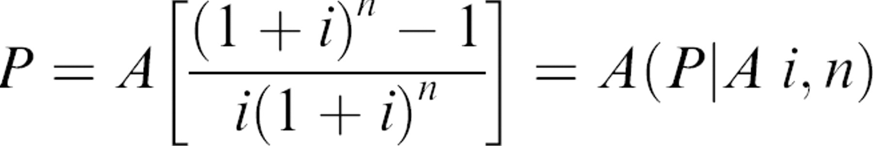
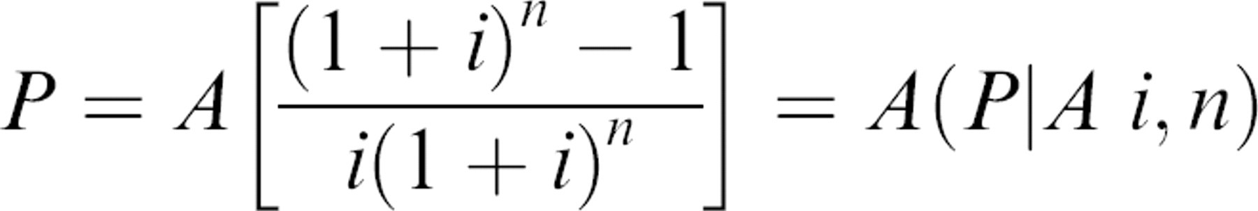
The equation for finding the present worth for a uniform series of cash flows is given as

$P\hspace{0.17em}=\hspace{0.17em}A\left[\frac{{\left(1\hspace{0.17em}+\hspace{0.17em}i\right)}^n\hspace{0.17em}-1}{i{\left(1\hspace{0.17em}+\hspace{0.17em}i\right)}^n}\right]\hspace{0.17em}=\hspace{0.17em}A\left(P|A\hspace{0.17em}i,\hspace{0.17em}n\right)$

Figure 3.

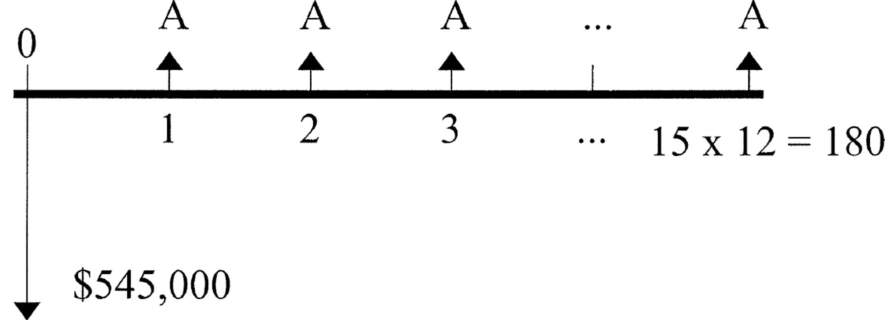
Uniform series cash flow diagram for example 4.

The notation at the right-most part of this equation is read as “the amortized amount times the factor to find the present worth given the amortized amount, at i interest per period for n interest periods. To calculate the inverse, use the capital recovery factor for a uniform series of cash flows, which is given as

$P\hspace{0.17em}=\hspace{0.17em}A\left[\frac{{\left(1\hspace{0.17em}+\hspace{0.17em}i\right)}^n\hspace{0.17em}-1}{i{\left(1\hspace{0.17em}+\hspace{0.17em}i\right)}^n}\right]\hspace{0.17em}=\hspace{0.17em}A\left(P|A\hspace{0.17em}i,\hspace{0.17em}n\right)$

In our example, an annual interest rate is quoted, but actual interest is compounded monthly. This means the annual interest rate must be converted to a monthly interest rate. Note that the interest given (i) is not the annual percentage rate (APR) from typical home or automobile loan experiences. The equation to convert annual interest to interest per n annual periods is as follows. We also show the equation with substituted values from our example.

$i_{period\hspace{0.17em}}=\hspace{0.17em}i/n_{periods\hspace{0.17em}\hspace{0.17em}}\Rightarrow \hspace{0.17em}0.07/12\hspace{0.17em}=\hspace{0.17em}0.005833\hspace{0.17em}\text{per}\hspace{0.17em}\text{period}$

Clearly, the number of interest periods per year is 12 (for monthly). Substituting i_period for i in the equations yields the following solution for example 4:

$A\hspace{0.17em}=\hspace{0.17em}\$545,000\left[\frac{0.0058{\left(1+0.0058\right)}^{180}}{{\left(1+0.0058\right)}^{180}\hspace{0.17em}-1}\right]$

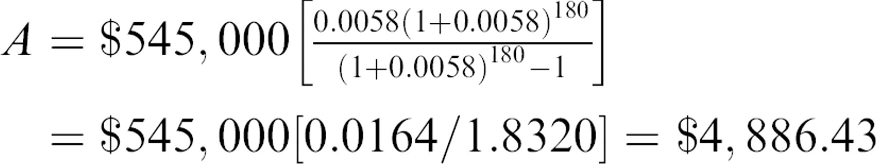
A $545,000 building would cost $4,886.43 per month with a 15-year loan at 7% annual interest (compounded monthly).

Figure 4.

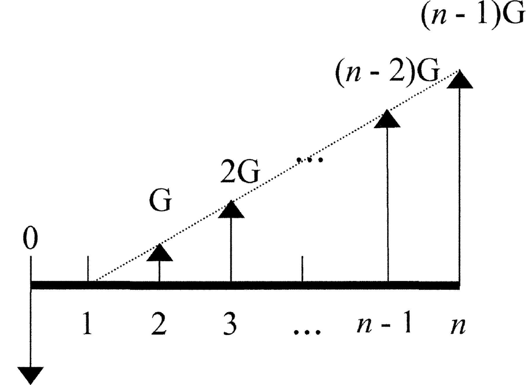
Cash flow diagram for the gradient series equations.

Other Cash Flow Series

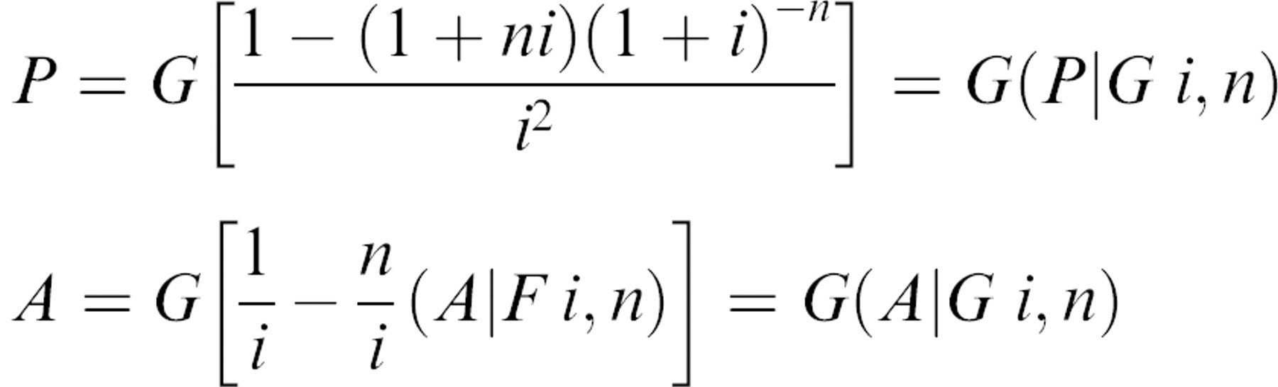
In addition to the uniform series, two other cash flow series are commonly used in economic analysis, the gradient series and the geometric series. The assumption of the gradient series is that the cash flow is increasing linearly (growth). See Figure 4 for the gradient series cash flow diagram. The geometric series assumes that cash flow is increasing geometrically. Equations for the gradient series only are presented in this tutorial since they represent more realistic behavior.

Equations for finding the present value and the amortized value for a gradient series are given as follows:

$\begin{array}{c}P\hspace{0.17em}=\hspace{0.17em}G\left[\frac{1-\left(1+ni\right){\left(1+\hspace{0.17em}i\right)}^{-n}}{i^2\hspace{0.17em}}\right]\hspace{0.17em}=\hspace{0.17em}G\left(P|G\hspace{0.17em}i,\hspace{0.17em}n\right)\\ {\rm A}=G\left[\frac{1}{i}-\frac{n}{i}\left(A|F\hspace{0.17em}i,\hspace{0.17em}n\right)\right]\hspace{0.17em}=\hspace{0.17em}G\left(A|G\hspace{0.17em}i,\hspace{0.17em}n\right)\end{array}$

Converting to an effective annual interest rate

One issue that may arise in your analyses is the need to convert from multiple compounding periods per year (m) to an effective annual interest rate (i_eff ) in order to accurately compare alternatives. This would be like determining the non-fee portion of the APR on a home or automobile loan. The equation for effective annual interest rate is as follows:

$i_{\text{eff}}\hspace{0.17em}=\hspace{0.17em}{\left(1\hspace{0.17em}+{\hspace{0.17em}}^r/m\right)}^m\hspace{0.17em}-1$

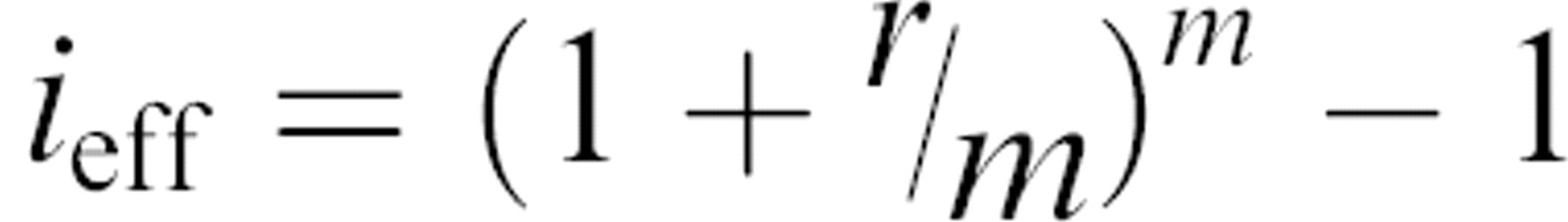
where r = the nominal annual interest rate; m = the number of compounding periods per year; and i = (r/m) = the interest rate per compounding period.

Example 5

Find the effective annual interest for a home loan of 5% compounded monthly where the quoted annual rate (r) is 5.00% (0.05) and the number of compounding periods per year (m) is 12. From the previous equation, we can calculate the effective annual interest rate as follows:

$\begin{array}{l}i=r/m=0.05/12=0.00417\hspace{0.17em}\text{interest per period}\hfill \\ i_{\text{eff}}={\left(1+r/m\right)}^m-1={\left(1+0.05/12\right)}^{12}-1\hfill \\ ={\left(1.00417\right)}^{12}-1\hfill \\ i_{\text{ef}f}=(1.0512)-1=0.0512\hspace{0.17em}\text{or}\hspace{0.17em}5.12\%\hfill \end{array}$

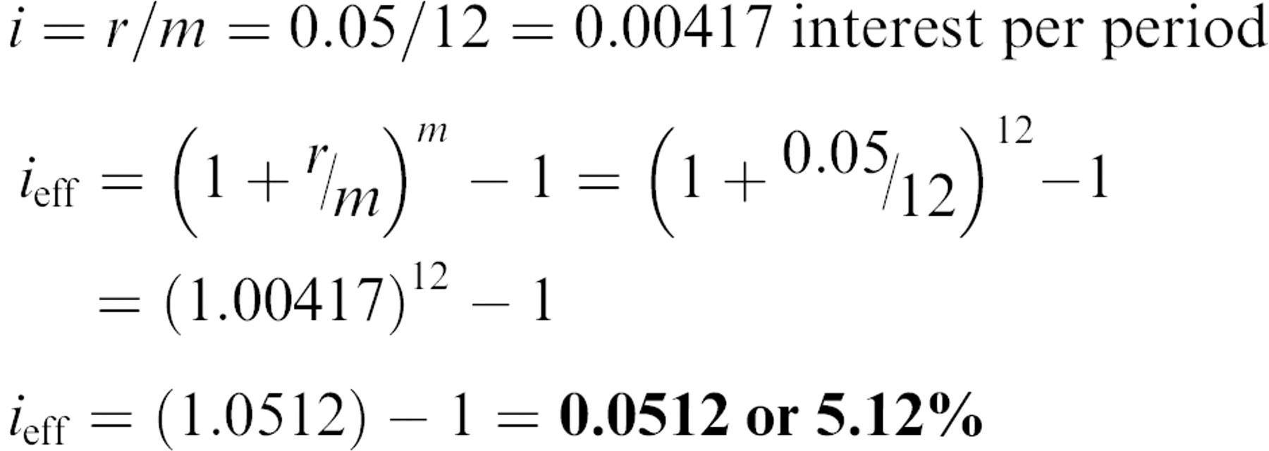
As shown by the final effective annual interest rate, a 5% nominal annual interest rate compounded monthly is equivalent to an annual compounding rate of 5.12%. The APR quoted on a loan would be 5.12% plus the backed-in measurement of the closing costs and required fees.

Inflation and Compounded Interest Rates

Inflation is a measure of the decrease in the buying power of money due to increasing costs of operations and life. This can be handled in the world of economic analysis by the following equation:

$i\hspace{0.17em}=\hspace{0.17em}d\hspace{0.17em}+\hspace{0.17em}j\hspace{0.17em}+\hspace{0.17em}d\hspace{0.17em}j$

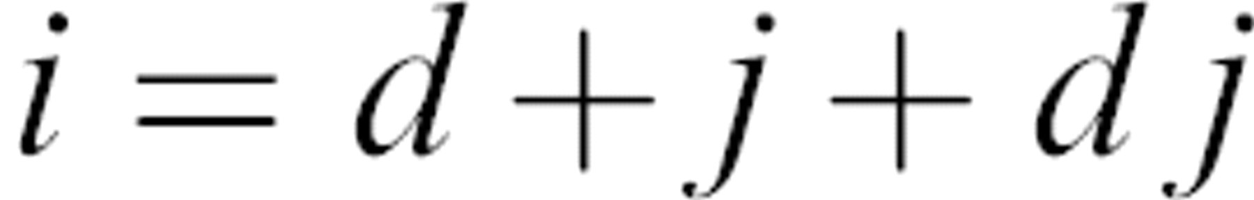
where i is the compounded interest rate, d is the base desired interest rate of return or charged, and j is the inflation rate. Following is an example showing how inflation affects interest calculations.

Example 6

To invest for a 5% return after inflation, where inflation is 1.5%, how much return is needed? Substituting into the previous equation, obtain the following.

$\begin{array}{l}i=0.05+0.015+\left(0.05*0.015\right)=0.065+\left(0.00075\right)\hfill \\ =0.06575\hspace{0.17em}\text{or}\hspace{0.17em}6.575\%\hfill \end{array}$

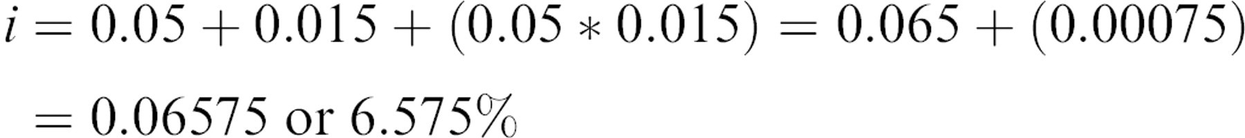
A return of 6.575% would be required to yield a 5% post inflation return on this investment.

Profitable companies use a number of metrics to help choose the most profitable projects. One way is by designating a Minimum Attractive Rate of Return (MARR). They define this percentage to take into account the company's cost of capital (the cost of raising funds via the sale of stock or loans), opportunity costs, and inflation while yielding a desired profit. Many profitable manufacturing-based companies use MARRs in the 15% to 20% range. If a company is profitable, then it will want to use the figure determined by its accounting and planning departments. Otherwise, inflation is the predominant factor. The average inflation from the Consumer Price Index (CPI) for the years 2000 through 2003 is 2.5%. Note that this is a historically low rate. Because I have observed that laboratory equipment prices seem to increase a little ahead of the CPI, I use 3% as the inflation rate if my accounting department does not have a number for me to use. Estimates for projects with a 5- or 10-year time span probably should use a higher inflation rate that is more in line with typical rates, such as 5%.

Filling Out the Costs of Laboratory Automation and Research

The first step to take when performing an economic analysis of laboratory automation is to identify costs.

Direct Costs of People

The people who work on a project, in a lab or on a product, must be considered direct costs and must be included in any analysis. Indirect personnel, such as administrative, purchasing, safety, facilities support, top management, are not considered, as they are not changed by the choice of laboratory automation.

Table 2 presents a summation of biotech salaries for a number of hotbed locations from Salary.com ⁴ for U.S. jobs and WetFeet.com ^5,6 for European jobs, based on 2002 data. Even though the number may not be completely accurate, a 2080-hour work year can be used to determine hourly costs. Please note that all of these figures are based on incomes prior to this current year. The U.S. is experiencing downward pressure on salaries due to a large number of lay-offs in the pharma and biotech sectors; therefore, scientist salaries appear inflated. An individual company's accounting or planning departments should be able to provide more accurate numbers to use in cost calculations.

Table 2.

Yearly and hourly salaries for a number of titles and locations

	Median Salaries – Yearly and (hourly – rounded) in $U.S., based on 2002 data.
		Note: these figures do not include benefits.
Job title and years experience	San Diego, CA	San Francisco, CA	Boston, MA	England (Average)	Switzerland (Average)
Engineer II 2–5 years	$65,549 ($31)	$72,993 ($35)	$68,051 ($33)
Engineer III 5–8 years	$78,960 ($38)	$87,926 ($42)	$81,974 ($39)
Research Associate I 0–2 years	$38,457 ($18)	$42,824 ($20)	$39,925 ($19)
Research Associate II 2–5 years	$47,394 ($23)	$52,046 ($25)	$48,523 ($23)
Research Associate III 5+ years	$57,886 ($28)	$64,458 ($31)	$60,095 ($29)
Scientist II 3–5 years	$83,138 ($40)	$92,578 ($44)	$86,311 ($41)
Scientist III 6+ years	$96,339 ($46)	$107,278 ($51)	$100,016 ($48)
Research Technician all levels				$27,666 ($13)	$63,473 ($30)
Biologist all levels				$42,830 ($20)	$101,622 ($49)
Chemist all levels				$38,656 ($18)	$96,440 ($46)
Mechanical engineer all levels				$44,496 ($21)	$110,925 ($53)

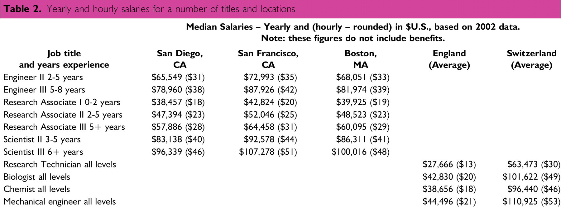
Benefits and employment taxes add to these figures. From conversations with a variety of human resources departments, in the case of California, 1.4 is a good multiplier to determine the realistic direct employment costs to a company. In other parts of the U.S., 1.30 is a more accurate multiplier. In Europe, the employment cost can be greater than a factor of 1.50. Ideally, the human resources, personnel, or accounting departments should provide an accurate multiplier.

Direct Costs of Equipment (U.S. Bias)

Following is a list of equipment price ranges based on U.S. pricing. This can be very different in Europe or Asia, especially for purchases made through a distributor. These are considered direct costs.

• Pipetting robot: $25,000–$200,000

• 96 Channel pipetting robot: $20,000–$200,000

• Robot arm: $14,000–$55,000

• Pre-integrated off-the-shelf system: $150,000–$750,000

• Custom integrated major system: $1,000,000–$10,000,000

• Refrigerated robot accessible plate storage: $30,000–$180,000

• Carousel: $10,000–$30,000

• Plate stacker: $10,000–$30,000

• Service contracts average 10% of the purchase price per year

Indirect Costs of Equipment

Many users of laboratory automation do not consider related safety issues. While this may be acceptable for workstations, safety considerations and their associated costs must be taken into account for large integrated systems. If the system does not come with protection for personnel, the company must install it. For the U.S., the best reference is the standard titled, ANSI/RIA R15.06–1999, American National Standard for Industrial Robots and Robot Systems - Safety Requirements (revision of ANSI/RIA R15.06–1992). This publication is available from the Robotic Industries Association (Ann Arbor, MI, USA). ⁷ This document includes case studies and new standards. It is the definitive reference for the U.S. and is often used by the Occupational Safety & Health Administration (OSHA). It explains how to prevent injuries and possible claims by using interlocks, barriers, and tagout systems. Europe has other standards ¹¹ .

Scalable Indirect Costs of People

Another, even more insidious cost is that of repetitive motion injuries (RMIs). Also known as repetitive strain injuries, or by OSHA as musculoskeletal disorders (MSDs) ⁸ and by other names, these injuries are a common problem in mass-production environments. Manual laboratory equipment is especially notorious for causing RMI problems. Frequently, the cost of automating a high-RMI risk activity is too expensive. Therefore, for a high-risk activity that is causing RMIs, work should focus on automating as many tasks as possible (prioritizing those that are the least expensive to implement) to reduce the overall risk of causing RMIs. Here is why: Each RMI incident that doesn't involve lawsuits can cost a company approximately $30,000 in time spent throughout the organization dealing with it, retraining, and, occasionally, rehiring. From informal studies at a number of companies, every year it can be assumed that one out of every five employees working on a risky (i.e., uncomfortable) task will have RMI problems. Pepperidge Farm confirmed this number ⁹ in a 2001 presentation at a robotics conference, but it is one of those statistics that few companies will acknowledge publicly. This cost must be included in the cost estimates for people, especially for non-automated alternatives.

Costs of Consumables

Consumables can be the most expensive part of any chemical or biochemical process. These costs scale with the number of experiments or processes performed and therefore are variable costs. As anyone doing research in pharma, biotechnology, or academia is aware, reagents can be very costly. Currently, a popular example of this is Taq Polymerase, the enzyme used to copy DNA during a PCR reaction. The disposable single-use labware items that are often utilized are costly and can range from microtiter plates, to synthesis columns, to weighing bottles.

While these costs are obvious, the costs involved in disposing of these consumables are often overlooked. Chemical and radioactive hazard disposal can be very expensive. Some chemicals can be more expensive to get rid of as waste than they were to purchase. Even with a decay storage area for low-grade radioactive waste, space and monitoring have costs associated with them. Even non-hazardous trash disposal has a cost. Usually a company's accounting department or waste disposal group can provide an average multiplier to account for costs associated with disposing of chemical, radioactive, and even non-hazardous lab-waste.

In addition, there can be other consumables such as gasses and purified water. When managed properly, these consumables, along with compressed air or vacuums, can be supplied by the equipment that is purchased once and then maintained. One of the oft-stated goals of automating a laboratory process is to reduce the cost of consumables, usually by reducing the size of reactions. However, one of the main advantages of laboratory automation is actually that of reducing experimental error.

Costs of Experimental Errors

Ideally, experiments and processes are designed to clearly discern between errors and data. If so, then current error rates can be determined. In many companies and research environments, this number is more politically difficult to admit than it is to determine. One employer determined that its experimental error rate for a process was 50%, leading to 100% re-runs of the experiments. Automating the processes cut this to 10%. Improving the quality and quality control of the reagents cut this to 3%. In reducing this error, costs also were reduced and throughput was increased, finally rerunning 3% of experiments. Product manufacturing can approach “six-sigma” quality, meaning almost zero defective products. This is essentially impossible for “discovery” projects. By definition, not everything is known about the process, so more errors will occur. Experience suggests the following error rates for genomic and chemical discovery processes:

• Manual: 10%–30%. Manual operations equal manual mistakes, especially due to boredom or fatigue.

• Islands of Automation (workstation based): 1–10%. Mistakes still happen, but much less often. They do affect more samples when they happen.

• Full Automation (integrated system based): l%–5%. Mistakes happen very rarely but affect a large number of samples very quickly.

Mistakes create additional expenses. To compensate, cost estimates for running a process or experiment need to be inflated by one plus the error rate.

Example 7

An experimental process costs a projected $1600 per day to run in consumables alone. With an experimental error rate of 10%, how much would it cost in consumables to get all of the data? A 10% error rate means 10% more experiments must be run, using 110% of expected reagents. Therefore, the actual cost of the experiments is calculated as follows:

$\$1600\hspace{0.17em}\times \hspace{0.17em}\left(1.10\right)\hspace{0.17em}=\hspace{0.17em}\$1760\hspace{0.17em}\text{per}\hspace{0.17em}\text{day}$

For this, we can see that error rate is an inflationary cost.

Costs of Equipment Reliability

Reliability is the percentage of time that a piece of equipment or component is capable of performing its function. There is an entire branch of engineering dedicated to reliability, especially aimed at the aerospace fields. Availability is reliability minus the time needed for maintenance and repairs. Unfortunately, laboratory automation equipment manufacturers do not supply these numbers, so the best bet is to ask for references. To determine a percentage, current users can estimate, on average, how many hours a day their equipment actually runs, less setup and regular maintenance time. Remember that most workstations are usable only while people are present.

Example 8

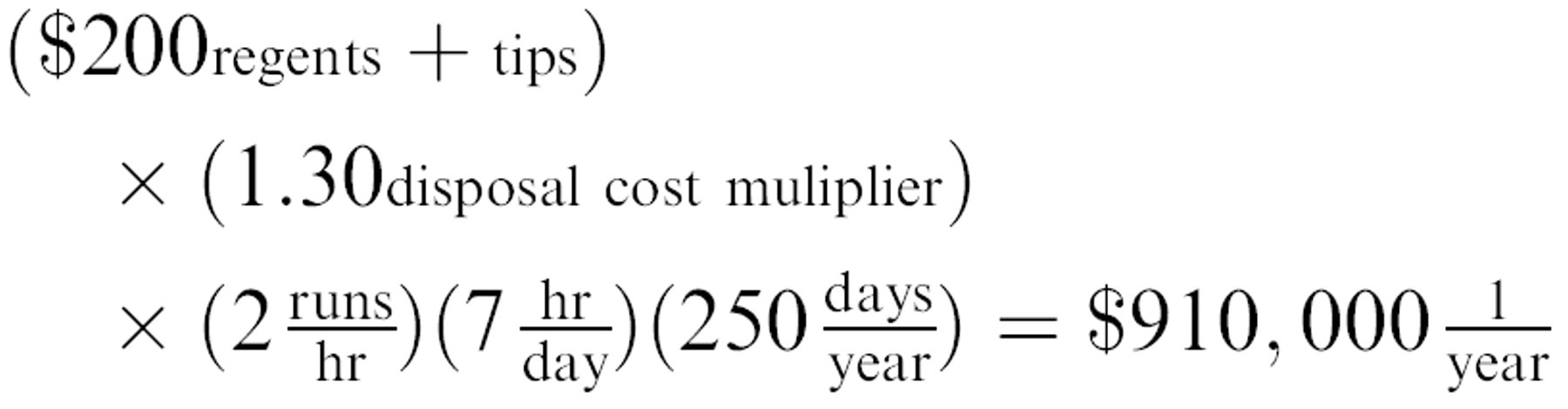
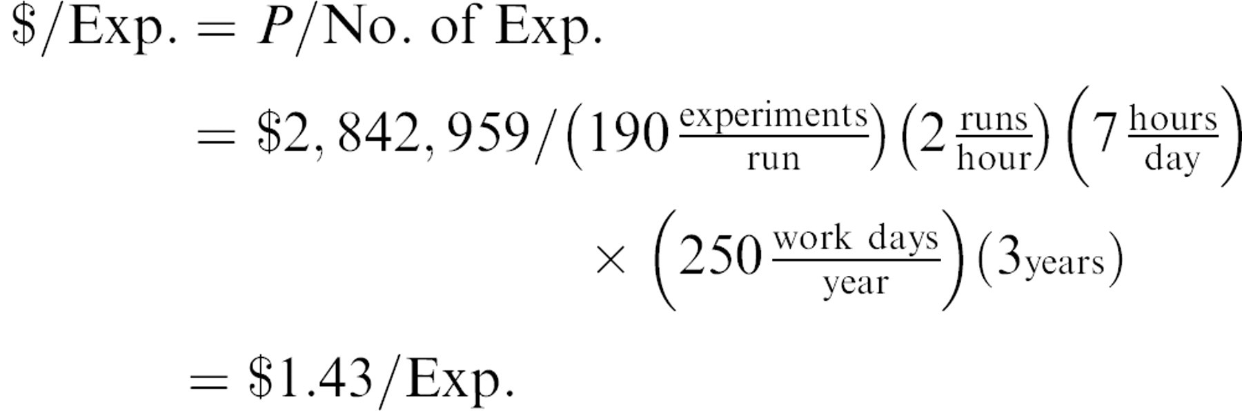
An ELISA assay can be automated on a liquid handling robot for $63,000. The robot will be used in a workstation mode. One research associate will be able to operate and support two systems. The cost per run in reagents, labware, and disposable tips is $200, plus an additional 30% for monitoring and disposal. Assume two runs per hour, 7 hours a day, 250 days per year.

What is the present worth cost per experiment for a three year planned useful life of the experimental method used, assuming 190 experiments per run? Factor in an interest rate of 3% compounded annually. To solve this problem, first convert operating costs to an annual basis. The costs of reagents per year is calculated as:

$\begin{array}{c}\left(\${200}_{\text{regents}\hspace{0.17em}}+\hspace{0.17em}\text{tips}\right)\\ \times \hspace{0.17em}\left({1.30}_{disposal\hspace{0.17em}cost\hspace{0.17em}muliplier}\right)\\ \times \hspace{0.17em}\left(2\frac{\text{runs}}{\text{hr}}\right)\hspace{0.17em}\left(7\frac{\text{hr}}{\text{day}}\right)\hspace{0.17em}\left(250\frac{\text{days}}{\text{year}}\right)\hspace{0.17em}=\hspace{0.17em}\$910,000\frac{1}{\text{year}}\end{array}$

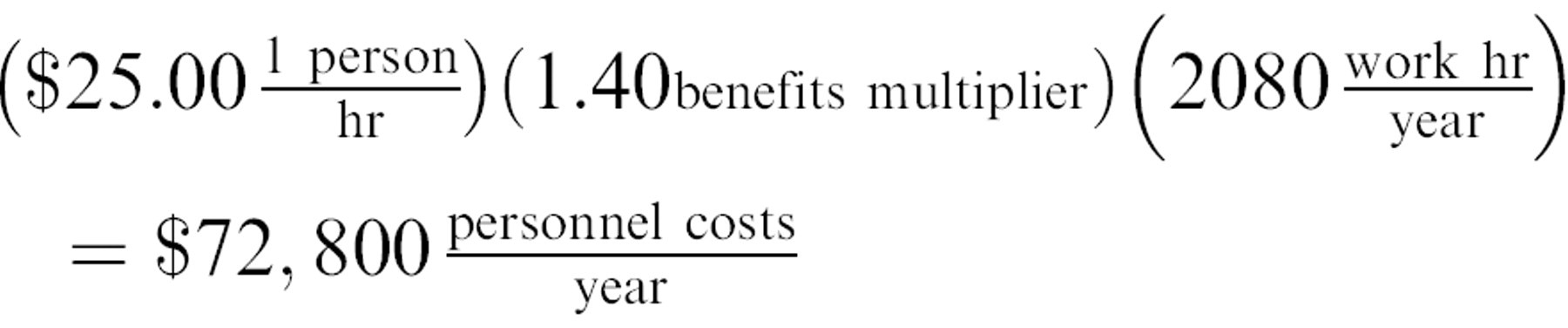
From the information given, we use $25/hr + 40% for the wages paid plus benefits. Then, the costs of personnel per year is calculated as:

$\begin{array}{c}\left(\$25.00\frac{1\hspace{0.17em}\text{person}}{\text{hr}}\right)\left(1.40\hspace{0.17em}\text{benefits}\hspace{0.17em}\text{multiplier}\right)\left(2080\frac{\text{work}\hspace{0.17em}\text{hr}}{\text{year}}\right)\\ =\$72,800\hspace{0.17em}\frac{\text{personnel}\hspace{0.17em}\text{costs}}{\text{year}}\end{array}$

The cash flow diagram for this problem is depicted in Figure 5.

Figure 5.

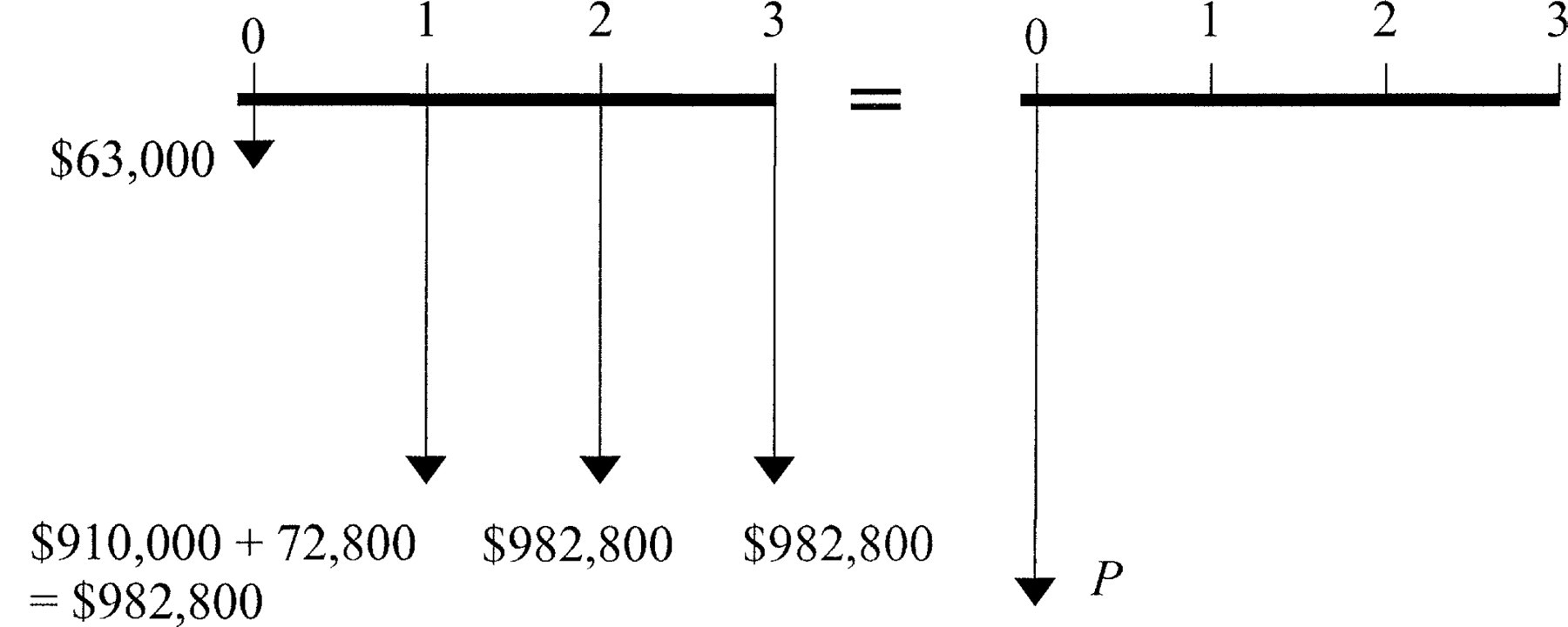
Cash flow diagram for example 8.

Solving for equivalent present worth (P) and then dividing by the number of experiments per three years, obtain:

$\begin{array}{lll}P\hfill & =\hfill & \$63,{000}_{\text{first}\hspace{0.17em}\text{cost}}+\$982,{800}_{\text{annual}\hspace{0.17em}\text{cost}}\left(P|A\hspace{0.17em}i,\hspace{0.17em}n\right)\hfill \\ \hfill & =\hfill & \$63,{000}_{\text{first}\hspace{0.17em}\text{cost}}+\$982,{800}_{\text{annual}\hspace{0.17em}\text{cost}}\left[\frac{{\left(1+i\right)}^n-1}{i{\left(1+i\right)}^n}\right]\hfill \\ \hfill & =\hfill & \$63,{000}_{\text{first}\hspace{0.17em}\text{cost}}+\$982,{800}_{\text{annual}\hspace{0.17em}\text{cost}}\left[\frac{{\left(1.03\right)}^3-1}{0.03{\left(1.03\right)}^3}\right]\hfill \\ \hfill & =\hfill & \$(63,{000}_{\text{first}\hspace{0.17em}\text{cost}}\hfill \\ \hfill & \hfill & \hspace{1em}+982,{800}_{\text{annual}\hspace{0.17em}\text{cost}}\left(\frac{0.092727}{0.032782}\right))=\$2,842,959\hfill \end{array}$

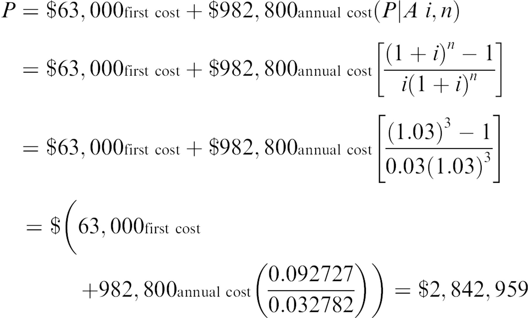
This yields a present worth (P) of $2,842,959. Note that rounding differences become evident with this number.

Next, to determine the cost per experiment in today's money, perform the following calculation:

$\begin{array}{l}\$/\text{Exp}.=P/\text{No}.\hspace{0.17em}\text{of}\hspace{0.17em}\text{Exp}.\hfill \\ \hspace{0.17em}\hspace{0.17em}\hspace{0.17em}\hspace{0.17em}\hspace{0.17em}\hspace{0.17em}\hspace{0.17em}\hspace{0.17em}\hspace{0.17em}\hspace{0.17em}\hspace{0.17em}=\$2,842,959/\left(190\frac{\text{experiments}}{\text{run}}\right)\left(2\frac{\text{runs}}{\text{hour}}\right)\left(7\frac{\text{hours}}{\text{day}}\right)\hfill \\ \hspace{0.17em}\hspace{0.17em}\hspace{0.17em}\hspace{0.17em}\hspace{0.17em}\hspace{0.17em}\hspace{0.17em}\hspace{0.17em}\hspace{0.17em}\hspace{0.17em}\hspace{0.17em}\hspace{0.17em}\hspace{0.17em}\hspace{0.17em}\hspace{0.17em}\hspace{0.17em}\hspace{0.17em}\hspace{0.17em}\hspace{0.17em}\hspace{0.17em}\hspace{0.17em}\hspace{0.17em}\hspace{0.17em}\hspace{0.17em}\hspace{0.17em}\hspace{0.17em}\hspace{0.17em}\hspace{0.17em}\hspace{0.17em}\hspace{0.17em}\hspace{0.17em}\hspace{0.17em}\hspace{0.17em}\times \left(250\frac{\text{work}\hspace{0.17em}\text{days}}{\text{year}}\right)\left(3\text{years}\right)\hfill \\ \hspace{0.17em}\hspace{0.17em}\hspace{0.17em}\hspace{0.17em}\hspace{0.17em}\hspace{0.17em}\hspace{0.17em}\hspace{0.17em}\hspace{0.17em}\hspace{0.17em}\hspace{0.17em}=\$1.43/\text{Exp}.\hfill \end{array}$

Comparing Alternatives: Manual, Islands of Automation, and Full Automation

Alternatives to laboratory operations include manual processes, islands of automation using workstation-based liquid handling robots, and full automation based on an integrated system. There are a number of ground rules to consider when comparing these alternatives:

• Compare the present worth of the total cost of the system. This can be divided by the number of successful experiments for comparing to outside sources.

• Factor inflation for laboratory equipment averaged over the previous three years at 3% (the CPI has gone up 2.5% averaged over the same time). ¹⁰ Note that if a company is profitable, it should use the Minimum Attractive Rate of Return (MARR), as determined by its accounting and/or planning department.

• Take into account the opportunity cost of dedicating people to a task. The simplest way to accomplish this is to double their salaries and benefits. This captures the need to hire more people with the same capabilities to perform other tasks.

• Assume one RMI incident per five people at a $30,000 cost per incident for manual labor.

• Assume that service contracts for equipment remain at the same price over two to three years.

• For the sake of simplicity, assume that wages increase at the same rate as other costs, i.e., 3%.

The islands of automation methods are not appreciably faster than manual methods. All savings must come from decreased error rates or off-hour use. Larger or full automation systems can be expected to run without human help during off hours and can process samples faster than people.

Example 9

Compare the three lab process alternatives (manual, islands of automation, and full automation) under the following conditions:

Manual Method

Labor

• Single shift: Note that it may be very difficult to hire scientists willing to work second or third shift. Moreover, it may require a shift differential of perhaps 10% for the second shift and more for the night shift.

• 10 people total: 6 Research Associate Is under the supervision of 4 Research Associate IIs.

• Assume two RMI incidents per year.

Equipment

• Manual tools (pipettes, pipetters and others): 10 sets for a total of $6,000.

• Analysis equipment: $15,000.

• Off-line cold storage is the same for all three alternatives, so it can be neglected.

Error rate

• As mentioned, manual methods with complicated processes can create error rates that range from 10 to 30%. For this example, use 15%.

Experimental rate

• 96 well-plate-based, 10 plates per hour, 7 hours per day (assume one lost hour per day).

• Availability = 100%.

Islands of Automation

Labor

• Assume a single shift.

• 6 people total: 4 Research Associate Is under the supervision of 2 Research Associate IIs + $3000 in training for 2 people.

• No RMI.

Equipment

• Manual tools: 4 sets, for a total of $3,500 for touch-up or in case of emergency.

• Analysis equipment: $15,000.

• Three high-end liquid transfer robots: $85,000 each.

Error rate

• As mentioned, islands of automation can create error rates from 1% to 10% through the incorrect set-up of robots, disposable problems, and reagent failures. For this example, use 3%.

Experimental rate

• 96 well-plate-based, 10 plates per hour (for all three systems combined), 7 hours per day.

• Availability = 95% (maintenance plus breakdowns).

Full or Integrated Automation

Labor

• Assume a single shift.

• 2 people total: 2 Research Associates (one is a III so add $3/hr) + $5,000 for training.

• No RMI.

Equipment

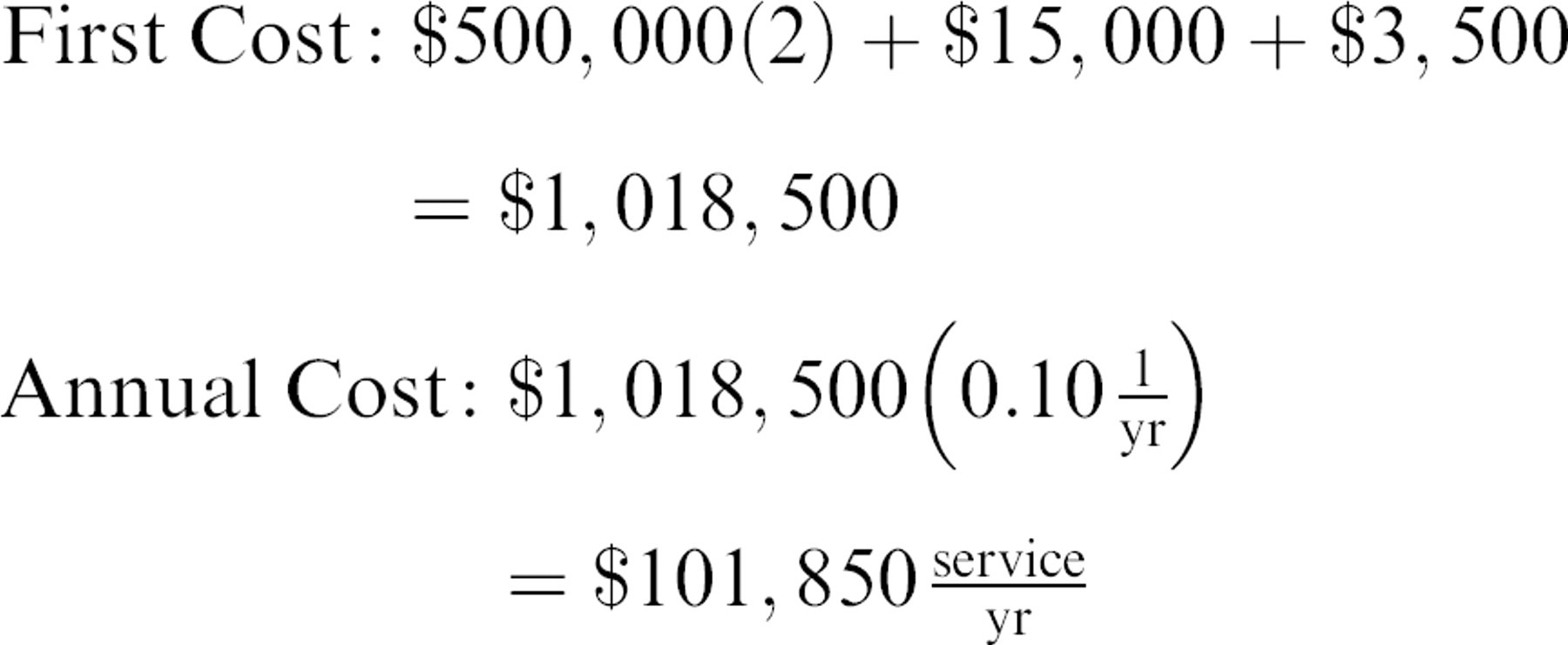
• Manual tools: 4 total, for a total of $3,500 for touch-up or in case of emergency.

• Two semi-custom integrated automation systems, including on-line refrigerated storage and analysis, $500,000 each.

Error rate

• As mentioned, full automation can be expected to generate an error rate of between 1 and 5%. Although mistakes happen much less often, many more samples are affected with each incident. For this example, use 3%, assuming disposables problems.

Experimental rate

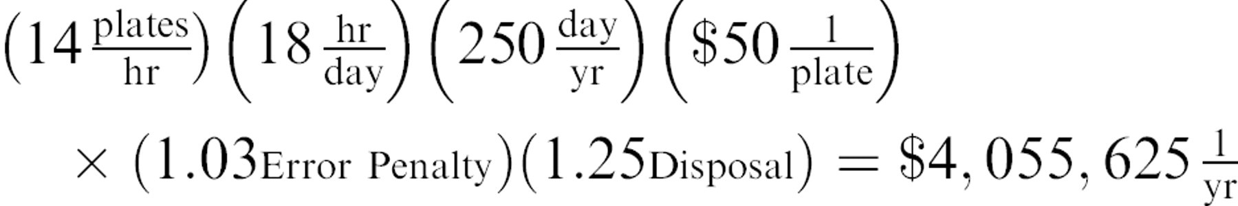
• 96 well-plate-based, 14 plates per hour (7 a piece), 18 hours per day, including the overnight run.

• Availability is 85%. Remaining time accounts for maintenance plus breakdowns.

General Assumptions

Labor

Use the following numbers for labor rates. These do not correspond to numbers given previously.

• Research Associate I, $18/hr.

• Research Associates (II), $25/hr and (III), $28/hr.

• Add 40% for benefits and taxes.

Equipment

• All equipment has a 10% per year support cost.

Error Rate

• Add the error rate to all continuing costs as the penalty incurred when required to rerun experiments.

Length of Project

• For manual and islands of automation, assume 3 years for this experimental method.

• For full automation, assume 2 years due to higher throughput meeting scientific goals.

Reagents and Disposables

• Assume a cost of $50 per plate, plus 25% for monitoring and disposal.

Interest rate

• Assume 3% interest, compounded annually.

To solve the comparison problem for each alternative, we calculate labor costs, the costs of reagents and disposables, and equipment costs, all on an annual basis. Next, we draw the cash flow diagram and then solve for present worth. When calculations for all three alternatives are complete, the option with the smallest nominal present worth is the economically preferred choice, because it implies the smallest expense. Let us take each method in turn.

Manual Method For the manual method alternative, the annual costs for labor, reagents and disposables, and equipment can be calculated as follows:

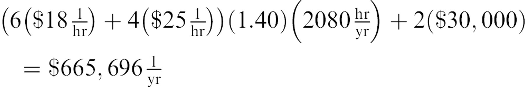
Labor costs:

$\begin{array}{c}(6\left(\$18\frac{1}{\text{hr}}\right)\hspace{0.17em}4\left(\$25\frac{1}{\text{hr}}\right))\hspace{0.17em}\left(1.40\right)\hspace{0.17em}\left(2080\frac{\text{hr}}{\text{yr}}\right)\hspace{0.17em}+\hspace{0.17em}2\left(\$30,000\right)\\ =\$665,696\frac{1}{\text{hr}}\end{array}$

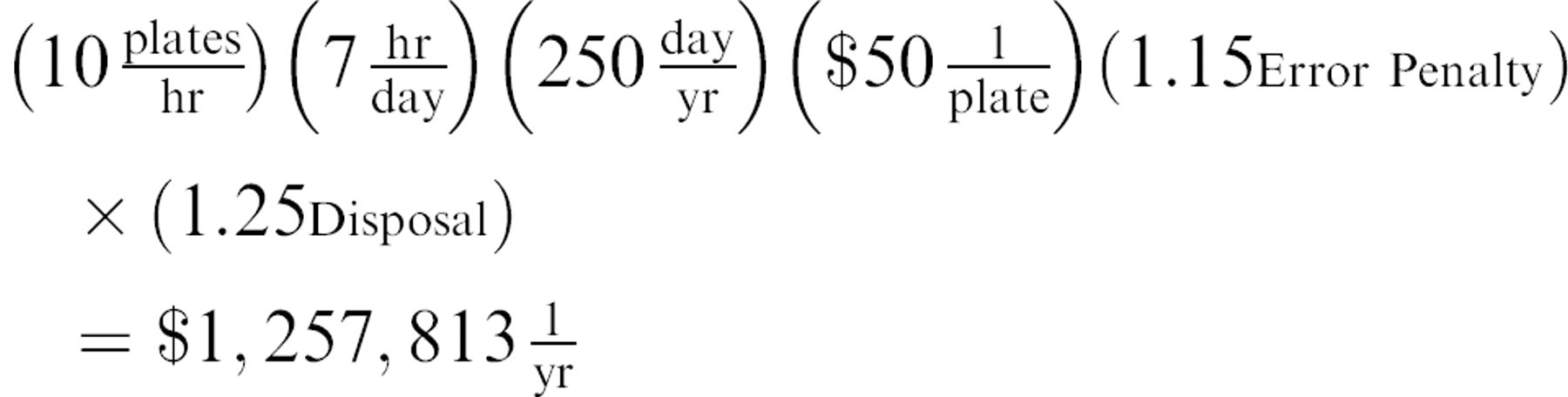
Reagent and disposables costs:

$\begin{array}{c}\left(10\frac{\text{plates}}{\text{hr}}\right)\left(7\frac{\text{hr}}{\text{day}}\right)\left(250\frac{\text{day}}{\text{yr}}\right)\left(\$50\frac{\text{1}}{\text{plate}}\right)\hspace{0.17em}\hspace{0.17em}\left({1.15}_{\text{Error}\hspace{0.17em}\text{Penalty}}\right)\hspace{0.17em}\hspace{0.17em}\\ \times \hspace{0.17em}\left({1.25}_{\text{Disposal}}\right)\\ \$1,257,813\frac{1}{\text{yr}}\end{array}$

Equipment costs:

$\begin{array}{l}\text{First}\hspace{0.17em}\text{Cost}:\hspace{0.17em}\$6,000+\$15,000=\$21,000\hfill \\ \text{Annual}\hspace{0.17em}\text{Cost}:\hspace{0.17em}\$21,000\left(0.10\frac{\text{service}}{\text{yr}}\right)=\$2,100\frac{1}{\text{yr}}\hfill \end{array}$

The cash flow diagram for the manual method is depicted in Figure 6. Solving for the present worth gives the following result:

$\begin{array}{l}\begin{array}{l}\begin{array}{l}{P}_{Manual}=\$21,{000}_{\text{first}\hspace{0.17em}\text{cost}}+\$1,925,{609}_{\text{annual}\hspace{0.17em}\text{cost}}\left(P|Ai,n\right)\hfill \\ =\$21,{000}_{\text{first}\hspace{0.17em}\text{cost}}+\$1,925,{609}_{\text{annual}\hspace{0.17em}\text{cost}}\left[\frac{{\left(1+i\right)}^n-1}{i{\left(1+i\right)}^n}\right]\hfill \end{array}\hfill \\ =\$21,{000}_{\text{first}\hspace{0.17em}\text{cost}}+\$1,925,{609}_{\text{annual}\hspace{0.17em}\text{cost}}\left[\frac{{\left(1.03\right)}^2-1}{0.03{\left(1.03\right)}^3}\right]\hfill \\ \$\left(21,{000}_{\text{first}\hspace{0.17em}\text{cost}}+\$1,925,{609}_{\text{annual}\hspace{0.17em}\text{cost}}\left(\frac{0.092727}{0.032782}\right)\right)\hfill \end{array}\hfill \\ =\$5,467,768\hfill \\ \hfill \end{array}$

Figure 6.

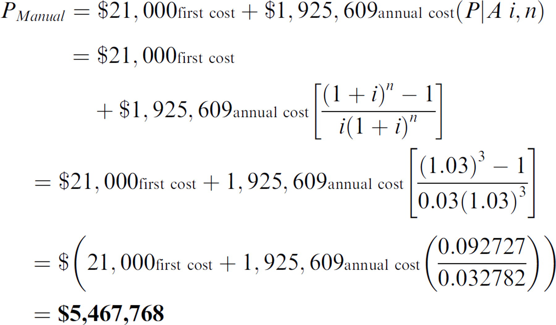
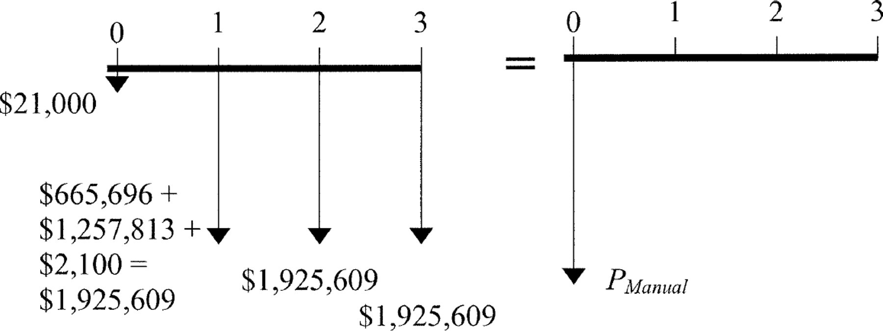
Cash flow diagram for the manual method of example 9.

Islands of Automation Method In a similar manner, first calculate costs for labor, reagents and disposables, and equipment:

Labor Costs:

$\left(4\left(\$18\frac{1}{\text{hr}}\right)+2\left(\$25\frac{1}{\text{hr}}\right)\right)\left(1.40\right)\left(2080\frac{\text{hr}}{\text{yr}}\right)=\$355,264\frac{1}{\text{yr}}$

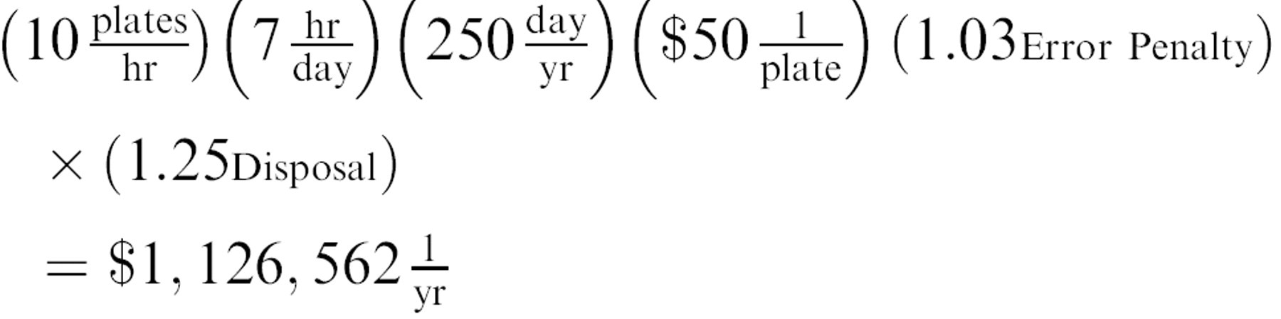
Reagent and disposables costs:

$\begin{array}{l}\left(10\frac{\text{plates}}{\text{hr}}\right)\left(7\frac{\text{hr}}{\text{day}}\right)\left(250\frac{\text{day}}{\text{hr}}\right)\left(\$50\frac{1}{\text{plate}}\right)\left({1.03}_{\text{Error}\hspace{0.17em}\text{Penalty}}\right)\times \left({1.25}_{\text{Disposal}}\right)\hfill \\ =\$1,126,562\frac{1}{\text{yr}}\hfill \end{array}$

Equipment costs:

$\begin{array}{l}\begin{array}{c}\text{First}\hspace{0.17em}\text{Cost}:\$\text{85},\hspace{0.17em}\text{000}\left(3\right)+\hspace{0.17em}\text{\$15},\text{000}+\hspace{0.17em}\$3,500\\ =\hspace{0.17em}\$273,500\end{array}\\ \text{Annual}\hspace{0.17em}\text{Cost}:\hspace{0.17em}\$273,500\left(0.10\frac{1}{\text{yr}}\right)\hspace{0.17em}=\$27,350\frac{1}{\text{yr}}\end{array}$

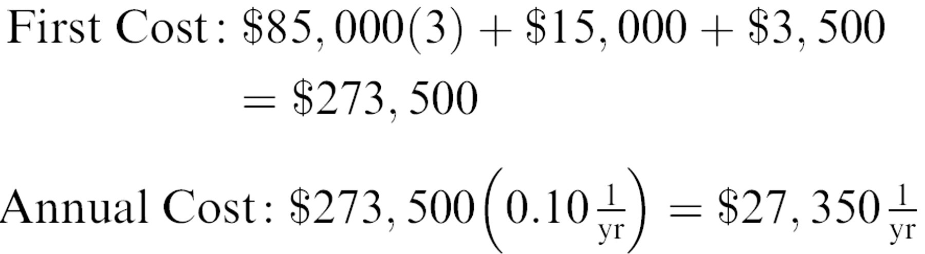
Figure 7 depicts the cash flow diagram for the islands of automation alternative.

Solving for the present worth gives the following results.

$\begin{array}{c}{P}_{islands\hspace{0.17em}}=\hspace{0.17em}\$276,{500}_{\text{firstcost}}\hspace{0.17em}\hspace{0.17em}+\hspace{0.17em}\$1,509,{176}_{\text{annual}\hspace{0.17em}\text{cost}}\hspace{0.17em}\left(P|A\hspace{0.17em}i,\hspace{0.17em}n\right)\\ =\hspace{0.17em}\$276,\hspace{0.17em}{500}_{\text{first}\hspace{0.17em}\text{cost}\hspace{0.17em}}+\hspace{0.17em}\$1,509,{176}_{\text{annual}\hspace{0.17em}\text{cost}\hspace{0.17em}}\left[\frac{{\left(1+i\right)}^n\hspace{0.17em}-\hspace{0.17em}1}{i{\left(1\hspace{0.17em}+i\right)}^n}\right]\\ \$276,{500}_{\text{first}\hspace{0.17em}\text{cost}\hspace{0.17em}}+\$1,509,{176}_{\text{annual}\hspace{0.17em}\text{cost}}\hspace{0.17em}\left[\frac{{\left(1.03\right)}^3\hspace{0.17em}-\hspace{0.17em}1}{0.03{\left(1.03\right)}^3}\right]\hspace{0.17em}\\ =\$\left(276,{500}_{\text{first}\hspace{0.17em}\text{cost}\hspace{0.17em}}+\$1,509,{176}_{\text{annual}\hspace{0.17em}\text{cost}\hspace{0.17em}}\left(\frac{0.092727}{0.032782}\right)\right)\\ =\$4,545,348\end{array}$

Figure 7.

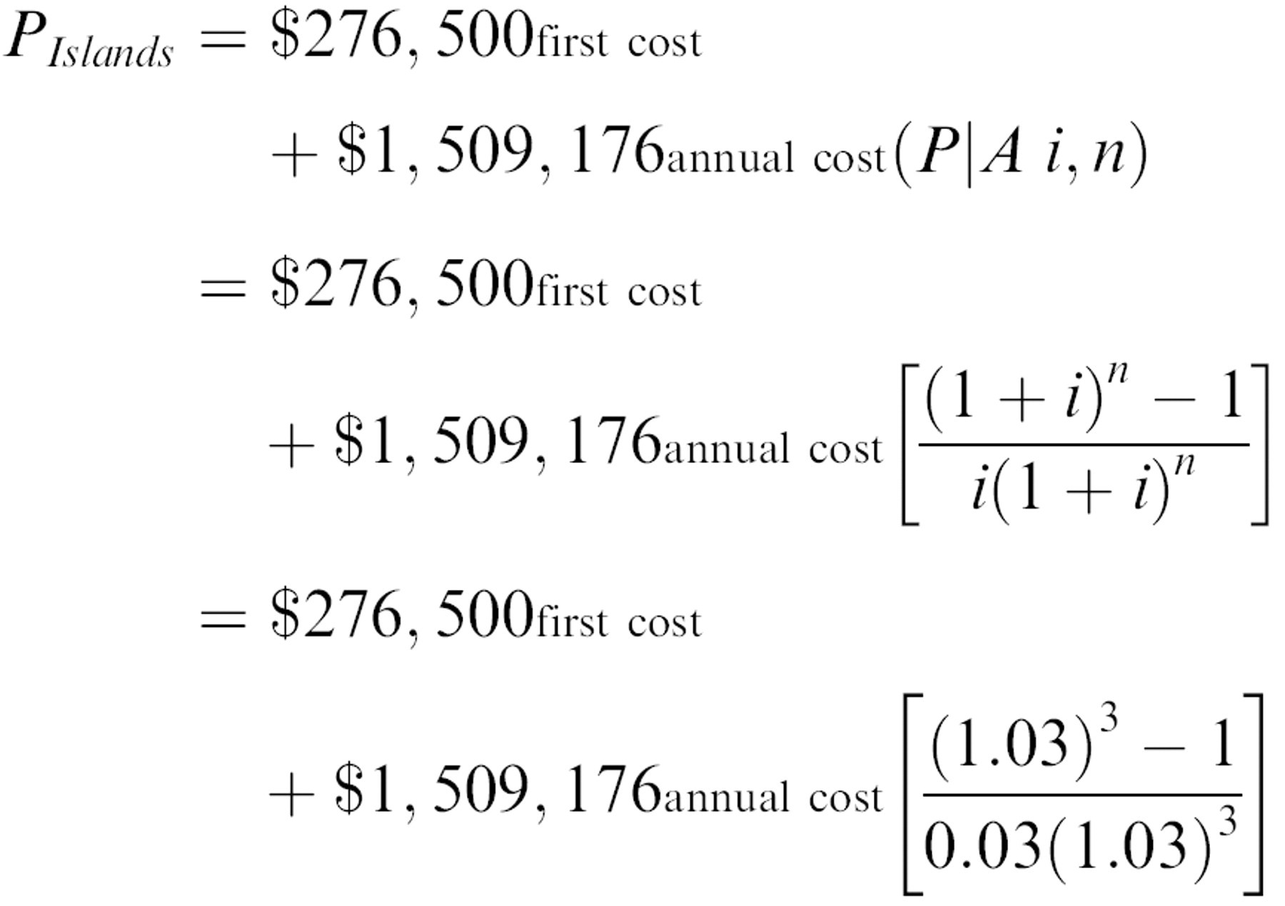
Cash flow diagram for the islands of automation method of example 9.

Full Automation Method

Labor costs:

$\left(\$25+\left(\$25+\$3\right)\right)\frac{1}{hr}\left(1.40\right)\left(2080\frac{hr}{yr}\right)=\$1,54,336\frac{1}{yr}$

Reagent and disposables costs:

$\begin{array}{l}\left(14\frac{plates}{hr}\right)\left(18\frac{hr}{day}\right)\left(250\frac{day}{yr}\right)\left(\$50\frac{1}{plate}\right)\\ \hspace{0.17em}\hspace{0.17em}\hspace{0.17em}\hspace{0.17em}\hspace{0.17em}\times \left({1.03}_{\text{Error}\hspace{0.17em}\text{penalty}}\right)\left({1.25}_{\text{Disposal}}\right)=\$4,055,625\frac{1}{yr}\end{array}$

Equipment costs:

$\hspace{0.17em}\begin{array}{c}\text{First}\hspace{0.17em}\text{Cost}:\hspace{0.17em}\$500,000\left(2\right)\hspace{0.17em}+\hspace{0.17em}\$15,000\hspace{0.17em}+\hspace{0.17em}\$3,500\\ =\hspace{0.17em}\$1,\hspace{0.17em}018,\hspace{0.17em}500\\ \text{Annual}\hspace{0.17em}\text{Cost}:\hspace{0.17em}\$1,018,500\left(0.10\frac{1}{\text{yr}}\right)\hspace{0.17em}\\ =\hspace{0.17em}\$101,850\frac{\text{service}}{\text{yr}}\end{array}$

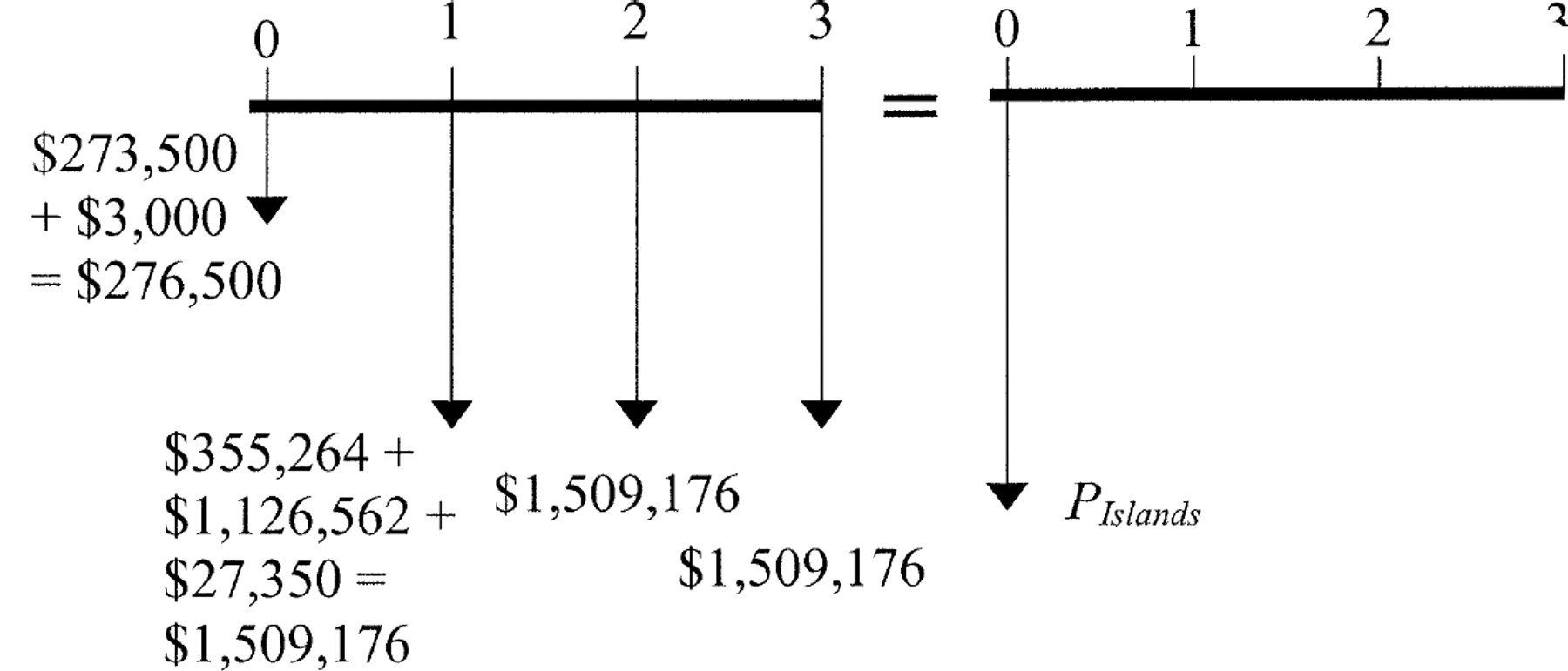
The cash flow diagram for the full automation method is depicted in Figure 8.

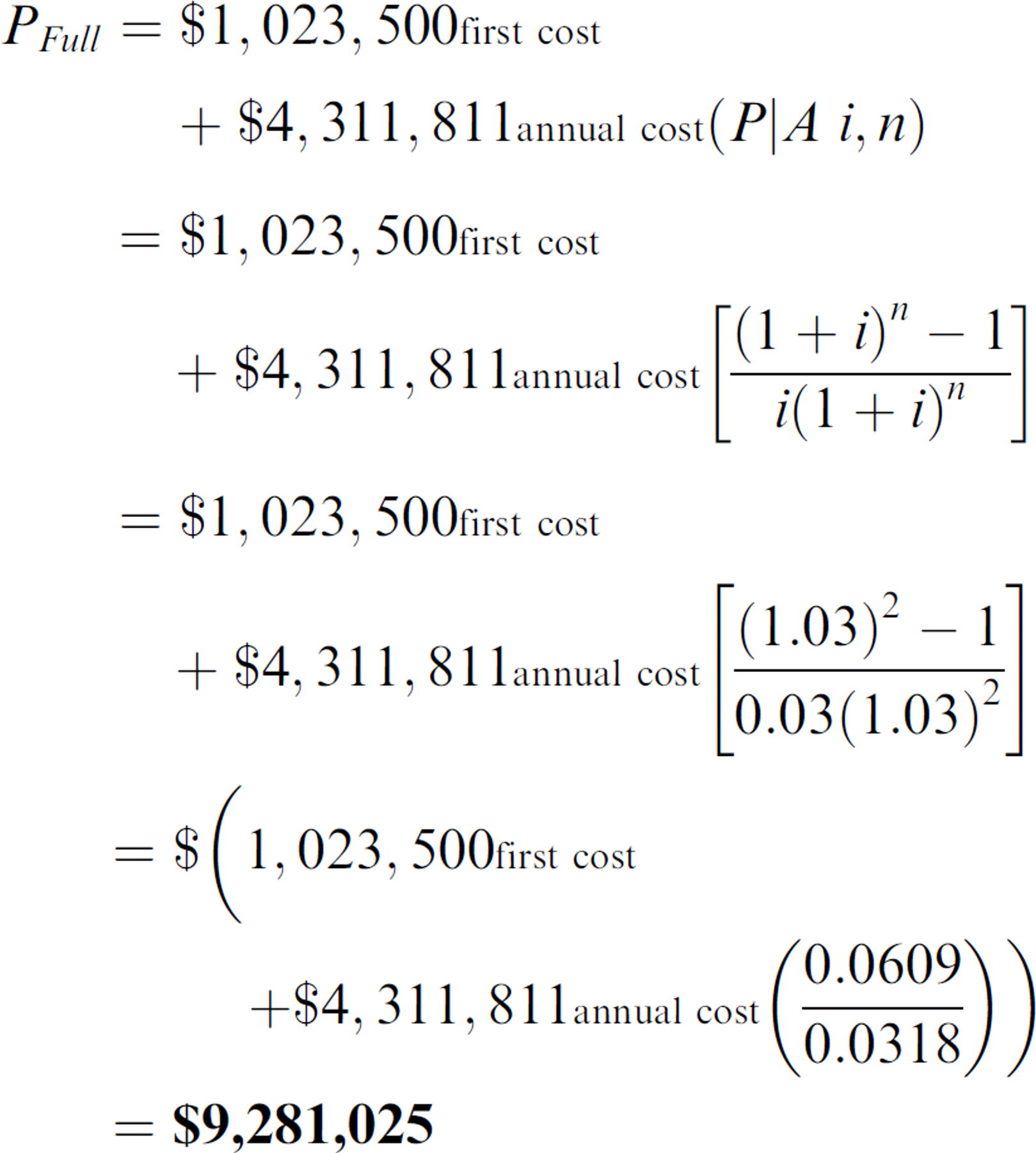
In the following, we solve for the present worth of the full automation alternative.

$\begin{array}{c}{P}_{\text{Full}}=\$1,023,{500}_{\text{first}\hspace{0.17em}\text{cost}}\\ +\$4,311,{811}_{\text{annual}\hspace{0.17em}\text{cost}\left(PA\hspace{0.17em}i,n\right)}\\ =\$1,023,{500}_{\text{first}\hspace{0.17em}\text{cost}}\\ +\$4,311,{811}_{\text{annual}\hspace{0.17em}\text{cost}\left[\frac{{\left(1+i\right)}^n-1}{i{\left(1+i\right)}^n}\right]}\\ =\$1,023,{500}_{\text{first}\hspace{0.17em}\text{cost}}\\ +\$4,311,{811}_{\text{annualcost}}\left[\frac{{\left(1.03\right)}^2-1}{0.03{\left(1.03\right)}^2}\right]\end{array}\begin{array}{l}=\$(1,023,{500}_{\text{first}\hspace{0.17em}\text{cost}}\hfill \\ +\$4,311,{811}_{\text{annual}\hspace{0.17em}\text{cost}}\left(\frac{0.0609}{0.0318}\right))\hfill \\ =\$9,281,025\hfill \end{array}$

Figure 8.

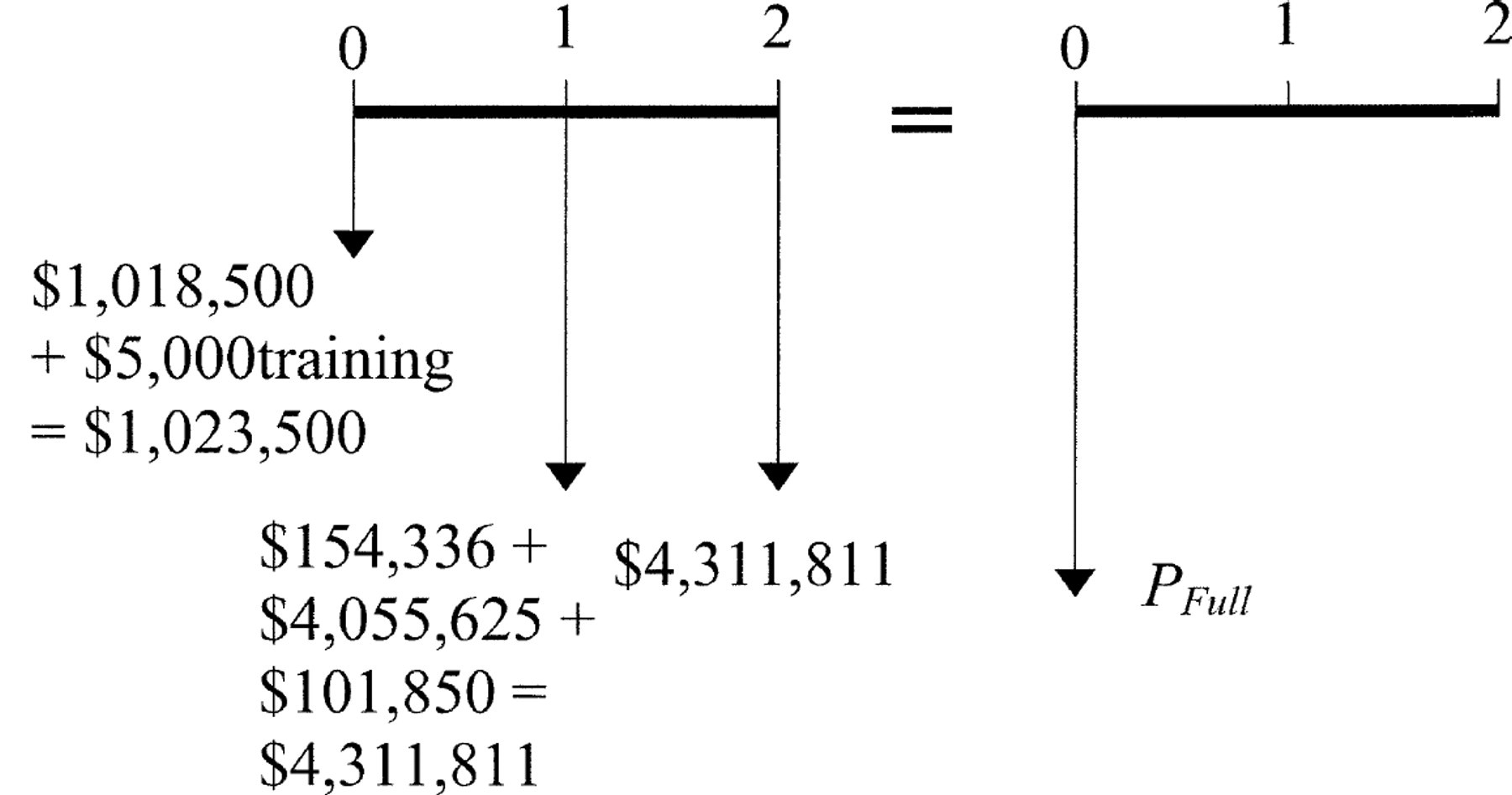
Cash flow diagram for the full automation method of example 9.

If the experiment is completed in one year, then we can calculate the following:

$\begin{array}{c}{P}_{Full\hspace{0.17em}}=\hspace{0.17em}\$(1,023,{500}_{\text{first}\hspace{0.17em}\text{cost}}\\ +\$4,311,{811}_{\text{annual}\hspace{0.17em}\text{cost}}{\left(1.03\right)}^{-1})\\ =\$5,209,729\end{array}$

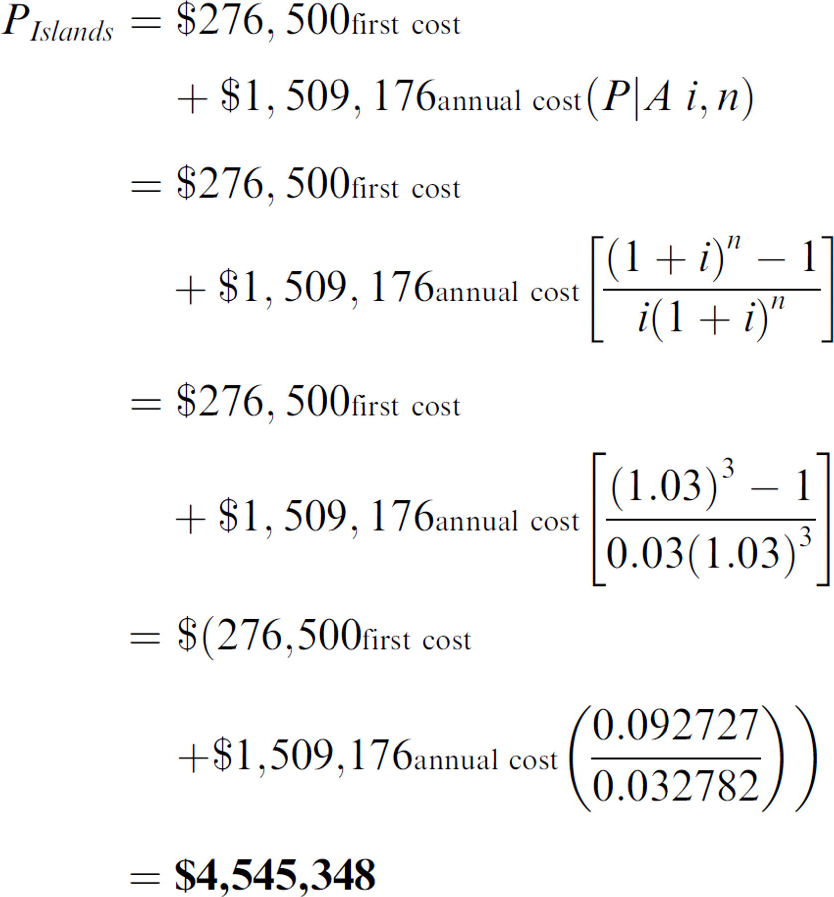
The results of this example show that islands of automation/workstation-based automation alternative is the most cost-effective approach with a present worth of $4,545,348, as compared to $5,467,768 for the manual alternative and $9,281,025 for the completely integrated full automation alternative. Although the upfront costs for the manual method initially are lower than for the islands of automation, the annual costs are higher and are further magnified by the effect of compounding over 3 years. It is interesting to note that if the full automation alternative could meet the throughput goals to complete the tests in one year, then it would move to second place, with a present worth of $5,209,729.

It is here that unquantifiable costs come into play because it is difficult to assign a cost or a value to the amount of time required to complete an initiative. It often comes down to a judgment call based on how a company perceives its sense of urgency for a particular initiative. Unquantifiable are issues such as user acceptance, flexibility, and marketing concerns. Full automation can look very impressive, although, by itself, this is not a good reason and should not be weighted too heavily. If assays change relatively frequently, or if a company wishes to have lab technicians run equipment, then it is likely that islands of automation will be more cost effective because it is easier to train technicians and to modify equipment operation. If time is the most critical issue, then full automation is usually the preferred solution. But, performing an economic analysis is still necessary to verify the conclusion.