Concepts for Dynamic Scheduling in the Laboratory

Abstract

Laboratory environments are controlled more and more by automated systems. Written procedures and lab journals are replaced by workflow description languages and electronic notebooks, which not only describe the processes but are used also for the control of the entire workbench, data acquisition, and documentation. Dynamic scheduling is needed in such an environment. Multiple samples with different procedures are processed in parallel, competing for the instruments. The whole environment may be also underlaid by optimization strategies like throughput or minimum sample processing time.

The modeling of all components interacting on the workbench—samples, devices, sensors, results, database systems, and so on—needs to rely on concepts building a consistent framework. This article gives a set of terms and definitions used in a dynamic scheduling environment. It describes most of these entities in detail, including their functionality and attributes as well as their logical and physical interactions. It also describes concepts such as workflows with activities and constraints, functional libraries, hidden transport, and dynamic execution. Maintenance, calibration, and error management also are included. Finally, it discusses how the entities interact with the different components in the scheduling system.

Introduction

Workflows in the laboratory range from high-throughput screening tests, in which many different samples are processed by using the same procedure, to a quality control (QC) environment with a great variety of different products and different workflows. Sample preparation and testing steps within a workflow—the activities—are executed on analytical instruments and sample handling tools. Different activities for different samples compete for these devices. The use of scheduling algorithms is required to determine the execution sequence for the various activities, as well the corresponding use of resources. A number of conflict detection and resolution strategies are employed to find an optimal working plan for the jobs to be processed on the laboratory workbench.

A set of concepts describing the processes needs to be defined to implement a proper scheduling system. These concepts include devices, different types of activities, the composition of activities and procedural elements of workflows, as well as the ability to record result and sensor data. Their storage and retrieval are discussed in this report. The features that influence the process, depending on information gathered at run time, are also covered, as is the notion of run-time variables and their implications for remaining system components. In addition, functionalities for synchronizing activities and workflows (e.g., for calibration) and managing maintenance are addressed, and the results, calculation, and documentation steps are presented.

The concepts described in this article were developed as part of a larger project to create a configurable dynamic scheduler that can serve both in a laboratory and in semiconductor production.

Fundamental Requirements and Concepts for Scheduling

Terms and Definitions

Activity . An activity is an element of a workflow defined by an end user. It is defined by its duration and constraints to other activities. It may consist of several working-plan activities.

Analytical procedure . An analytical procedure is a set of sample preparation operations and tests that are performed to verify a product's quality. In a laboratory, analytical instruments are used to measure physical or chemical parameters.

Capability . A capability is an atomic attribute or atomic behavior of a device. It may disappear after a certain number of operations or a predefined duration. A calibration or maintenance workflow may restore the capability.

Device . A device is a physical instrument on a workbench that has one or more capabilities. It is an example of a device type and can be a sensor or an actuator. Pseudodevices may be used to execute storage and retrieval tasks on computers or to calculate mathematical expressions. Devices and pseudodevices are accessed via an application programming interface.

Device adaptor . A device adaptor is a program that allows a physical device to be remotely controlled through software.

Device group . A device group is a set of physical devices with one or more identical capabilities. A device group may consist of physical devices belonging to different device types.

Device type . A device type is a class of devices with identical capabilities. All devices of the same device type can be treated interchangeably. Each of them can be used to perform a specific activity.

Dynamic scheduling . Dynamic scheduling is a process that creates a resource-specific working plan that is based on a set of activities belonging to identical or different workflows. This working plan is monitored and adapted at run time to react to system or user events, such as ad hoc samples or workbench exceptions.

Dynamic scheduling needs to include remaining working plans into its scheduling algorithms.

Macro . A macro is a working plan that is composed of activities and procedural workflow elements.

Optimization criteria . Criteria that influence the selection of working plan alternatives. Optimization criteria are calculated by the scheduling algorithm. Examples include maximum sample throughput, minimum sample processing duration, and minimum reagent consumption.

Flow control element . Flow control elements are used to perform count loops, while and until loops, conditional branching, and concurrent operations.

Remaining working plan . A remaining working plan is a working plan that has not yet been processed or that has been processed only partially. It may contain activities that are scheduled on unavailable instruments.

Scheduling algorithm . A scheduling algorithm is a sequence of mathematical operations that assembles and optimizes a working plan from the given activities and workflows. It allocates processing time on devices. In addition, it considers any sample- or workflow-specific constraints as well as global optimization criteria when making placement decisions.

Static scheduling . Static scheduling is a process that creates a fixed resource-specific working plan based on a set of activities belonging to identical or different workflows. The resulting working plan cannot be modified at run time.

Time constraint by mutual boundaries (TCMB) . A TCMB is the constraint between the start or finish time of an activity and the start or finish time of another activity. At each end of a TCMB, a number represents the boundaries of the activity time on the other side of the TCMB constraint.

Time-bounded sequence . A collection of time-constrained, connected activities with a common start and finish form a time-bounded sequence (TBS). TBSs may be expressed by TCMBs.

Workflow . A workflow is a sequence or graph of activities, macros, or special activities that are connected by time constraints or conditional constraints. Activities in a workflow may be bound to either device types or particular devices. A workflow can have local variables, which can be accessed and manipulated by its member activities. Parameters can be used to pass variables between workflows.

Workflow element . Workflow elements are elements of the workflow description language. They are divided into two groups: (1) activities, macros, and special activities (e.g., split and merge) and (2) flow control elements.

Working plan . A working plan is a set of working-plan activities that are executed on different devices. It is generated by the scheduling algorithm. A Gantt chart may be used to represent it graphically.

Working-plan activity . A working-plan activity is an atomic element of the working plan that is executed on a real or pseudodevice (see the Resources section of this article).

Background

Scheduling in a multidevice environment is required in many industries. Products are often manufactured on assembly lines, for example, car assembling, consumer electronics assembling, pharmaceutical production, or continuous processes such as petroleum refining.

Laboratories also need scheduling. Samples with analytical procedures are processed on workbenches in parallel or sequential order. Here, multiple samples and procedures compete for the same devices. Through the use of specific conflict resolution strategies, resources can be shared, and throughput can be optimized. Optimization strategies can help reduce reagent and labor cost.

Figure 1 shows a schematic scheduling process. At first, the sample handling and processing is modeled as an abstract workflow. This workflow generically describes the individual processing steps for the sample. It covers the typical steps: sample preparation including capping and decapping of containers, weighing, shaking, diluting, and sealing. A workflow may also contain run-time calculations that use variables and database operations. To shield the end user from the peculiarities of the workflow description language, it may be manipulated by using a graphical user interface. Here, activities and flow control operators can be arranged on a drawing board by using drag-and-drop operations. Details may be added by double-clicking on the icons. A subsequent pop-up dialog then accepts all necessary parameters.

Figure 1.

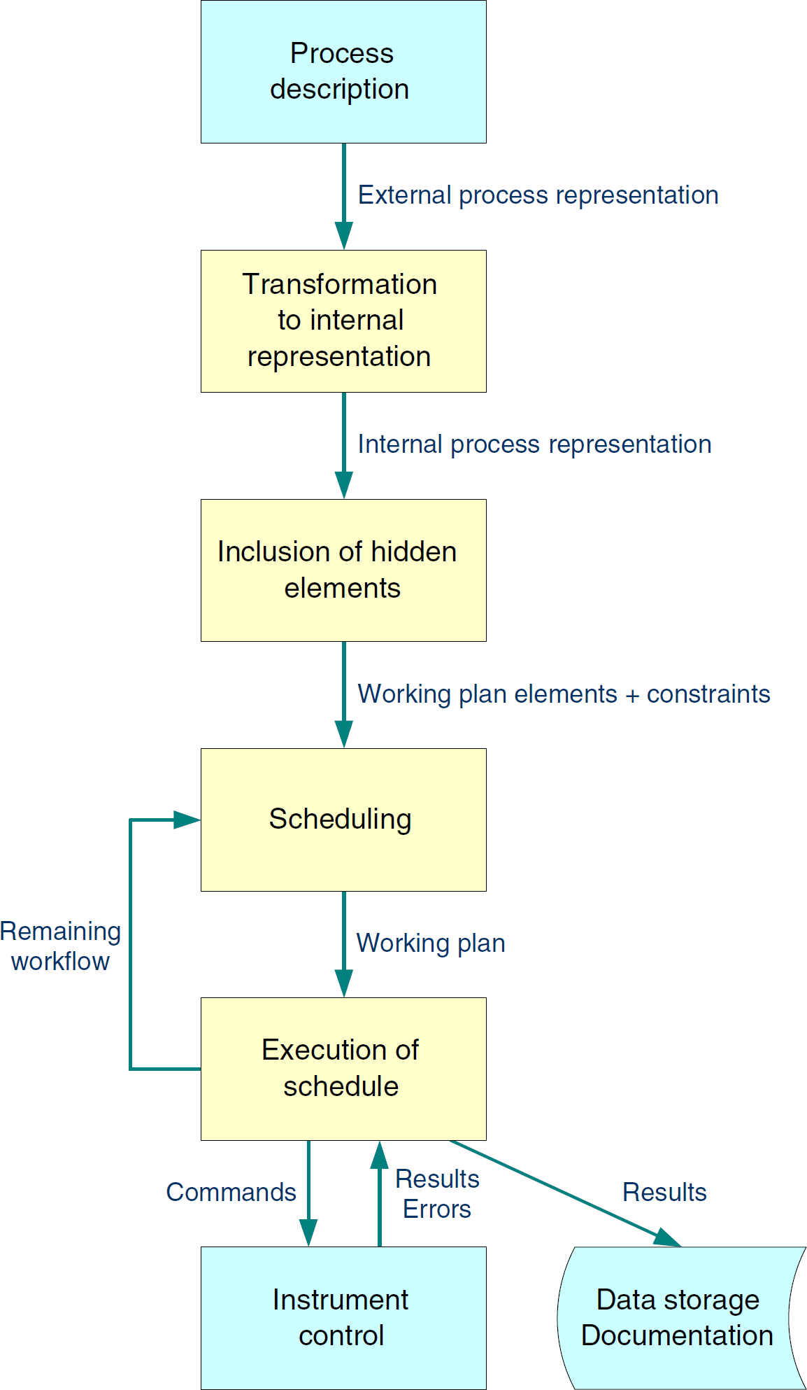
Schematic flow in a scheduling system.

The scheduling system can provide a number of features to improve user experience. One of them is the hiding of sample transportation steps. Because the system is aware of the locations of all samples and devices on the workbench, it can generate the appropriate robotic movements automatically. This allows an end user to focus on the chemistry and biology of the experiment, rather than on automation issues.

To process a particular sample, an end user picks one of the analytical methods that have previously been defined as workflows. This means that a workflow is instantiated for the sample. The system uses the workflow definition to calculate a working plan with the scheduling algorithm. The algorithm selects suitable devices to perform the processing by matching the capabilities needed by the activities with the capabilities provided by the individual devices. Time and conditional constraints, sample priorities, device downtimes, calibration and maintenance cycles, and so on also are taken into account. To find a (close to) optimal working plan, multiple plans are calculated and evaluated in relation to the user-specified optimization criteria. The final working plan is subsequently transferred to the executor, a component that is responsible for sending commands to the devices controlling the timing and detection of timeouts. It also acquires the measurement results, checks their tolerances, and transfers them to their final storage locations. The executor can control multiple devices in parallel. It also manages the user-defined run-time workflow variables.

In case of device outages or other serious workbench events, it may not be possible to complete the work as scheduled. In such cases, the executor notifies all other components and instructs the Scheduler to recalculate the remaining part of the working plan.

Resources

Physical devices . Physical devices are analytical instruments (e.g., balances, high-pressure liquid chromatography [HPLC] or gas chromatography [GC] devices, photometers, NMR spectrometers), sample preparation devices (e.g., pipettors, cappers, sealers, labelers), or handling systems (e.g., robots, rail transporting devices) that actually exist on the laboratory workbench. In addition, there are automated material input ports, photoelectric barriers, and command-finished buttons to notify the system that the user accomplished his manual task. Physical devices are controlled by the executor with an instrument-specific device adaptor.

These devices are driven by commands stored in a system capability data set. ¹ This repository also contains the geometry of the device and its material ports, as well as calibration and maintenance information. It may also store workflows needed to resolve error conditions.

Pseudodevices . Chemical processes often involve calculation and information-handling steps. These can be modeled with pseudodevices. Pseudodevices do not have a physical equivalent on the workbench. Instead, their functionality is provided by a software component inside their device adaptor. For example, interfacing with an SQL database is solved by using a pseudodevice. The database driver is treated as a device adaptor to the database pseudodevice.

Calculations can also be handled by using a so-called calculator pseudodevice (see the Concept of variables paragraph in the Requirements for a Workflow Description Language section ahead).

Like physical devices, pseudodevices can have error conditions. They also can use workflow variables to exchange data with other workflow elements.

Multiposition devices . On a multiposition device, several samples may be processed at the same time under the same conditions. For example, on a shaking device, processes using this feature can run very efficiently.

For example, consider a shaking device: sample A must be shaken for 10 minutes at 100 rpm, sample B for 20 minutes at 100 rpm, and sample C for 30 minutes at 100 rpm. The sequential manual process requires a total of 60 minutes. An automated process needs only little more than 30 minutes: Place all samples on the shaker. After 10 minutes, remove sample A, and so on. In this example, this operation saves approximately 50% of the execution time.

An HPLC sampler is another example for a multiposition device. During the injection of a sample, a robot may unload or load other samples at different rotor positions. Here, the overall sample loading performance may be improved.

Supporting multiposition devices appropriately promises significant throughput improvements. In some cases, using such a feature will not work, because the activity needs to be interrupted when samples are added to or removed from the process. This may not be feasible in certain cases.

Consumables and durables . Consumables (e.g., reagents or indicators) may be treated as one of two cases: (1) as resources that are infinitely available or (2) as samples. Case 1 implies that the availability will be controlled externally to the system, whereas in case 2, the availability control may be included as part of the resource control mechanisms. Merge operations are used to apply consumables to samples. In these steps, the consumables' sample ID will be discontinued, and the original sample's ID will identify the material after the merge.

Containers . Containers are used to carry material on the workbench. They may be anonymous and processed without their own ID. In this case, the material ID becomes the container identification.

On the other hand, a container feeder may deliver uniquely identified containers for subsamples. In this case, the subsamples carry the container IDs as unique sample IDs as soon as the sample material is added to containers. The transfer of the ID either may be done explicitly in the workflow by using workflow elements or may be hidden in a sample split workflow element.

Activities

Basic activity concepts . The definition of activities and their attributes are essential for the development of scheduling systems. They belong to the core functionality. The device command is the major element in an activity. Activities refer to capabilities needed to execute a process. Normally, capabilities are not bound to special devices. It is only in special cases that specific devices may be addressed in an activity. The command is sent to the device in the execution phase.

For example, the physical equivalent for the logical command READ (balance A, weight) is sent to the balance instance A. The result is handed over to the variable weight, which then may be used to check the tolerance in a subsequent working-plan activity.

Manual activities may also be included in a workflow. It is essential to allocate enough time for their execution. As a specialty, an activity-finished event generator (e.g., a pushbutton) can be added to allow an operator to indicate the conclusion of the activity.

Fig. 2 shows the parameters of an activity. Because the duration of a chemical process never can be predicted exactly, the user mostly uses a supremum of durations, d_max (see Fig. 2a). Process conditions may limit the activity to a minimum duration d_min (see Fig. 2b). In special cases, the subsequent activity must not start later than a predefined maximum delay, Delay_max, after the activity's end. The delay might also feature a lower limit Delay_min. During an activity's execution, only the actual duration d_actual will be employed (see Fig. 2c).

Figure 2.

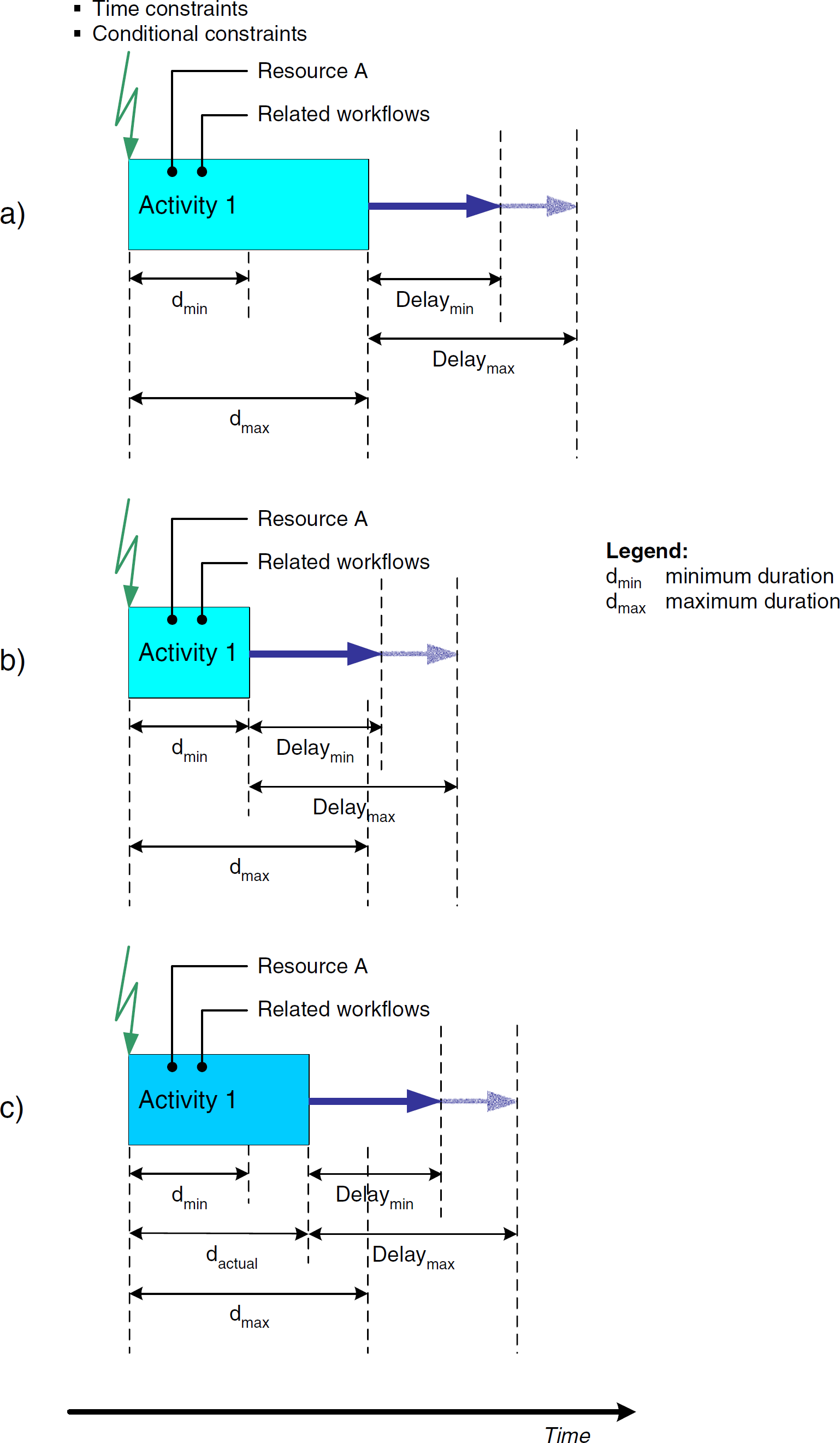
Definition of activities.

The activity has predecessors triggered via time and conditional constraints. An activity may also generate triggers for subsequent activities (see the Relationship between working-plan activities and device allocation implication section, next). They are normally transferred via variables (see the Requirements for a Workflow Description Language section ahead).

An activity can use a device, containers, consumables, and durables. All these resources are accessible via variables.

Error handling is also built into working-plan activities. Classified exception reaction workflows are specified explicitly in each activity. They should be defined in an error workflow that is triggered via a special error exit mechanism. The main objective is to keep the workflow almost entirely free for the chemical process.

Relationship between working-plan activities and device allocation implications . Activities are connected via time and conditional constraints (see Fig. 3a). They are normally arranged in end-to-start order; that is, the subsequent activity starts after the first activity is finished. Even if the first activity normally ends earlier than d_max, the resource connected to it needs to be allocated for the activity's maximum duration (Fig. 3c). Note that the actual resource allocation may also be as short as d_min (Fig. 3b). The working plan may also imply that the sample has to be parked on the device until the next activity starts. In this case (Fig. 3d), the reservation times on the instruments might even be longer, and the reservation times of subsequent activities might overlap. For exact times, refer to the annotations in Fig. 3.

Figure 3.

End-to-start relation between activities including device allocation.

Activities may also be started at the same time, such as in the case of samples on a shaking device (Fig. 4a; start-to-start relationship). In a workflow, this might be modeled by using the TCMBs.

Figure 4.

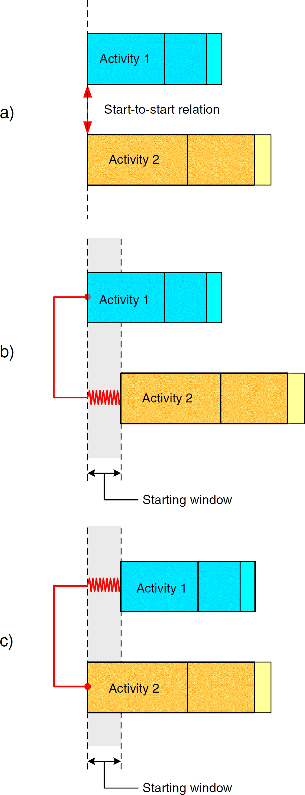
Start-to-start relation between activities.

Fig. 4b shows another situation in which activity 1 begins execution and activity 2 follows shortly before the time window is finished, for example, adding a reagent to a sample shaken in parallel. The spring indicates that the real starting time of activity 2 also may be earlier. The scheduling algorithm has the freedom to select any starting time within the window. Fig. 4c shows the contrary situation: activity 2 starts before activity 1. Both situations should be definable in a workflow editor, knowing that a chemical process's timing in most cases is not as exact as, for example, assembling processes in the semiconductor industry.

The TCMB metaphor even allows modeling the variability of delays between activities. With this feature, the scheduling algorithm can automatically minimize inactivity times of devices.

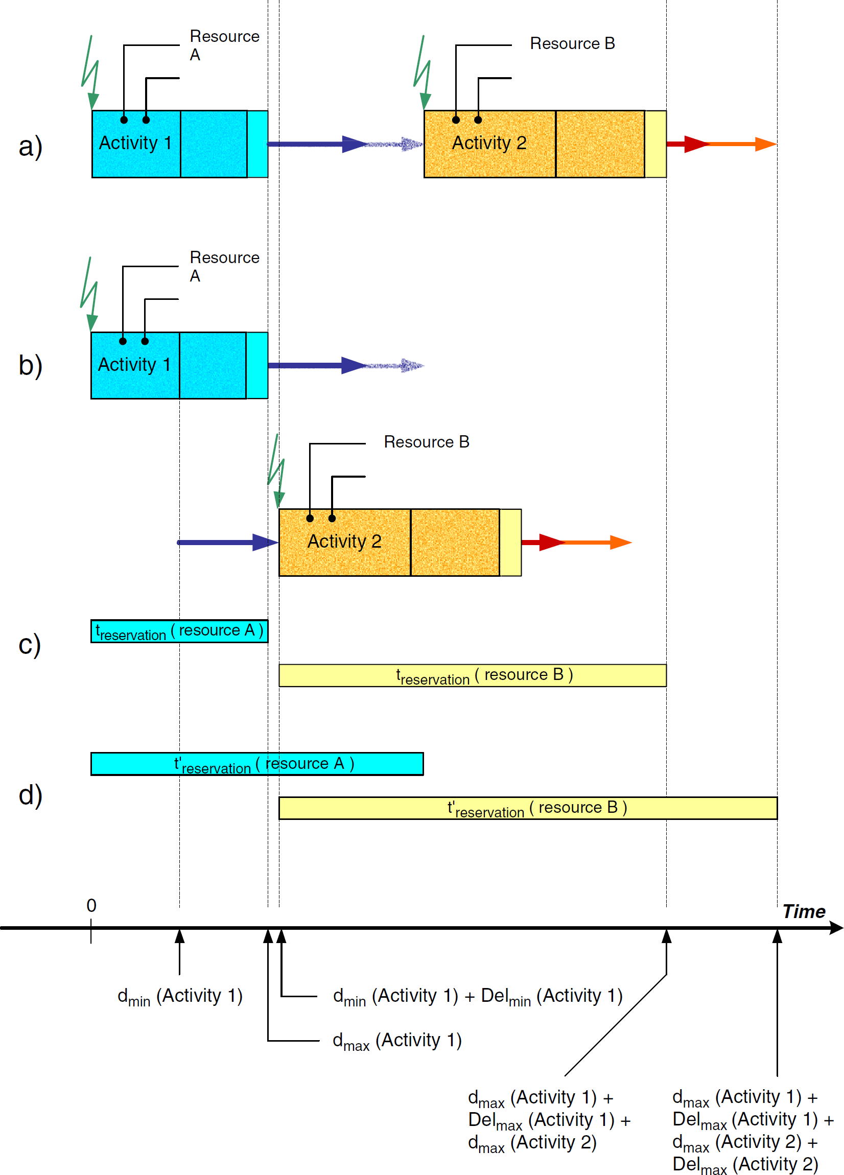
Modeling becomes more complex in end-to-end relations of activities (Fig. 5). Fig. 5a visualizes the situation at workflow definition time. d_max(Activity 1) and d_max(Activity 2) are used to define the end-to-end relation. However, the end of activity 1 is flexible; that is, activity 1 will end at d_actual, where d_min ≤d_actual ≤d_max. This means that even if an end-to-end relation is specified between both activities, the system will use dactual(Activity 1) and dactual(Activity 2) during execution.

Figure 5.

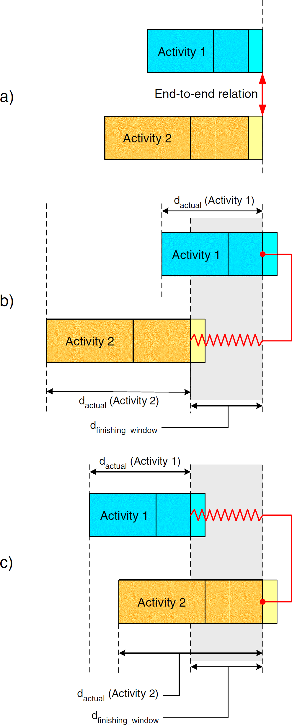
End-to-end relation between activities.

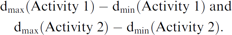
An interesting situation can be seen by looking at a device's reservation times and the finishing window duration d_{finishing_window}. Looking at Figs. 5b and 5c, it is easy to understand that d_{finishing_window} equals the longer time difference of the following:

$\begin{array}{c}{\text{d}}_{max}\left(\text{Activity}\hspace{0.17em}1\right)-{\text{d}}_{min}\left(\text{Activity}\hspace{0.17em}1\right)\hspace{0.17em}\text{and}\\ {\text{d}}_{max}\left(\text{Activity}\hspace{0.17em}2\right)-{\text{d}}_{min}\left(\text{Activity}\hspace{0.17em}2\right).\end{array}$

In the example, it is the difference belonging to activity 2. The two cases depicted in Fig. 5b and 5c show that the spring behind the activities allows a flexible end within the predefined interval.

The devices' reservation time results in d_max(Activity 1) + d_{finishing_window} and d_max(Activity 2) + d_{finishing_window}.

Delays do not have to be limited. They may have a lower limit Delay_min, but the upper limit may be infinite (Fig. 6). In this case, a major advantage results. The scheduling algorithm may squeeze as many different sample activities into the gap between activity 1 and 2 as possible. Subsequently, the working plan reflects an optimal working plan timing regarding the optimization criteria.

Figure 6.

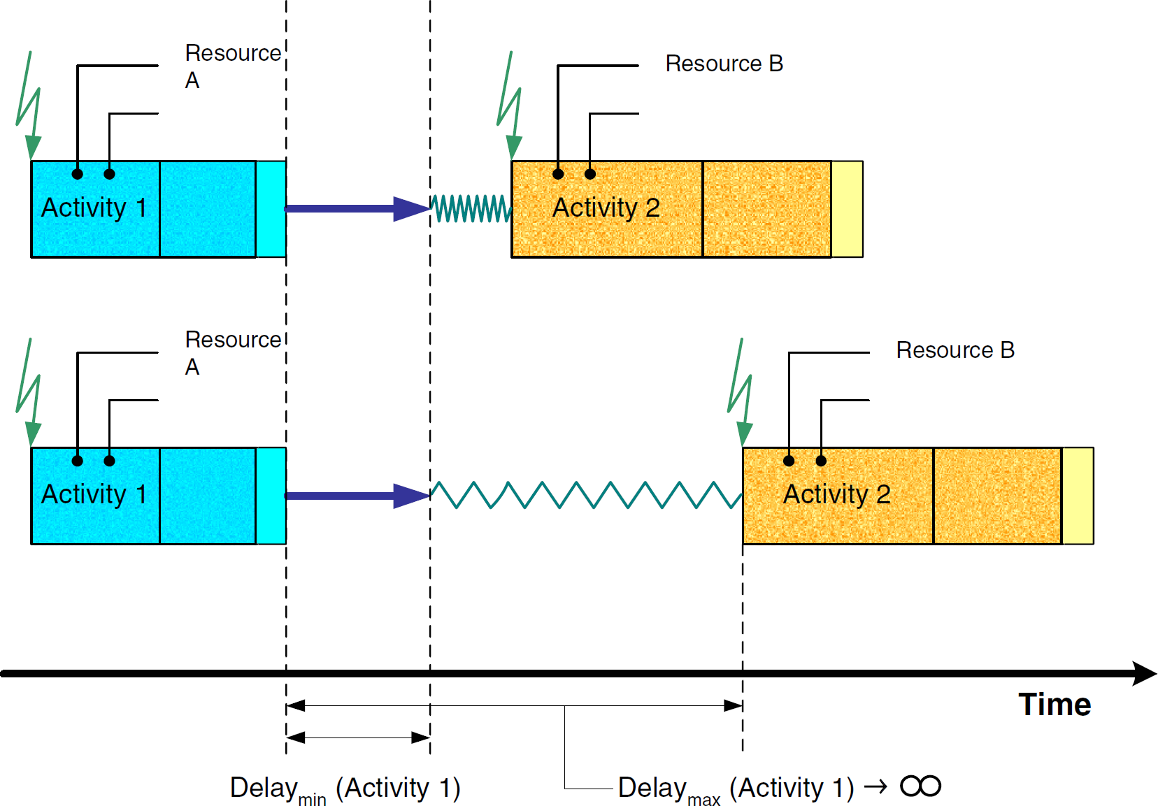
Infinite delays between activities.

Time-bounded sequences . Restricted times over a series of activities are TBSs. They occur relatively often in a laboratory. For example, consider an incubation step immediately followed by a testing step. TBSs are modeled with TCMBs. The TCMB spans all activities between the first and last activity belonging to the TBS. In this incubation example, the TCMB starts directly with d_max(Activity 1) and ends with the beginning of the testing activity.

The scheduling algorithm must not break such a TBS time constraint, which means that the scheduled TBS duration must be shorter than or equal to the TBS duration in the workflow. The algorithm may insert activities belonging to other samples between TBC activities if the duration of one or more gaps is sufficient.

Data-handling capabilities . Taking care of result data and controlling the process in real time with sensors is an absolute necessity in an automated laboratory. The workflow does not consist only of device control. Results and their arithmetic manipulation, storage, and retrieval need to be included in workflows.

Arithmetic functionality may be provided via a pseudoinstrument. Data elements hold variables for the basic operations (see Concept of variables paragraph in Requirements for a Workflow Description Language section ahead), which are evaluated by an interpreter. Functions are accessed via function calls with parameters; for example, ADD(a,b,c), which is equivalent to c = a + b in algebraic notation. Such function calls correlate to device commands, such as READOUT(resultString). Different calculation operations are activated by different function calls.

Data storage also is modeled by a pseudodevice. Its commands control SQL-like functions for select, insert, update, and delete. Storage locations in the database tables are addressed via variables containing values for their primary keys. Variables are used to transfer results back and forth. There even might be a construct for direct and indirect addressing, for which direct addressing would allow for carrying result values directly. In indirect addressing, on the other hand, only the storage location containing the results would be referenced.

The concept of data handling implies that data can be directly included into decisions or calculations. For example, a proof-of-specification test may be integrated into a workflow, thus making its result directly available for decisions in subsequent working-plan activities.

Sample split and merge . Many experiments in a laboratory require sample split and merge operations. Sample splitting occurs in replication operations (e.g., within a sample bank or during sample fractioning). An original sample is split into derivative samples. There are situations in which the number is known during workflow specification (case 1: sample bank with normal sample split). On the other hand, there are also scenarios in which the number of derivatives may not be known before the execution of the experiment (case 2: Sample fractioning).

In case 1, the scheduling algorithms easily can extract the number of derivate samples from the workflow and provide the adequate resource allocation for their execution. The naming convention for the derivative samples could be based on a parent-child or subindexing scheme, such as the following:

$\text{original}\_\text{sample}\_\text{ID}.\text{derivative}\_\text{sample}\_\text{ID}$

Compared with case 1, case 2 is more complicated because there exists no a priori knowledge of how many subsamples (and time slots) have to be allocated during scheduling. Subsequently, the scheduling algorithm cannot define the starting time of the activity after the fractioning step. It will be in the remote future during the execution phase; thus, the only solution in this case is to ask the user at workflow specification time to provide a good estimate of the number of derivative samples. The scheduling algorithm applies this number to allocate the execution slots. The workflow has to include a last-fraction check in each loop. The executor then processes this loop with the checks for completion. The loop is terminated as soon as all fractions are processed.

Sample merge operations, for example, are needed for adding internal standards or reagents to the sample being tested. The identification of the resulting material is based on the sample's original ID. A process to assign the resulting ID must be provided by the system.

Macros

The workflow generation should be efficient to minimize the process definition steps for the user. A library concept supports this functionality. The user may compile a number of generic workflow building blocks (macros) that can be applied to many situations. These macros can be stored in a library. Depending on the type of macro, a macro may require input parameters to customize its operation. Examples of typical macro input parameters are sample IDs, values for conditional branch decisions, sample weights, and so on. Macros may also return (output) parameters or return values for activities after the macro. In both situations, a parameter handover and marshalling mechanism must be provided. To simplify data handling within macros, the macro definition language should also provide a means for defining macro-internal or local variables.

Dynamic Execution

The scheduling algorithm calculates the timing in the working plan (i.e., the reservation times for the different devices). The working-plan activities on the different traces of the related Gantt chart hold all variables for duration and delays. In case of a fixed delay between two working-plan activities and d_actual(Activity 1)<d_max(Activity 1) (Fig. 3), the subsequent activity must be moved up to an earlier time slot (i.e., the execution of activity 2 must start earlier than originally planned for in the workflow). This effect is called dynamic execution. As a result, the reservation time for working-plan activity 2 is longer than its maximum duration d_max and needs to start earlier than its scheduled starting time.

Visible vs. Hidden Activities

Activities need to be defined carefully. At a minimum, the following two alternatives may occur:

Activities are defined in the finest granularity. In this case, an activity always represents one command sent to one device. In this case, an activity is identical to a working-plan activity. This first case is called working-plan activities only.

The activity definition is in a higher granularity. Here, an activity consists of several working-plan activities. However, the semantics of these working-plan activities remains the same. This second case is called working-plan activities with fine structure.

The case working-plan activities with fine structure implies that the fine structure of the activities is hidden. As a result, a mechanism for adding these hidden structures in the transition from the external representation of the workflow to the executable working plan has to be provided. The complexity of this mechanism is very high.

The working plan depends highly on having access to the complete fine granular working-plan activity information. This leads to clear workflows in which most activities represent the chemical process.

In the case of working-plan activities only, the chemical process is not reader friendly, because it is covered by control working-plan activities.

Fig. 7 illustrates a detailed activity breakdown structure. The different traces in the Gantt chart show the activity's fine structure.

Figure 7.

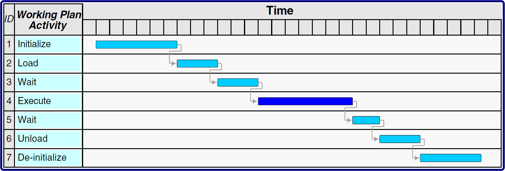
Fine granularity of an activity.

Example: An activity can be initialized with a series of commands, such as move to the gripper magazine, execute the macro change gripper, and move to the sample location. The Initialization step of a robot is never linked to a sample. In the Load working-plan activity, the robot grabs the sample. The subsequent Wait step is not being used in this example. In the Execute step, the robot moves the sample to the next device. The adjacent command takes as an argument the actual robot position as the starting point of the trajectory and the target device location as the trajectory's end point. The second Wait step is not used in this example either. In the Unload phase, the robot's gripper releases the sample. Finally, the robot optionally unloads the gripper in the Deinitialize phase. All working-plan activities except Execute are optional.

In the case of analytical devices such as multiposition devices, the first Wait phase is necessary to pause all samples already on the device during the next sample loading. The second Wait step usually is used during the unloading of multiposition devices.

A robotic motion activity is even more complex. Given that certain material ports of an instrument may not be approachable from all directions, a relatively simple trajectory (path) planning concept similar to the ones used in avionics might be applied. For example, the robot first moves from its current or home position to the trajectory starting point. After that, the device's automatic-landing system and obstacle avoidance algorithm guides the robot to its trajectory's touchdown point in 3-D space. All these robotic moves have to be incorporated into the instrument-specific workflows to be automatically included into workflow expansions. Knowing that the sequence of the different samples' activities (including the locations of their device instances) is arranged by the scheduling algorithm, manual inclusion of such kinematics is not feasible.

Please note that there is a close relation between two subsequent activities: the first one is executed on a normal analytical device (e.g., a balance) and the second is executed on a transport system. This example would require the Unload of the balance to make reservation of the balance, although it is inactive during this time interval. The robot's Load (i.e., “grip sample”) command is active during this interval. It follows that there must be a start-to-start and an end-to-end time constraint between both the balance's Unload and the robot's Load working-plan activities.

In case of several instances of the same balance type, for example the Sartorius “GENIUS ME235P,” the different device locations must be considered. These locations cannot be included until the algorithm selects the specific balance instance. Therefore, it is obvious that the user wants only to write down the execution phase of an activity with the device type (see Background). The software should be able to include the remaining details automatically, without user intervention (Fig. 2).

This also demonstrates that the working plan must be much more detailed than the workflow to be able to drive the workbench.

Finally, it is important to consider device reservation times in the workflow. The Gantt chart in Fig. 8 shows an excerpt of a workflow, consisting of a sample weighing step and a subsequent GC content-of-active-ingredient test. The balance's working-plan activities are displayed in traces 1 to 7, the hidden sample transport is drawn in traces 8 to 14, and the GC's working-plan activities are shown in traces 15 to 21. The actual workflow's relevant working-plan activities are Balance: Readout in trace 4 and GC: Execute in trace 18.

Figure 8.

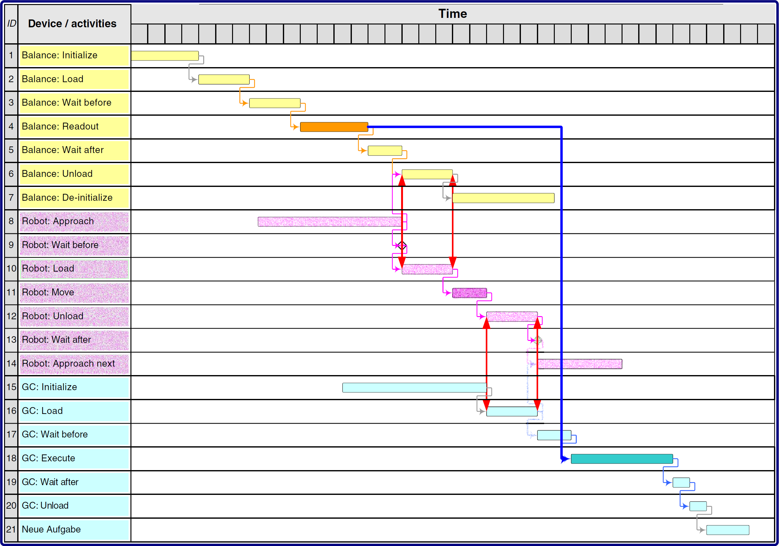
Hidden transport workflow example.

Inserting the hidden transport results is a relatively complex operation. First, the robot must be initialized (working_plan_activityID = 8; here, the approach of the robot with an empty gripper). Working-plan activity 9 is not needed. After that, the gripper takes the sample in the Load phase (ID=10), which must be synchronized with the balance's Unload (ID = 6). After the robot's Move, synchronization is made again between the robot and the GC (ID = 12 and 16).

Different device reservations overlap. The balance has to be allocated between the start of working-plan activity 1 and the end of working-plan activity 7, the robot between start of 8 and end of 14, and the GC between the start of working-plan activity 15 and the end of 21. It is important to note the overlap of the Load and Unload phases, which are located at the start and finish of the activities. Thus, the scheduling algorithm must work on the fine granularity to account for all time constraints.

Requirements for a Workflow Description Language

Control flow, data flow, material flow . The workflow primarily describes the sample control flow, but it must be parameterized to handle material, containers, consumables, and durables. The parameters are accessed via variables (see Concept of variables, next). Control, data, and material flow are different layers of the workflow. They are connected via variables whose values can be assigned and accessed through working-plan activities.

Concept of variables . Each workflow defines its own local variables, that is, variables with identical names in hierarchically structured workflows will be stored in different storage locations. Values may be assigned in one activity and accessed and used by another one. Variables may be transferred as parameters to macros or to other workflows by using a pass-by-value or pass-by-reference mechanism. There is a set of reserved variable names to allow for using information on a semantic level (e.g., sampleID, resultID, resultValue, workflowID, deviceID, and so on).

Fig. 9 shows the interactions and dependencies between the control flow and the data layer in a workflow. For example, in activity 2, a variable is assigned. Activity 4 then reads, computes, and saves the variable.

Figure 9.

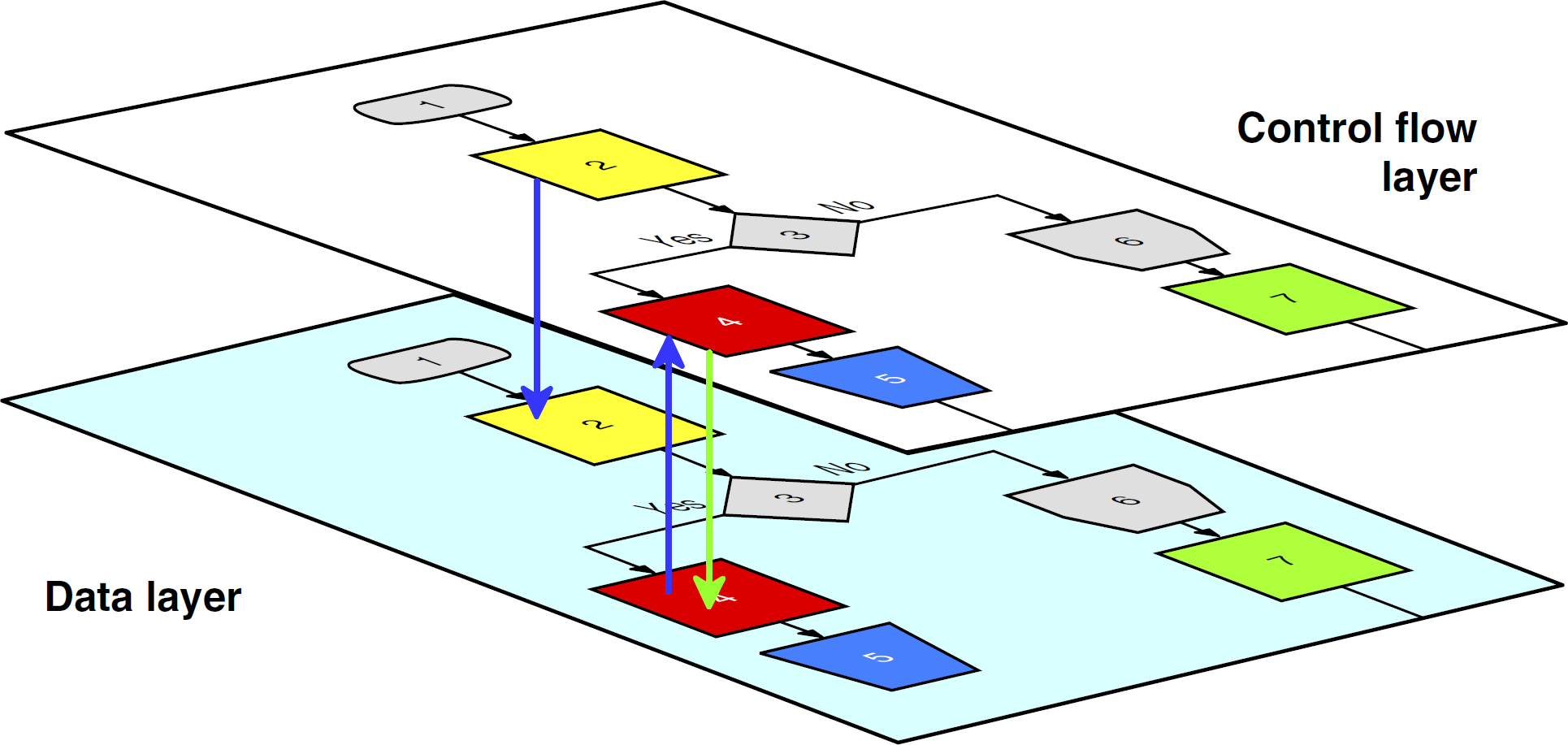
Control flow and data layer in a workflow.

Workflow elements . In addition to the activities, macros, and special activities described in previous sections, flow control operators are necessary to describe procedural interactions on a lab workbench. Count, while and until loops, conditional branching, and concurrent operations have to be provided to support more complex scenarios. As stated before, calculations and storage manipulations are also essential in the workflow. They are implemented via activities on pseudo devices. All workflow elements use the variable concept.

Most scheduling algorithms are not able to handle loop operations, especially not statistically unbounded loops such as while and until. Therefore, loops need special preparation steps before the scheduling. Loops are unrolled; that is, each cycle is inserted explicitly into the working-plan activity data structure. Unfortunately, the ending condition of while and until loops is not known before the process runs in reality. The process sets the condition. Without the ability to predict the number of cycles a priori, activity timing and device instances cannot be assigned to subsequent activities. As a result, the scheduling run cannot deliver a complete result. Consequently, while and until loops must be limited by the user. She or he must provide a maximum number of cycles for the algorithm to deliver a meaningful working plan.

Conditional branch operations should support the concept of branch probability (i.e., different branches may be executed with almost identical or very different probabilities). Given the fact that the user knows the probability of a branch ahead of time, the scheduling algorithm needs to make a reservation only for all devices on one branch. The branch with low probability can be neglected. If the low-probability branch will be needed at execution time, the working plan must be rescheduled. In case of almost identical probabilities, both branches are scheduled.

Concurrency on a workbench may be caused by (1) a split operation or (2) samples originating in the workflow. In case 1, all subsamples run in parallel, processing their predefined workflow steps. This may be a parallel physical operation if enough identical devices are present. If not, the scheduling algorithm can decide which branch should be executed first in accordance with optimization criteria.

Case 2 is more complex. One sample is processed in the workflow, resulting in the creation of another one (sample 2: external standard). Both samples are used for concentration testing in a double-beam spectrophotometer. The preparation of both samples is independent, but their partial workflows join before the concentration testing. The user indicates this by using a concurrent operation with the two streams included. The algorithm then can schedule the streams in accordance with optimization criteria.

Calibration and maintenance . Calibration and maintenance may be coded in normal workflows. But they must have additional properties compared with normal sample workflows. They are initialized and referenced in different ways.

Calibration has to be initiated in a predefined pattern, for example, every Monday morning at 7 am. The calibration is valid between two elements of this pattern. As soon as the calibration is overdue (i.e., the actual date and time belongs to the next interval in the pattern), test results are not valid.

Calibration results normally are accessed via activities connecting to a database. Activities performing a test on a specific device may branch to the calibration validation before execution. This check is implemented as a conditional trigger in the activity.

Maintenance may be handled in the same way as calibration. In addition, maintenance may also be necessary after execution of a prespecified number of activities on a device. For example, independent of the specific sample, the device may have to be cleaned after 10 runs. So, this mechanism is triggered by sample throughput. It is the job of the scheduling algorithm or one of its subcomponents to perform bookkeeping tasks such as activity occurrence counting. The activity may carry a condition such as check for number of maintenance events. If the number defined in the referenced device is reached, then the scheduler has to initiate a maintenance workflow before executing the triggered activity.

While undergoing maintenance, the respective device is not available for regular operations. Therefore, the scheduling algorithm must also take maintenance phases under consideration.

Master-detail workflow scenario . Today, enterprise-wide planning is practiced by many corporations. For example, a master plan for a production plant is set up to optimize the shop floor throughput. QC is one of the final steps in the production chain. The master plan is responsible for providing a timeline for QC operations to ensure proper load balancing among different laboratories with automated workbenches. One activity for a specific product's lot on the master plan is expanded into an entire workflow on the workbench level. Information about timing, available time buffers, lot size, workflows to be used, and so on, must be transferred from the master to the detail plan.

A similar situation may occur in a laboratory. For example, a workbench may reside at the master level, whereas an automated liquid handling station may be part of the detail level (Fig. 10).

Figure 10.

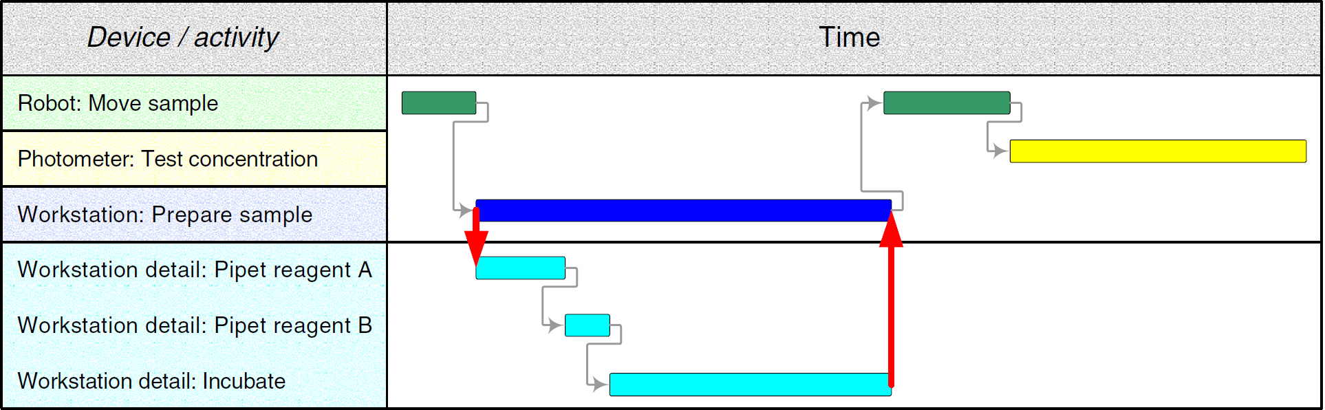
Master and detail working plans.

In both cases, input parameters must be propagated to the detail level and an accumulated result (e.g., lot conforms to specification) is returned to the master level.

In case of errors during the execution of the detail working plan, different scenarios must be taken into account. An error can imply that (1) the entire detail plan has to be canceled, (2) the detail working plan must start over from the beginning, (3) the detail working plan can recover on its own, and (4) the detail plan cannot recover on its own and the master plan has insufficient information to continue the process automatically.

These four cases indicate that a new kind of reaction may be in order. Case 1 needs a fatal error during execution of the detail working plan reaction. A parameter may notify the master level if the master activity can be rescheduled (case 1a) or not (case 1b). Case 1a triggers the reaction reschedule the lot on the master level. Case 1b triggers the standard reaction notify the operator. Both cases can be easily incorporated into an error workflow. All error codes must be linked manually into an error reaction workflow before the first use of the associated sample workflow. The mapping run time module may be implemented either on the detail or the master level. In both situations, the related information must be relayed from the detail to the master level.

Case 2 may be resolved by the detail executor automatically, but only if there is sufficient time left. In the case that automatic recovery is not feasible, the plan must be rescheduled at the master level. It is important to note that master level rescheduling is always followed by a detail level rescheduling (case 1a).

Case 3 implies the availability of a recovery workflow attached to the triggering detail activity. Case 4 must be manually resolved by the operator (see case 1b).

Implications for the Scheduling System Components

Workflow Implications

The workflow element's information structure allows implementing complex processes on the workbench. The workflow models the sample preparation, testing, result calculation, and data handling steps. Material transport, device initialization, calibration, maintenance, and error handling are reflected in the activity parameters. They are hidden in related service workflows. The end user (e.g., chemist) does not need to know how to implement and code them. She or he only needs to know their functionality and semantics. The actual implementation may be left to a system administrator or an automation specialist, who usually is most familiar with the intrinsic functionality of each workbench.

Workflows will be automatically expanded to their atomic granularity. Workflow elements and their constraints consist of all the information required for scheduling. The macros and service workflows are included in the right places. The workflow expansion produces a workflow tree, whose leaves represent the working-plan activities, including constraints. This tree can be used to monitor the samples on the workbench, even at the abstract workflow level (i.e., end-user level). The mapping of the low-level working plan information to the workflow can be achieved easily by traversing the tree from bottom to top (i.e., moving from the leaf nodes up to the root node).

Impact on the Scheduling Algorithms

The scheduling algorithm rearranges the sample-oriented workflow elements into the device-related working plan. By using constraints, priorities, device availabilities, multiposition device functionality, and so on, it calculates a working plan. Device types and device groups are replaced by real devices, that is, device instances. In addition, calibration and maintenance workflows have to be initiated because of their trigger conditions.

It is obvious that the different workflow elements and the working-plan activities imply special treatment in the scheduling algorithm. As stated previously, all loop operators have to be unrolled before calculation. Conditional branching requires special treatment. In case of almost identical branch probabilities, the algorithm has to allocate the devices in both branches (see Workflow elements paragraph in the Requirements for a Workflow Description Language section).

The optimization of the working plan implies a repeated application of the algorithm with different initial conditions. The algorithm's calculation time, including its optimization cycles, is crucial for good run-time performance. The algorithm must complete its run before the synchronization point between the current and the new working plan. If this condition fails (i.e., the recalculation takes too long), the new working plan becomes invalid, so the estimate requires sufficient buffers.

Scheduling algorithms are not discussed in this report. Readers may refer to the manifold literature, especially in the production environment. An in-depth, theoretical treatment of scheduling algorithms can be found in Brucker. ²

Implications for the Working-Plan Execution

The executor is responsible for processing the working plan. It simultaneously controls the devices on the workbench. In particular, it sends the commands, waits for returning results and status information, and accepts error messages. The executor also routes results to the correct destination to allow for calculation, storage, and retrieval operations. One essential executor task is the dynamic working-plan execution (see Dynamic Execution section).

The execution of commands is monitored continuously. If the command finished event is not generated on time, a timeout event is generated and is propagated to the system level. In this case, the executor has to generate a snapshot of the actual situation on the workbench and store it in the remaining working plan. Working-plan activities on the unresponsive (or potentially defective) device and their subsequent operations must be stored separately for rescheduling. It is important to consider that unrelated working-plan activities (e.g., activities belonging to different samples being processed on different devices) at the time of an error also may be affected. They may have to be rescheduled on the defective device at a later time.

The executor has to continue processing on all device traces not involved with the error. It also has to start activities that will be finished before the plan synchronization. TBSs may even end later than the synchronization point if they are not involved in the defective trace. Such working-plan activities must be handed over to the rescheduling process.

Exception Handling

Complex automated systems as described herein usually require fairly sophisticated error and exception handling to minimize system downtimes. This report addresses only the user's ad hoc involvement and errors generated by the workbench (Fig. 11).

Figure 11.

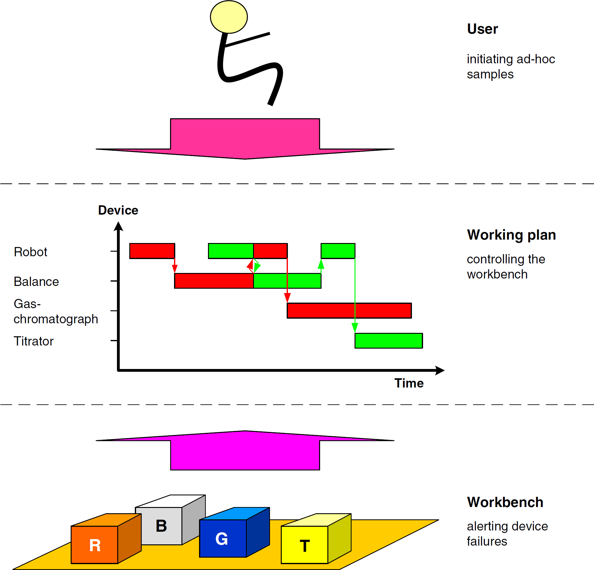
Events causing rescheduling.

End user requests for the processing of ad-hoc samples must be threaded into the running process. By default, ad hoc user requests should be assigned the highest priority possible to supersede all workflows already in the system. Working-plan activities and TBSs that are being executed at the synchronization point of working plans should be allowed to finish gracefully to minimize systemwide impact.

Defective instruments, results, calculation operations, or storage access may trigger error events from the workbench. They need to be resolved via recovery workflows or rescheduling as already described in this article.

The scheduling algorithm handles errors in most cases. It uses the remaining working plan to calculate the updated plan. New samples may be also included in this process. In the case of unsolvable problems the user should be notified.

Discussion

Before the development of useful scheduling software, end users and developers must jointly define a set of ground rules that realistically capture all assumptions and requirements related to process scheduling. For example, analytical procedure specifications must be much more precise than informal descriptions in prose. Users often do not realize how many real-world process steps are not documented in normal analytical procedures. Furthermore, many scientists perform certain sample manipulation steps intuitively, which makes it very difficult to map them accurately to an automated process.

A workflow with activities describing the process is not only a documentation tool. It also can execute the working plan on the workbench. In case of a graphical representation of a workflow (e.g., icons for activities using devices and arrows between them to symbolize the control, material, and data flow), the system will be driven by living icons.

Numerous workflow requirements may exist, such as to focus on the chemical process in the workflow, to code the workflow as short as possible, and to hide almost all technical steps. Depending on the complexity of the respective requirements, a number of sophisticated workflow expansion steps may be necessary for compliance. Therefore, the scheduling system must keep service workflows for process steps, such as device initialization, transport, maintenance, collision avoidance, sample clearance, and so on, in the background. They have to be provided to the scheduling algorithm in a granularity that allows assigning of capabilities on an atomic activity level.

Besides activities, variables are a pillar in the set of concepts. Variables are used as parameters to supply workflows with information about samples, consumables, and auxiliary materials. They may also carry information necessary for initiating conditional branching on the workbench.

Coordinating raw sample data with the related calibration test results, including their validity intervals, can be quite challenging. For example, workflow elements must be provided to allow the synchronization of workflows or workflow elements, including the transfer of variables.

Another vital component in a scheduling system is the computing time estimator. It will pre-estimate the scheduling algorithm's computing duration, including all necessary optimization cycles. Incorrect estimates of the computing duration automatically invalidate the resulting working plan because it cannot be synchronized with the actual plan.

Another sensitive part is error management. The system should stay alive as long as possible. The higher the complexity of the system or processes, the more difficult and time consuming it is for the scheduler to generate appropriate error workflow scenarios. Of course, it is desirable to minimize operator involvement during error and exception handling. The system should be able to resolve as many problems as possible on its own. Therefore, system administrators and end users should generate error workflows and attach them to exception exits in activities, samples, and devices wherever possible and reasonable. Error events caused by devices or users can have a severe impact on the working plan in process. Affected traces have to be stopped immediately, and their working-plan activities need to be recovered for the rescheduling process. As described earlier, unaffected and independent traces may continue even beyond the synchronization point between the actual and new plans (see Implications for the Working Plan paragraph in the Implications for Scheduling System Components section).

Result management is another topic that needs to be addressed. At any process step, new data (e.g., test results) may be generated. For example, a device may generate raw data, which then need to be converted to result data by using the calibration results, checked for compliance with their specifications, and stored in a database. Previous or intermediate results may also have to be retrieved from the database. Some results generated by sensors may also be used for decisions in conditional working plan branching. In all these cases, the variable concept can be extremely useful.

Finally, the treatment of maintenance should be mentioned. It has several facets. Maintenance workflows may be attached to instrument instances; however, sometimes maintenance may also depend on the material processed before the actual sample. Maintenance must be performed according to predefined time intervals or after a predefined number of measurements on a device. Either way, the affected device becomes unavailable during maintenance periods. This means that activities may need to be forwarded to an equivalent backup device or put on hold while the device is being serviced.

Summary

Different concepts related to dynamic scheduling are discussed in this report. It starts with the workflow, workflow components, and their process relationships at the laboratory workbench level. This report also describes the control and data flow within a typical dynamic scheduler. The workflows are expanded by technical functionality that usually is hidden from end users. The working plan is calculated and optimized by the scheduling algorithm and finally is executed on the workbench. Error handling, maintenance, and rescheduling are also addressed.

These concepts are bundled to a software system that accepts different samples with different workflows. To optimize the schedule, different scheduling runs must be generated and compared. This is a sensitive issue. The result's quality correlates with the calculation time. Longer computation implies higher quality, but scheduling runs that are too long is counterproductive. They worsen optimization results and squander available resource time. After a scheduling run, the sample activities are processed in parallel on the automated laboratory workbench.

Software components using most of these concepts have been developed by the author as part of a larger, ongoing project.

Acknowledgments

The German Ministry of Economy and Labor supported this work financially via the program “Innovative Networks (InnoNet)” IN 3050. In addition, financial support came from Accelab GmbH, Kusterdingen, Germany; acp-IT AG, Stuttgart, Germany; Arias GmbH, Schwerte, Germany; and Evotec Technologies GmbH, Hamburg, Germany. Thanks also to the author's coworkers Michael Bakoczy and Stephan Rudlof, University of Applied Sciences Wiesbaden, Wiesbaden, Germany; as well as Friedrich Stemmer, Aventis AG, Frankfurt, Germany; Burkhard Schaefer, TU Kaiserslautern, Germany; and Torsten Staab, Los Alamos National Laboratory, Los Alamos, NM; for the fruitful discussions. Fraunhofer IPA, Stuttgart, Germany should be recognized for its cooperative participation in the InnoNet project. Finally, the author thanks Nan Hallock and Mark Russo for their technical support.